LESSONS
Lesson 2a: Momentum Theory
Lesson 2a Overview
Basic aerodynamic theory is rooted in the actuator- or rotor disk model. In this lesson, we are going to begin with a power curve of a modern pitch-controlled wind turbine, then continue with the basics of the actuator- and rotor disk models.
Learning Outcomes
By the end of this lesson, you should be able to:
- Understand the power curve of pitch-controlled HAWTs
- Understand the basics of Momentum Theory
- Derive the ‘Betz Limit’
- Include Rotational Effects
- Plot the Power Coefficient vs. Tip-Speed Ratio
What is due for Lesson 2a?
This lesson will take us one week to complete.
| Quiz: | Lesson 2a quiz |
|---|
Questions?
If you have any questions about the course, please post them to our Class Discussion Forum, located in Canvas under Modules in Orientation and Resources. I will check that discussion forum daily to respond. While you are there, feel free to post your own responses if you are able to help out a classmate.
If you have a question that you would prefer not to share with the rest of the class, you are welcome to contact me by e-mail, located in Canvas in the Inbox tab.
2a.1 The Actuator Disk Model
Power Curve
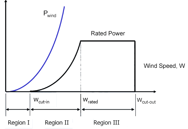
Figure 2a-1 below illustrates a typical power curve of a modern, pitch-controlled, horizontal-axis wind turbine. It is plotted as power versus wind speed. The solid blue line (Pwind) denotes the power available in the wind. Wind power is proportional to the cube of the wind speed, as shown by the Pwind line. What does this mean? If you double the wind speed, the result is an eight fold increase in the power you can capture from the wind.
The following video explains the 3 wind (or power) regions from Fig. 2a-1:
Transcript: Power Curve of Pitch-Controlled HAWTs
A real wind turbine, if you look at it, it's going to take a bit of a wind speed to start it. So there is a region from zero wind up to a certain wind speed, called the cut-in wind speed, where there is no power produced by the wind turbine. Also called the region 1. Nothing is happening. Then, once the cut-in wind speed is reached, power ramps up and you see that it's in an almost parallel slope to the power that becomes available with the wind speed itself. But it's only a certain fraction of that amount that actually a machine, a wind turbine rotor, can capture. We're going to learn about how much that is. That region is called region 2. Power ramps up.
Ideally, you want to produce power with wind turbine and you want to make money. Right, you want to sell the power. Ideally you want to go all the way up here, but you're limited. What limits you? Generator. The first thing that limits you is the generator. Generator can only take so much power, and feed it into the electrical grid. You have to start controlling the power. That's the typical power curve of a modern pitch controlled horizontal axis wind turbine. You control the power by changing the blade pitch. Changing the load and hence the torque and power produced by the rotor. That wind speed where you reach the rated power of a turbine and the generator is called the rated wind speed. From there on as the wind speed increases, we're going to see you have to pitch more and more the blades to accommodate for the fact that more wind power is coming in, but you can only allow to capture so much of that. Essentially you have to adjust the blade pitch angle such that local angles of attack acting on local airfoil sections become smaller, and hence the loads the become relatively smaller and the power stays the same.
So then back at the end here, usually if the wind speed becomes about 25 meters you have to shut down the turbine. Why is that? It's not a generator problem. It's the blade loads. Becomes a load and fatigue issue. Storm condition also. In a storm, you have more fluctuations, large amplitude and that poses a problem, you have to shut down the rotor. That's the cut-out wind speed. So we have these 3 distinct regions, in a power curve of a modern pitch controlled horizontal axis wind turbine.
Actuator Disk Model
The flow field around a wind turbine rotor is very complex. The blades of today’s utility-scale wind turbines are equipped with various airfoils that are optimized to perform at their respective position along the blade span. Depending on the wind speed, blades are pitched collectively to either maximize the power extraction at a given wind speed or to control the power production for wind speeds larger than rated. Furthermore, the blades experience elastic deformations and are exposed to wind gusts, turbulent eddies, and an incoming sheared wind profile of the surrounding Atmospheric Boundary Layer (ABL).
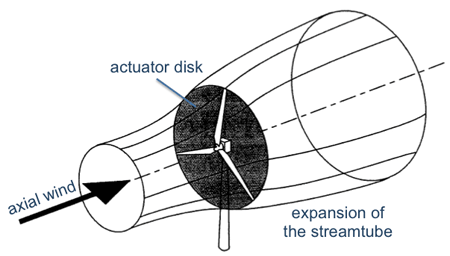
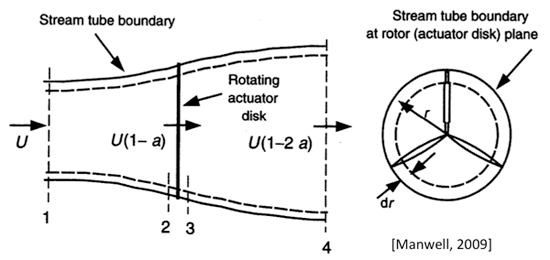
The apparent problem complexity includes time-varying, three-dimensional, turbulent flow with vortical structures. It seems impractical to gain some basic understanding in power production and blade loads without significantly simplifying the problem. For this purpose, let us think about the wind turbine as a device that extracts momentum and energy from the wind, and does so ‘uniformly’ over the rotor swept area (as indicated in Fig. 2a-2). We can hence consider the rotor as an infinitesimally thick actuator disk (surface) that reduces the momentum of the axial wind.
A one-dimensional and axi-symmetric model in fluid dynamics is that of the streamtube, see again Fig. 2a-2. As the wind turbine extracts momentum and energy from the axial free stream, the wind inside the streamtube slows down. Consequently, the streamtube has to expand in order to satisfy mass conservation in the former.
We add a further assumption to the problem that concerns neglecting shear effects within the streamtube. This means, in particular, that there is a uniform wind profile entering and exiting the streamtube. Hence, viscous losses are neglected (inviscid) that prohibit the generation of vorticity and associated vortical structures such as root- and tip vortices (irrotational). We further assume that the actuator disk be stationary (no rotation) and that the uniform wind entering the streamtube does not change in time (steady).
Let us summarize the assumptions the Actuator Disk Model: steady, 1-D, inviscid, irrotational, no rotation.
Basic Streamtube Analysis
Let us refer to Fig. 2a-3 (top plot) for a cross-sectional view through the streamtube. We can see that a uniform wind profile V0 enters the streamtube. The wind speed inside the streamtube continuously decreases (lower plot) as the wind turbine extracts momentum and energy from the wind profile that enters the streamtube. At the actuator disk, the uniform wind profile is of magnitude u; at the exit plane of the streamtube, the velocity magnitude has reduced to u1. We note that the wind speed V0 outside the streamtube remains unchanged.
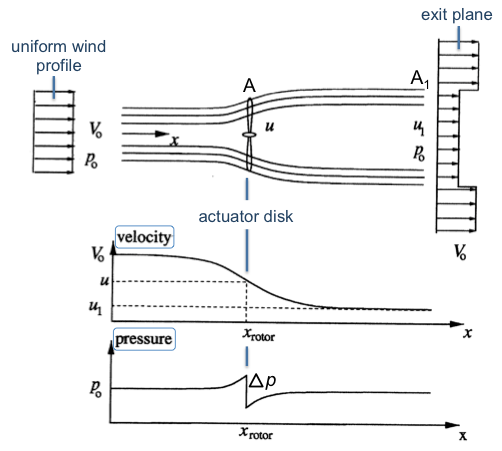
Before proceeding, let us have a closer look at the exit plane where two uniform velocity profiles come together. An abrupt velocity gradient is present, however our assumption of inviscid and hence irrotational flow allows for ‘free’ slip along the streamtube. Therefore, no friction losses are present in the analysis. – While the velocity distribution along the streamtube is continuous, the situation is different for the static pressure. It is obvious that the local static pressure has to equal the ambient pressure p0 at the streamtube entrance and exit. However, the continuous flow deceleration inside the streamtube demands an increase in pressure according to Bernoulli’s law (which we will refer to a little later). Therefore, the only way to satisfy that the static pressure at streamtube entrance and exit equals p0 (ambient pressure) is to have a pressure discontinuity Δp at the actuator disk. It is this pressure jump that acts as an external force to the fluid and extracts the axial momentum, respectively energy and power.
In the following, let us write down some familiar engineering relations.
We can write the Rotor Disk Area as a function of rotor diameter D as:
As for the Mass Flow Rate (m*) through the streamtube, we can evaluate it at the actuator disk:
and at the exit plane (noting that the exit area A1 at the streamtube is thus far unknown to us):
The pressure jump Δp across the actuator disk acts on the rotor disk area A to produce the thrust force T of the wind turbine:
We note that the thrust force acts downwind in the streamwise direction. This is a consequence of the fact that a wind turbine extracts axial momentum and energy, which is opposite to the behavior of a propeller that generates an upwind thrust force by accelerating the fluid at the expense of engine power. From Newton’s second law, we know that a force equals a change in momentum. Considering the streamtube as a control volume we find that the thrust force T is the only external force acting on the control volume and that this force is balanced by the momentum fluxes that enter and leave the control volume:
As for the power P (which is what we really want in Wind Energy), we remember that power equals energy per unit time. The wind turbine extracts ‘kinetic’ energy from the wind, hence the amount of power being extracted equals the difference in kinetic energy fluxes entering and exiting the streamtube control volume:
In order to compute rotor thrust T and power P we need to find the velocities u and u1 at the actuator disk and at the exit plane. In addition to mass conservation and Newton’s 2nd law we can apply the classical incompressible Bernoulli equation to the flow inside the streamtube. We note, however, from Figure 2.2 that the pressure is discontinuous across the actuator disk. Hence the Bernoulli equation can only be applied upstream and downstream of the pressure discontinuity.
Video Question: What are the conditions in order to apply Bernouli's Equation?
Transcript: Conditions for using Bernoulli's Equation
When can you use Bernoulli's Equation? Steady, Inviscid, irrotational, incompressible, and there's a fifth one. Anybody remember the fifth condition? That's the one that is not going to make it work here. Conservative body forces. What is an example of a conservative body force? Gravity is a conservative body force. How about pressure jump? Is that conservative? No, it's not. It's like a shock wave. That means you can NOT apply Bernoulli's Equation all across here, but break-up the problem and apply Bernoulli's Equation upstream of the actuator disk and downstream of the actuator disk. That's exactly what we are going to do next.
Bernoulli Equation
We begin by writing the Bernoulli equation ‘upstream’ of the actuator disk as:
In this equation, p is the pressure slightly upstream of the rotor disk. If we define the pressure drop across the actuator disk as Δp, then the pressure just downstream of the actuator disk becomes p-Δp. We can then write the ‘downstream’ Bernoulli equation as:
Subtracting the upstream and downstream Bernoulli equations from one another relates the pressure drop Δp to the unknown velocities u and u1:
We can use the relation for the pressure drop Δp in the equation for the thrust:
...to obtain u:
It is interesting to observe that the velocity u at the actuator disk is the arithmetic average of the velocities entering and exiting the streamtube.
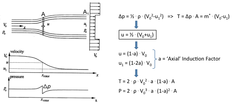
It is practical in many engineering problems to use dimensionless coefficients (figure 2a-4). Let us define an ‘axial induction factor a through u=(1-a)⋅V0 which describes the velocity u at the actuator disk as a fraction of the free stream wind speed V0.
Using u=½⋅(V0+u1) we can write the velocity u1 at the exit plane as u1=(1-2a)⋅V0. It becomes evident that in the special case of a=0, the unknown velocities u and u1 simply equal the free stream wind speed V0 and both thrust T and power P are zero.
A couple things about thrust and power:
Transcript: Thrust and Power
We note a couple of very important things. Number one is thrust is proportional to the square of the wind speed. And that is also reflected in a quadratic dependence on the axial induction factor a. While the the power P is proportional the cube of the wind speed. We had mentioned it earlier. And that is also reflected in a third order dependence on the axial induction factor a.
2a.2 The Actuator Disk Model
Rotor Thrust and Power
Next, we use the derived equations for u and u1 in those for the thrust T and power P and obtain:
We hence obtained thrust T and power P as a function of air density ρ, wind speed V0, actuator disk area A, and the ‘axial induction factor’ a. It is convenient to write both physical quantities in an appropriate dimensionless form.
As for the thrust T, we use the dynamic pressure acting on the actuator disk as the normalization factor:
For the power P, we use the available ‘power in the wind’ Pavail passing through the rotor disk area A as the normalization factor:
We can thus define a thrust coefficient CT and power coefficient CP as:
Both are dimensionless quantities and are sole functions of the axial induction factor a.
This means in particular that thrust T and power P can be written as:
The previous equation illustrates the key dependencies for thrust and power:
- The thrust T is proportional to the wind speed squared, the rotor diameter squared, and the thrust coefficient.
In general, one aims at minimizing the rotor thrust for a given wind speed and rotor diameter, i.e. as small values of CT as possible are desired.
- The power P is proportional to the wind speed cubed, the rotor diameter squared, and the power coefficient.
It is obvious that one would aim at maximizing the power coefficient CP given a wind speed and rotor diameter. However, we note that there is just a linear proportionality of rotor power to the power coefficient. The biggest effect on the total power P is due to the wind resource V03 and rotor size D2.
Let us consider again the relations for the thrust coefficient CT and power coefficient CP as sole functions of the axial induction factor a.
We note that CT is a quadratic function in a, while CP is a cubic function in a. Next, we plot the dimensionless quantities CT and CP versus their dependent a in order to find some basic limitations on rotor thrust and power.
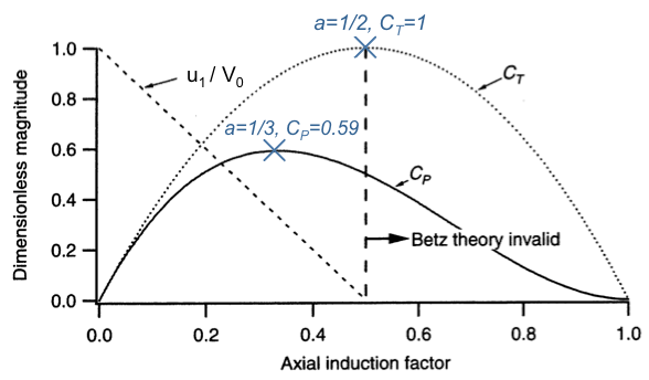
As for the thrust coefficient CT, we find it to be of parabolic shape symmetric about a=0.5. Its maximum value is CT=1, which makes the rotor thrust being equal to the dynamic pressure force on a solid actuator disk. (Figure 2a-5.) See definition of CT in equation (2.16).
Transcript: Thrust Coefficient and Power Coefficient
Let's plot some of the results that we have learned. We want to plot the dimensionless magnitudes of the the thrust coefficient CT and the power coefficient CP verses the axial induction factor a. But first let us remember what these relations were. The thrust coefficient C sub T, we had 4a(1-a). And for the power coefficient C sub P, we found it to be 4a(1-a) squared. In other words, thrust coefficient exhibits quadratic dependence on the axial induction factor a, while the power coefficient shows a cubic dependence.
Let's start first with the thrust coefficient CT. The quadratic demands that it is a parabola. So if a is zero, naturally that becomes zero. Also the thrust coefficient is zero for a being equal to 1. The dotted line here represents the parabola. You can show easily that this parabola will have a maximum for an axial induction factor a=1/2, in which case the maximum thrust coefficient becomes one.
Things are a little different for the power coefficient CP because we have this cubic dependence. But again, if a is zero, the power coefficient is zero and also for a=1, the power coefficient will be become zero. There a are few subtleties to the power coefficient, that is the cubic dependence give us the maximum, the minimum and the inflection point somewhere in between. We will derive, later, that the maximum power coefficient of CP=0.59 is obtained for an axial induction factor a=1/3.
Now just remember that power is something that's good for us, we want to capture as much power as we can. Thrust, well, if we can reduce it to a minimum better, because the thrust force of the rotor is creating a large bending moment to the tower and foundation of a wind turbine.
One more thing I'd like to point out here is that we need to be aware of the exit velocity u sub 1 out of the streamtube. Why is that? We found earlier that u1/V knot is a fuction of A2 and that equals 1-2a. Now, if a, the axial induction factor, becomes larger than 1/2, something happens and that is u1/V knot, the wind speed, becomes less than zero. In other words, the exit velocity out of the stream tube is reversed. If the flow reverses, also called the turbulent wake state, that is something that is absolutely not compliant with the assumptions that we put into momentum theory. And this is why here is the diagram, it's indicated for a>1/2 the Betz theory or momentum theory becomes invalid. The maximum power coefficient, we shall see later, is also called the Betz limit.
So far so good, let's move on to the next subject.
Find CT,Max:
As for the power coefficient CP, we find that its maximum value is approximately 0.59 for an axial induction factor of a=1/3. (Figure 2a-5.)
Find CP,Max:
With reference to the definition of the power coefficient CP in equation (2a.17), it becomes clear that we can at the most harvest approximately 59% of all the kinetic energy in the wind that passes through the streamtube.
The upper limit for the power coefficient CP,max=0.59 is called the “Betz Limit”.
Figure 2a-5 also illustrates a diagonal dashed line representing the ratio of the streamtube exit velocity u1 and the wind speed V0. From Figure 2a-4, we can see that u1/V0 depends linearly on the axial induction factor a. It is not surprising that u1/V0=1 for a=0, as in this case of zero induction both rotor thrust and power equal zero. However, the ratio u1/V0 becomes negative for a>0.5. This means in particular that there is reverse flow at the exit of the streamtube. This flow state is called the “turbulent wake state” and violates the assumptions of inviscid and irrotational flow of the actuator disk model. We thus conclude that the actuator disk model is valid for axial induction factors a<0.5.
Wake Expansion and Wake Shear
Figure 2a-6 shows that as the thrust coefficient CT increases, i.e. increasing axial induction factor a, the streamtube expands with decreasing entrance area A0 and increasing exit area A1. Note that there is always the wind speed V0 entering the streamtube, while we saw that the exit velocity u1 is a linear function of the axial induction factor a. As a consequence, there is a discontinuity between the exit velocity u1 and the ambient wind speed V0.
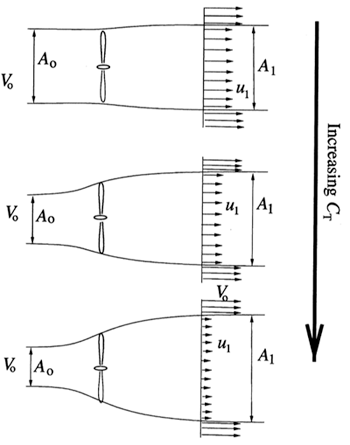
Now remember that the streamtube is a fictitious surface that allowed us to apply mass, momentum, and energy balances within the assumptions of the actuator disk model. In reality, the discontinuity between the streamwise velocities inside and outside the streamtube generates a ‘viscous shear layer’ in the wake. It has been found that wake shear becomes very strong for u1/V0<0.2 or a>0.4. This further limits the validity of the actuator disk model to axial induction factors a<0.4.
Wake Expansion
- Velocity Jump u1/V0
- Rotor Thrust CT
Wake Shear
- Dominant for u1/V0 < 0.2
- Turbulent eddies
Validity of Momentum Theory
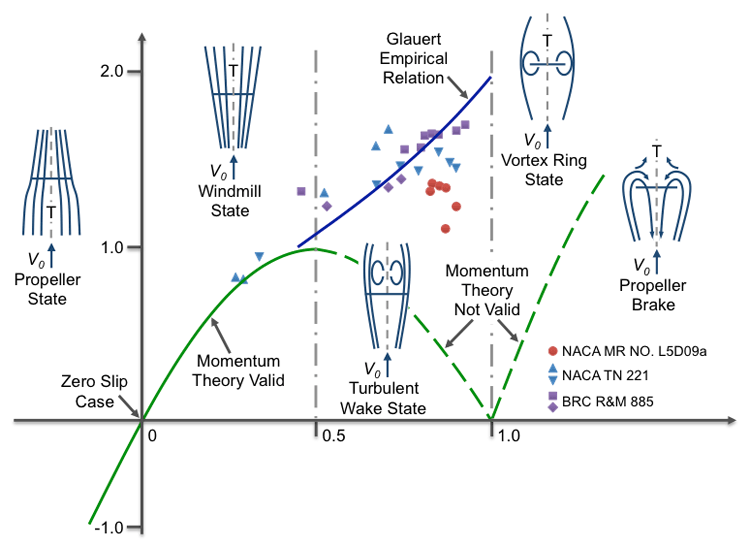
Figure 2a-7 below presents another illustration concerning the validity of the actuator disk (or momentum) theory. Plotted is again the thrust coefficient CT versus the axial induction factor a. For a<0, we are in the propeller state where the streamtube is contracting, and the thrust force is directed upstream and acts as a propulsion device. Note that one has to provide energy to the fluid for a<0. For 0<a<0.4, we are in the windmill state where momentum theory is indeed valid. The streamtube is expanding, and the thrust force is directed downstream and acts as a drag force. In this case, we are extracting energy from the main flow stream.
The second half of the CT parabola (a>0.5) is plotted as a dashed line with an indicator that momentum theory is invalid. This is the ‘turbulent wake state’ that begins with a=0.5 and reverse flow at the exit plane that progresses towards the actuator disk with increasing axial induction factor a. For a=1.0, the reverse flow has reached the actuator disk, and the rotor enters the ‘vortex ring state’. This special flow state can be very dangerous for helicopter rotors. At approximately a=0.4, a solid line ‘Glauert Empirical Relation’ connects the CT curve for momentum theory to the limiting value of CT=2.0 that represents the drag coefficient of a flat plate at 90 degrees angle-of-attack.
The symbols denote experimental data obtained by Glauert in the 1930s. The steep increase of the thrust coefficient CT for a>0.4 is attributed to flow separation and stall. In general, one would aim at operating a wind turbine rotor between 0<a<0.4 as close as possible to the CP,max at a=1/3.
Transcript: Momentum Theory
Wow, there's a lot of information on this diagram, so let's put some order in this. What we're actually showing here is the thrust coefficient on the vertical axis, again plotted verses the axial induction factor a. So here we have the thrust coefficient and here we have the axial induction factor a. And we're doing that for all kinds of rotary wings, aerodynamic flow states.
What we know so far is, well, we know the parabola, we recognize the parabola for the thrust coefficient, which is the green line here. And yes, the green line turns from solid into a dashed line for axial induction factors a>1/2 because we saw that in this case the exit velocity at the end of the streamtube reverses and because of that, momentum theory is no longer valid. What happens now is actually at some point this reverse flow is reaching the rotor disk area itself. It moves progressively towards the rotor disk area as the axial induction factor a increase. Ultimately, if the reverse flow region hits the rotor disk area, we enter the so-called vortex ring state. That's something that's very dangerous if you're flying in a helicopter, and the only was a helicopter pilot can get out of this situation is by moving the helicopter to the side or moving forward. If the axial induction factor is yet further increased, the vortex ring states turns into the propeller brake state. Everything here is highly non- linear and absolutely not something momentum theory can help us with.
So what do we do if we get into the turbulent wake state? What happens here? Well, there is a number of experiments, you see these symbols here that were conducted a NACA and BRC, and for propellers of different solidity and advanced ratios or tip speed ratios you name it, it's kind of a shot gun approach. And what the solid blue line is showing here is sort of a curve fit, and we know the curve fit has to be tangent at some point to the solid green line, the momentum theory is valid. And in the end, for an axial induction factor of a=1, the thrust coefficient becomes 2, which is related to a flat plate drag coefficient. Later on in the course, when we talk about blade element solution algorithm, this empirical relation that attributed to Glauert, will be further explained and be worked with.
Wait a minute, what happens actually if the axial induction factor is zero and become negative? Well we saw the reason why the wind turbine takes energy is because it slows down the main flow. Meaning, the velocity at the rotor disk itself is equal to V knot, the wind speed, times 1-a. So it reduces it. So now if a become negative, 1-a become positive, so we're actually accelerating the flow at the rotor disk. In that case, the windmill becomes a propeller. And still in propeller theory, we also have a region where momentum theory is indeed valid.
One more thing I'd like to point out here, in the wind mill state, the steamtube is expanding, we know that, and the thrust is directed in the flow direction. So it's really a drag, not a thrust. This changes in the propeller state. The propeller accelerates the flow thus the streamtube contracts and the propeller generates a jet in its wake and the result of that is that the thrust force is in opposite direction towards the incoming air speed and the thrust is really a thrust. The propeller is propelling us forward, while the wind turbine in that case, the thrust is more of a drag and it's pulling the rotor backwards and generating a large bending moment on the tower and foundation.
Actuator Disk Model Summary
Let us summarize once more the assumptions and main results of the actuator disk model :
- 1-D, Inviscid, Irrotational, NO Rotation, Steady
- Includes effect of tip speed ratio λ = (Ω · R) / V0
- Rotor Power: P = P(V03, D2, CP)
- Wind Turbine Power Production driven by …
- Wind Resource, V0
- Rotor Size, D
- Blade/Rotor Design, CP & CT
- “Betz Limit” CP,max ≈ 0.59
- We can only capture a Max. of 59% of the energy in the wind!
2a.3 The Rotor Disk Model
Introduction
Our next step is to develop “The Rotor Disk Model” that allows for rotation of the actuator disk and the downstream wake. The following assumptions, though, remain:
- One-Dimensional
- Inviscid & Irrotational
- Steady
In the simplified model of a rotor disk, we still consider a streamtube, however we proceed one step towards an actual wind turbine rotor by adding a ‘swirl’ or ‘rotation’ to the wake. Without further analysis, we surmise that the addition of wake rotation to the flow inside the streamtube is associated with a loss in power produced by the rotor disk as additional kinetic energy is needed to sustain the rotation of the wake.
The actuator disk theory revealed that the maximum power coefficient CP is governed by the Betz limit of CP,max=0.59. We will find that adding wake rotation will decrease the theoretical maximum. – The actuator disk theory generated the rotor power via the rotor thrust and the axial induction factor a. In rotor disk theory, on the contrary, we will discover that rotor power is generated through rotor torque and the angular momentum in the wake via a combination of axial- and angular induction factors.
Transcript: Actuator Disk to Rotor Disk - Introduction of Wake Rotation
The Betz limit is the limit, 59% of the energy that we can capture from the wind. Now, if you allow the actuator disk to become a rotor disk that's spinning at some rotor speed omega, the side of effect of doing that is that you add a swirl to the downstream wind. Adding a swirl means you have to pay for it. You have to pay for it with momentum and energy. In other words, that side of effect of the method that makes you adding that swirl, is that you cannot capture as much energy as in the actuator disk model. So we will get something that is less than the Betz limit for sure. The question is how much is that.
Rotor Torque and Power
At first, let us recall from classical mechanics that rotor torque is associated with a change in wake angular momentum:
Rotor Torque = Change in Wake Angular Momentum
We denote the rotor speed or the angular velocity of the rotor disk by Ω (Omega). The wake speed, respectively, is the sum of the rotor speed Ω and the swirl speed ω (omega). We thus have:
Rotor Speed: Ω
Wake Speed: Ω + ω
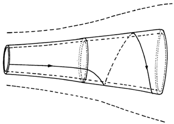
Next, we consider an annulus of width dr of the rotor disk and write the incremental torque dQ acting on the annulus as...
...where the term in brackets represents a mass moment of inertia flowing through the considered annulus of the rotor disk.
Transcript: Mass moment of inertia
The mass moment of inertial, you have to be careful. I cannot just take the entire disk to do it. Because the mass moment of inertia is something that changes with distance over mass to the center of rotation. So I take the ring or annulus out of that rotor disk and consider what will be the incremental torque distribution of that.
We make use of the definition of the mass flow rate in eqn. (2a.2) dm* = ρ · u · dA and write the incremental torque as:
We also remember from previous analysis that the velocity at the rotor disk is u = (1-a)·V0 , and note that an incremental area dA of a rotor disk annulus is dA = 2 πr · dr
We can also define an incremental power and an incremental power coefficient in the following way:
Rotor Torque and Power
Our next task is to find an expression for the incremental power coefficient d CP. Before proceeding, though, let us define some additional dimensionless parameters that will he helpful in the analysis and useful to a thorough understanding of the effects of wake rotation.
Angular Induction Factor: a' = ω / (2 Ω)
Tip Speed Ratio: λ = (Ω · R) / V0
Local Tip Speed Ratio: λr = λ · r/R
The ‘angular’ induction factor a’ is defined as being proportional to ω. It is apparent that in the special case of ω = 0 the angular induction factor becomes zero, and the rotor disk model reduces to the original actuator disk model. The next parameter, i.e. Tip Speed Ratio λ, involves the rotor speed Ω and describes the ratio of the blade tip speed Ω · R to the wind speed V0. We will see later in this course that typical values for λ range between 4 and 7. The third parameter shown is the Local Tip Speed Ratio λr, which is simply a fraction of λ based on the local blade position r/R.
Using these newly defined parameters and performing some algebra on the incremental power dP we obtain
...which gives us the incremental power dP as a function of wind speed V0, blade radius R, the rotational parameters λ and λr, and the dimensionless axial- and angular induction factors a and a’.
Hence, the differential power coefficient dCP becomes
Transcript: differential power coefficient dCp
The incremental power coefficient of an annulus on the rotor disk is a function of the tip speed ratio, the angular induction factor, the axial induction factor, and the local tip speed ratio, which is simply a product of the actual tip speed ratio times you local relative location along the blade.
The power coefficient CP of the wind turbine is obtained by integrating the previous equation along the entire rotor disk, specifically for λr ranging between 0 and the tip speed ratio λ.
As the integral for the power coefficient CP is performed over the local tip speed ratio λr, our next task is to find two relations between λr and the axial- and angular induction factors a and a’, which will enable us to compute the integral in (2a.27). We will do so by considering the following:
First, let us remember equation (2a.9) from actuator disk theory that related the pressure jump Δpa across the actuator disk to the axial induction factor a.
Actuator Disk: Δpa = ½ ρ (V02 - u12) = 2 ρ V02 a (1 - a)
What approach would we take for the Rotor Disk?
Our approach consists of having the same pressure jump cause the wake rotation ω. Hence, we are looking for Δpa’ = Δpa. In actuator disk theory, we used the Bernoulli equation applied to the axial velocity component through the streamtube.
We will use a similar approach here, however considering only the angular (or rotational) velocity. We write the Bernoulli equation as:
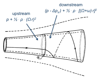
And substitute ω using the definition of the angular induction factor, i.e. a’ = ω / (2 Ω). Thus, we find for the pressure jump Δpa’:
Equating both formulations for the pressure drop across the rotor disk, i.e. Δpa = Δpa’ , we obtain the following after some algebra:
Transcript: First relationship between a and a'
And this omega times r/V0 square is again the square of the local tip speed ratio lambda r. So we isolate this on the right hand side and so on the left hand side you get the ratio of a(1-a) divided by a'(1+a').
The above equation constitutes a first relation between a, a’, and λr . In order to evaluate the integral for the power coefficient CP in (2a.27), we must find a second relation.
We mentioned earlier that the addition of wake rotation is likely to reduce the maximum power coefficient CP,max=0.59 due to Betz in actuator disk theory. One of our objectives in rotor disk theory is to understand to what extent do the newly introduced parameters a’, λ, and λr reduce the Betz limit. By inspecting the integrand in (2a.27) we realize that the maximum power coefficient occurs for the integrand factor a’(1-a) attaining a maximum for each λr. We therefore want to maximize the function f(a, a’) = a’(1-a). As a first step, let us compute the first and second derivatives of f(a,a’) using the product rule:
Next, we must perform the necessary algebra find the second relation between a and a'.
2a.4 The Rotor Disk Model
We've just shown that the 2nd relationship between a and a' may be an extreme, but we don't know yet if this relation will result in maximized or minimized power. In order to better understand this, we have to look at the second derivative of d2f / da2.
Check the second derivative...
...from the first derivative...
...and the first derivative of eqn. (2a.30) ...
Remember the first equation (2a.30) equated the pressure differences. We now also have its first derivative, and we will take its second derivative as well and obtain:
Now we use all of the above relations in the second deriviative:
Assuming that the 1st derivative is equal to 0, we know that:
Thus, we can indeed find that …
Transcript: Maximum
If this is larger than zero, this last term here is less than zero. Agreed? 2(1-a) has a minus here. 2 is larger than zero. 1-a larger than zero. Lambda r square larger than zero. That's 1+squared larger than zero. Larger, larger, (1-2a), a is small enough, larger than zero. da'/da, I just looked at it. Larger than zero. So that's all larger than zero. There's the minus sign that makes it smaller than zero. This is all smaller than zero. So we can say at this point, indeed, the second derivative df by da square is less than zero. With the first derivative being equal to zero, second derivative less than zero, it means that we were really looking for a maximum in the power coefficient. That's all we wanted. That's probably one of the, most painful things that we're going to in the whole class, but it's in no text book. That's why I like to do that with you. So you know exactly where it comes from. Won't be everything like this. I promise.
So far we have eqns. (2a.30) and (2a.32), for a and a'. Equation (2a.30) was a result of equating the pressure drop across the disk:
And equation (2a.32) from maximizing the integral for the pressure coefficient:
Now we have 2 equations and 2 unknowns. We can take a' from eqn. (2a.32), which is a sole function of a and plug it into eqn. (2a.30) to find an explicit relation for a.
That gives us now the axial inductor induction factor a as a function of λr , which is scaled tip speed ratio, along the blade for maximum power.
Now, what is the actual CP,Max?
We take the derivitive d/da of boxed equation (2a.42) above and obtain:
Now take eqns. (2a.32), (2a.42), and (2a.44) in the relation for CP,max, and we get the following:
At the root where λr = 0, this will define the lower bound of the integral of CP,max with respect to a.
For the upper bound at the tip where λr becomes equal to the actual tip speed ratio λ, it defines the upper bound for a.
Transcript: Upper and Lower Bounds
If lambda r is zero, how does the right hand side become zero? There are two options. One of the factors has to zero, right? a=1 doesn't work for us. a=1/4 yes that's the one that's going to make it zero. That defines here now the lower bound of the integral. So a1=1/4 or 0.25 For the upper bound at the tip, where lambda r becomes equal to the actual tip speed ratio, lambda, it defines the upper bound for a and that is what? So this becomes lambda square. I can look again at equation 3. And that's not an easy equation to solve for a. So we'll do that numerically.
In the table that you see here, given different lambdas, it solves equation 3 for the appropriate upper integration bound, which is a2, and then gives you the power coefficient that is associated with it. So we can look at this table and say, depending on the tip speed ration -the tip speed ratio was tip speed divided by incoming wind speed- what's the maximum power coefficient that you get? Out of all this messy analysis. Betz limit is 0.593 something, 16/27 is the exact answer. So you can see here clearly as you go up in tip speed ratio, you're getting fairly close to the Betz limit. In other words, the quicker the rotor spins, the closer you get to the Betz limit.
Think about me being a 2-bladed rotor. And I rotate very slowly, no tip speed ratio. There's a lot of mass flow passing through the rotor disk area that the blades do not work on. It's not surprising that if the tip speed ratio is small, you do not get much power. In fact, in the limit, I'm standing still, there's no torque being produced. There's no wake change in angle of momentum associated with that. But as I move quicker and quicker in rotor speed, in a given time, the blades they work on more mass flow that passes through the rotor disk area. As a consequence the power coefficient is going to go up. What is important here is to note that you get fairly close to the Betz limit with a tip speed ratio of 10 and not 1000. That's important.
The table below provides different values for the tip speed ratio, λ, and solves eqn. (2a.42) for the appropriate upper integration bound, a2. It then provides the associated maximum power coefficient. Note that the quicker the rotor spins (λ increases), the closer it gets to the Betz limit.
| λ | a2 | CP,max |
|---|---|---|
| 0.5 | 0.2983 | 0.289 |
| 1.0 | 0.3170 | 0.416 |
| 1.5 | 0.3245 | 0.477 |
| 2.0 | 0.3279 | 0.511 |
| 2.5 | 0.3297 | 0.533 |
| 5.0 | 0.3324 | 0.570 |
| 7.5 | 0.3329 | 0.581 |
| 10.0 | 0.3330 | 0.585 |
Let us get back to the integral for Cp,max:
If we use the transformation x = 1- 3a and its derivative dx/da = -3 we obtain:
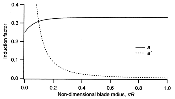
If we use this to look at the distribution, we find the induction factors a and a' as functions of the local tip speed ratio, λr, for maximum power for an example reference case of a tip speed ratio that equals 7.5.
Let us recall these numbers...
The axial induction factor where u is the axial velocity of the actuator or rotor disk, and V0 is the wind speed.
where Ω is the rotor speed.
And for the optimum case
The graph below (Fig. 2a-10) illustrates this distribution. Keep in mind that this is for a specific tip speed ratio that is fairly high at 7.5. The graph shows a and a' versus the radial position along the blade (multipy this number by the tip speed ratio 7.5. to get λr.)
The solid line represents the axial induction factor a. At the root where r or λr equals zero, the induction factor a is 0.25, and it approaches the ideal value of 1/3 towards the tip.
The dotted line represents the angular induction factor a'. In the relationship , a approaches 1/3 when a' goes to zero. Out at the tip the effect or the loss due to rotation becomes zero, and a approaches indeed the Betz limit. However, when a becomes close to 1/4, as it does at the root, we're dividing by zero and a' actually has a singularity.
Video question: In Fig. 2a-10, why does a' have a singularity?
Transcript: a' singularity
Now if you fix the tip speed ratio, the highest rotation and where you work most is out at the tip, but as you go inboard, the rotational speed becomes lesser and lesser. However, in rotor disk theory, you still have to add the swirl to the flow inboard. However, that swirl the local little omega, has a rather big portion of the actual velocity at a more inboard station. So you have capitol omega here and you add the swirl, little omega, but down here you have capitol omega times r/r, so the little omega that's acting there is larger to the actual rotation. Or another analogy, you just say well along the blade I'm sweeping over a range of tip speed ratios and you get the closest match to the Betz limit out at the tip and inboard it's less than that. Just because the local tip speed ratio is smaller there.
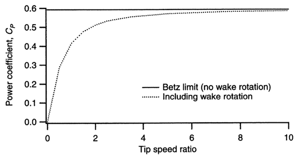
The plot below (Fig. 2a-11) illustrates the maximum power we can get including the wake rotation. We have the tip speed ratio as a free parameter λ, which equals the velocity at the tip Ω • R, divided by the wind speed V0 :
We're plotting power coefficient versus tip speed ratio. The solid line represents actuator disk theory, or the the Betz limit, which is 16/27 or approximately equal to 0.593. This is the maximum you can acheive. If your tip speed ratio is 0, the power will be zero. As you increase the tip speed ratio, the power coefficient gets closer to the Betz limit.
Video question: Is there an ideal tip speed ratio?
Transcript: Max Power
Tip speed ratio is the ratio of a tip speed to the incoming wind speed. How fast or how quick does a wind turbine have spin in order to get close to the Betz limit? Looks like from this plot, the tip speed ratio doesn't have to be 100 or 1000. This is good news. Because as you can see even for a tip speed ratio of about 5, you're already at 0.57 or so, getting pretty close to the Betz limit for a fairly low tip speed ratio. If you look at a wind turbine blade that's about 40 meters long, it weighs between 8000 and 9000 pounds. So if you double the rotor speed the centrifugal force goes with the square of the rotor speed, so that's immense. If you would have to go from 5 to 10, you're centrifugal force of this 8000 pounds that spins around gets multiplied by a factor of 4. That's significant. You don't want to do that, you want to get by with as small of a tip speed ratio as you can. Wind turbine noise is proportional between the 5th and 6th power of the tip speed. That's enormous. Any reduction in tip speed because it goes at least to the fifth power, reduces the noise significantly. And that is why for most onshore wind turbines a tip speed ratio of 4 is pretty common. Offshore in European developments in the north sea, they spin the rotors quicker. Nobody cares about the noise. But they would never go up to 10 because of structural considerations.
Validity of the Rotor Disk Model
Parameters:
The two relations between a and a':
Eliminate the λr2 by subtracting the two equations from one another and you'll find:
As we approach locally the ideal axial induction factor of a = 1/3, a' naturally goes to zero. It will also do this for high tip speed ratios. An interesting twist is that the effects of wake rotation are smallest for a quickly spinning rotor. This seems counter-intuitive at first as the loss due to wake rotation is related to the 'swirl' that's being added to the downstream flow.
In general, the higher the rotor speed, the closer one approaches the limit of the uniform-flow actuator disk. And the faster the tip speed, the smaller the relation between the ω (the swirl you're adding to the wake) and the actual rotor speed Ω.
Rotor Disk Model Summary
Let us summarize a few lines about the rotor disk model:
- 1-Dimensional, Inviscid, Irrotational, Steady
- Includes Effect of Tip Speed Ratio λ = (Ω·R) / V0
- Rotor Power still remains a function of the 3-2-1 law: P = P(V03, D2, CP(λ) )
- Approaches “Betz Limit” of CP,max ≈ 0.59 for high λ
This is the essense you should you know as well as how to sketch the relative distributions of a and a' prime versus radius and for different tip speed ratios.
XTurb-PSU Training
XTurb-PSU is design and analysis code used here at Penn State. It is maintained and developed by Dr. Schmitz and his students. Below you will find several videos to help train you to use this code for your homework assignment.
Quick links:
XTurb Screencasts
Each screencast below covers a section of the XTurb training.