Lesson 5
Overview
About Lesson 5
Astronomers are able to gather an immense amount of information about stars—their temperatures, their velocities, their distances, their chemical compositions, and also variations in these quantities. Given all of this data, we can construct a physical model for stars that accurately reproduces the observable quantities. The accuracy of our models at reproducing the properties of stars suggests that we understand the internal structure of stars quite well.
Our observations and our theory of stars show us that the stars are not eternal, unchanging objects. Stars follow a lifecycle: they are born, they change slowly as they age, and eventually they die. In this lesson, we are going to focus on the birth of stars and discuss how their lives begin. We will conclude by studying some special cases, including failed stars, bound pairs of stars, and variable stars.
What will we learn in Lesson 5?
By the end of Lesson 5, you should be able to:
- Describe the process by which stars generate energy in their cores;
- Describe the forces that keep stars in a stable equilibrium;
- Qualitatively describe the process of star formation;
- Describe the early stages of the lifecycle of all stars;
- Describe how astronomers use binary stars to determine stellar masses.
What is due for Lesson 5?
Lesson 5 will take us one week to complete.
Please refer to the Calendar in Canvas for specific time frames and due dates.
There are a number of required activities in this lesson. The chart below provides an overview of those activities that must be submitted for Lesson 5. For assignment details, refer to the lesson page noted.
| Requirement | Submitting your work |
|---|---|
| Lesson 5 Quiz | Your score on this quiz will count towards your overall quiz average. |
| Discussion: Binary Star Evolution | Participate in the Canvas Discussion Forum: "Binary Star Evolution". |
| Unit 2 lab | During lesson 5, you will begin work on the HR diagram lab listed under Lab 2, part 1. |
Questions?
If you have any questions, please post them to the General Questions and Discussion forum (not email). I will check that discussion forum daily to respond. While you are there, feel free to post your own responses if you, too, are able to help out a classmate.
The Interstellar Medium (ISM)
Additional reading from www.astronomynotes.com
- Stellar Evolution Stage 1: Giant Molecular Cloud
- Gas in the Milky Way: HII Regions
When you observe the night sky, you see the stars as pinpoints of light against a black background. You have also probably been told that outer space is a “vacuum”—that is, that, other than stars and planets, it is very empty. It is true that space is so empty that it is a more perfect vacuum than we can create in the laboratory on Earth; however, space is not completely empty. Here are some images that show some obvious examples of regions in space that contain some material between the stars:
- APOD: Orion Nebula
- APOD: Horsehead Nebula (note, the Horsehead is a small part of the Orion Nebula)
- APOD: A Giant Molecular Cloud
- APOD: The Carina Nebula Panorama from Hubble
- APOD: Reflection Nebula in M45
- Hubblesite: A Bok Globule
- Hubblesite: The Eagle Nebula
In all of these images, you see different regions of space that are either filled with what appears to be glowing gas (similar to a neon light), or dark regions that are obscuring the stars behind them. All of these objects are called nebulae, a word which is Latin for "cloud." Taken as a whole, the gas and dust that fills the space between stars is called the interstellar medium.
If you look at the images at the links above in some depth, you'll see some or all of the following:
- Clouds that glow an almost uniform, bright red;
- Dark clouds that appear to block all or most of the light of stars or bright clouds behind them;
- Clouds that glow a blue color very similar to the blue of our sky.
At this point, let's address the physical processes responsible for the appearance of these various nebulae, and give them more descriptive names.
Emission Nebulae
As the name implies, emission nebulae emit emission spectra, not continuous or absorption spectra. If you refer to the lesson on the production of emission lines, what is required for a cloud of gas to emit an emission spectrum is for electrons in the gas to be in energy levels above level 1. As they move down to the ground state, they will emit photons of specific energies, producing emission lines at those specific energies. One point we glossed over in that lesson is: How do the electrons get into the higher energy levels in the first place? In the case of emission nebulae, there is a clue usually quite apparent in the image. For example, in the image below of massive stars in NGC 6357, you see a large region of glowing red emission nebula surrounding a number of massive stars (although there is no way to tell just from looking at the picture that they are massive stars).

The massive stars give off a lot of ultraviolet light, which the hydrogen gas absorbs. The electrons in the H atoms absorb so much energy that they are actually stripped completely from the H atoms, creating a sea of hydrogen nuclei and free electrons. This is a process called ionization. The free electrons can recombine with the hydrogen nuclei, and then, as they cascade down to the ground state, they emit photons. Because the clouds are primarily made of hydrogen, the spectrum of a typical emission nebula shows strong hydrogen emission lines. The strongest hydrogen line in the visible part of the spectrum is H-alpha at 656.3 nm, which is in the red part of the spectrum.
Astronomers refer to neutral hydrogen atoms as HI (pronounced "H-one") and they refer to ionized hydrogen nuclei as HII ("H-two"). For this reason, the glowing red emission nebulae found surrounding massive stars are often referred to as "HII Regions."
We will talk about these later, but there are objects known as planetary nebulae that also give off emission spectra. Here is an example emission spectrum from a planetary nebula taken by Prof. Robin Ciardullo of Penn State:

On the x-axis is wavelength in Angstroms (1 Angstrom is 1/10 of a nanometer, so 656.3 nm = 6563 Angstroms), and on the y-axis is the relative flux (or apparent brightness). You can see that there are several very prominent emission lines—the H-α line at 6563 Angstroms, the H-β line at 4861 Angstroms, a helium line, and several oxygen lines, for example. In this nebula, the oxygen line at 5007 Angstroms is stronger than H-α, so this nebula will appear more green than red. This is seen in the central regions shown in the photo below.

Dark Nebulae
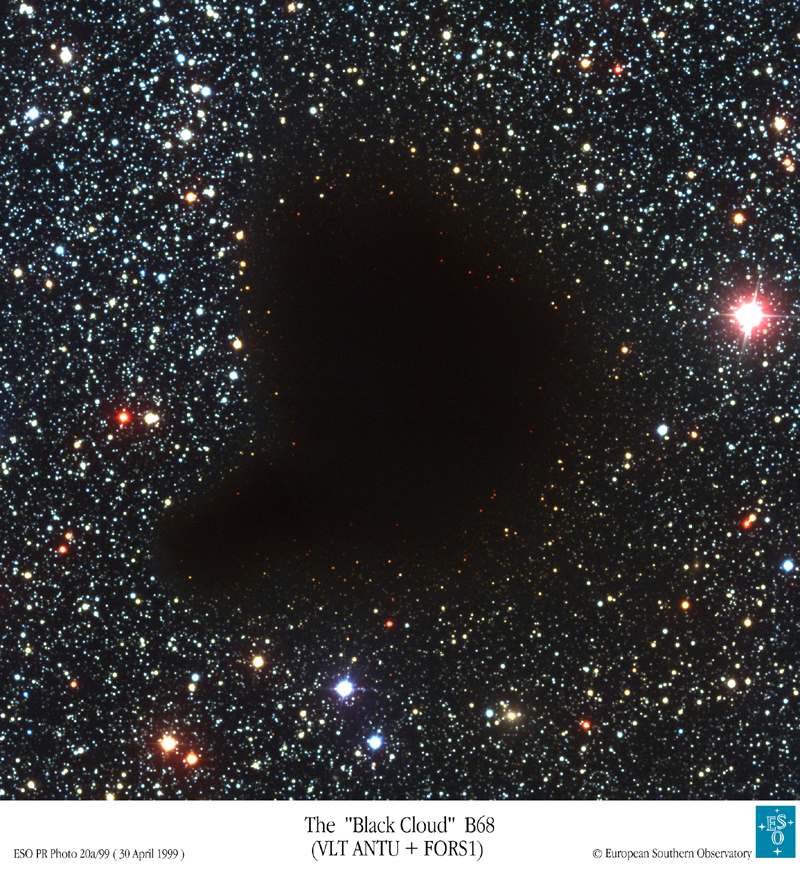
In regions where there are a lot of stars (such as in the APOD of a Giant Molecular Cloud), or regions with bright emission nebulae (such as in the Hubblesite image of a Bok Globule), we can see dark nebulae that appear to be blocking the background light sources behind them. These dark nebulae are also interstellar clouds, but unlike the emission nebulae, they are very cold (10 K, as opposed to about 10,000 K for emission nebulae) and very dense. These clouds are called molecular clouds because the conditions in them are just right for the creation of molecular hydrogen. Be aware that two hydrogen atoms that have linked together form the molecule H2 (which is also pronounced "H-two", but should not be confused with HII). Another constituent of these dark clouds is interstellar dust. The dust particles are very tiny grains of different solids, and if you compare their chemical makeup to common materials on Earth, they are similar in many ways to soot and sand. As photons of light encounter a dark cloud of gas and dust, we observe two effects: first, the light is extinguished—that is, the background light sources appear dimmer than if there was no intervening cloud. This effect is referred to as interstellar extinction. The second effect is referred to as interstellar reddening. As the name suggests, the light from a background source will appear redder than if it had not passed through the cloud. As photons of light pass through the cloud, they get scattered from their original paths. Blue light scatters more than red light, so less blue light and more red light from the background object makes it through the cloud. If you look closely at the APOD image of Barnard 68, you will see that all the stars visible near the edge of the cloud look red or orange, while those just outside the boundaries of the cloud look blue or white, which is caused by this reddening effect. Again because of the wavelength dependence of scattering by dust, most of the infrared light will actually pass through the cloud. See the image below of Barnard 68 taken through infrared filters. You can see the reddening, but you can also see right through the cloud!

Reflection Nebulae
The bright blue regions seen in some of the images above are reflection nebulae, and they are also caused by the scattering of light by dust particles. The light from a star encounters dust particles and reflects. In most cases, the particles are the correct size to scatter blue light more efficiently than red light, so the reflection nebula appears to us in the reflected blue light from the nearby star. Since the light we see is reflected starlight, the spectrum of the reflection nebula is similar to the spectrum of the star's light.
More complex nebulae
Finally, let's consider some of the images of the regions that include overlapping nebulae of different types. First, look again at the very famous picture of a region of sky called the Eagle Nebula.

The dark pillars are part of the edge of a molecular cloud. Some nearby, very bright stars (off the edge of the picture) are illuminating these pillars of gas, and their intense radiation is causing the outer layers of the molecular cloud to evaporate (this process is called photoevaporation). What astronomers have found is that this process of photoevaporation is revealing that inside the densest knots in the pillars are newly formed, baby stars. If you study carefully some of the other images, for example the panorama of Carina, you can find similar structures to the ones seen in the Eagle Nebula.
In fact, we see that all of the youngest stars in the sky live in regions with a lot of interstellar matter. It seems clear that there must be a connection between the stars and the interstellar gas. By observing these regions in many wavelengths of light, astronomers have found that new stars are formed out of the gas and dust in these clouds. The process is not completely understood, but in the following section, we will discuss how stars form.
Want to learn more?
The Eagle Nebula image is one of the most famous Hubble images ever taken, and so, PBS has made a video on the making of the Eagle Nebula image.
The Process of Star Formation
Additional reading from www.astronomynotes.com
- Stellar Evolution: The Basic Scheme
- Stellar Evolution: T Tauri and the Main Sequence
Giant molecular clouds (GMCs) are truly giant. In fact, it is difficult to choose a representative image to show you because, in most cases, you can't see the cloud (you can only see part of the cloud). For example, the famous pillars in the Eagle Nebula image are only a small part of a vast giant molecular cloud. GMCs can contain gas with a mass as much as several million times the mass of the Sun. So, you should keep in mind that a single cloud in the ISM can perhaps create thousands or millions of stars. As we discussed previously, dark clouds absorb and scatter light. As a consequence, they are quite cold, with 10 kelvin being accepted as a typical value for their average temperature. Their internal density is quite high compared to typical values for interstellar space, but still many orders of magnitude lower than the pressure in Earth's atmosphere at sea level.
Try this!
You may be familiar with the properties of gases, but, as a reminder, you can run the Colorado PhET simulation on gas properties.
- Fill the box with a light gas.
- Use the heat control to lower the temperature to 10 K, the typical temperature of a molecular cloud.
- Observe the motion of the particles in the gas.
- Use the slider on the right hand side to increase gravity.
- Again, observe the motion of the particles in the gas.
If you consider a spherical cloud of gas, you can write out the mathematical relationship for the force of gravity pulling the cloud together and the radiation pressure of the gas in the cloud resisting the inward pull of gravity. (The gas properties simulation above is an excellent demo you can use to demonstrate how gas exerts an outward pressure on the cloud.) You can then write the expression for the mass of a cloud that has these two forces exactly in balance. This quantity is usually referred to as the Jeans mass, and it can be thought of as the minimum mass for a cloud to have its internal pressure balanced by gravity. So, what happens to a cloud that exceeds the Jeans mass? The cloud will be unstable to gravitational collapse, meaning that if some event can cause the cloud to begin to collapse, its internal pressure will not be strong enough to resist the collapse. Depending on the density and temperature, clouds of thousands of solar masses in size are generally above the Jeans mass. Once the collapse begins, the cloud's density and temperature will increase.
Interstellar clouds are not very uniform, and we expect that as they collapse, they will fragment into a number of clumps. During the collapse phase of an individual clump, a few additional effects occur. First, the clump in the cloud will attract nearby gas particles, causing the clump to grow more massive. Early in the process, the cloud is still thin enough that the photons generated inside the cloud (remember, any warm gas is emitting some light) can easily escape, so that the cloud radiates light as it collapses. (It should be noted here that even though the clump is radiating light from its core, the surrounding GMC is still so dense and dusty that the light from the core does not escape, and we are not able to see these cores with telescopes that detect optical light.) At some point, though, the core of the collapsing clump becomes so dense that the radiation being generated deep inside the clump becomes trapped (it has become opaque), causing the temperature of the core to increase quickly. At this point, the core can be referred to as a protostar.
We should consider for a moment size scales. A typical interstellar cloud is of order 1014 km, or roughly 10,000 times larger than the size of the Solar System. A cloud fragment which forms one or a few protostars is of order 1012 km, or roughly 100 times larger than the size of our Solar System. By the time the core of the fragment has become a protostar, its size will be approximately 1010 km, and its temperature of order 10,000 kelvin.
The temperature in the core of the protostar is hot enough that the thermal pressure becomes strong enough to slow the collapse down to a much slower contraction. The continued contraction of the protostar converts gravitational potential energy into thermal energy, causing the object to radiate as much light as 1,000 Suns. During this same time period, conservation of angular momentum causes the initially very slowly rotating cloud to spin much more rapidly. There will be significant centripetal force to resist further gravitational collapse along the equator of the rapidly rotating protostar, but the material near the poles will not feel this same resistance. Because of this, a disk will form around the central protostar. This disk is called either a protoplanetary disk or a proplyd. We will see in later lessons that this material is perhaps the location of the origin of planets that orbit stars.
Watch this!
I have personally found it quite challenging to teach the physics behind how rotating, roughly spherical clouds of gas collapse down to form protoplanetary disks. The detail in the previous paragraph is sparse for exactly this reason; it is not easy to describe conceptually. However, the team behind "Minute Physics" has posted an excellent short video that does quite a good job at explaining how these spherical clouds collapse to form disks. I highly recommend watching their video:
- YouTube link to "Why is the Solar System Flat"
Here is an excellent image of a protoplanetary disk seen in silhouette around a protostar in the Orion star forming region:

As the contraction phase of the protostar continues, the core temperature begins to reach more than 1 million kelvin. The protostar undergoes some violent changes during this time period; the outer parts of the clump are radiating an enormous amount of light, but the amount of light varies by large amounts on short time scales. This is usually called the “T Tauri” phase, after the first such object discovered. Stars in the T Tauri phase are also sometimes observed to be emitting bipolar outflows of material. These bipolar outflows have their own name; they are usually referred to as Herbig-Haro or HH objects. Some examples can be seen at Hubblesite: HH objects.
Also, during this T Tauri / HH phase, the protostars somehow shed some of the outer layers of material leftover from the GMC, revealing them for the first time to telescopes that can detect optical light. If you recall the discussion of the Hubblesite: The Eagle Nebula image, photoevaporation is one example of a process that may strip the outer layers from the protostars in a GMC. In a molecular cloud like the one that includes the Eagle Nebula, we see that the brightest stars form first, and their intense radiation evaporates the outer layers of material hiding the smaller protostars.
Nuclear Fusion in Protostars
Additional reading from www.astronomynotes.com
- The Sun's Power Source
- Stellar Evolution: Stage 6 Core Fusion
- Stellar Nucleosynthesis
- Neutrino

By the time clumps inside of a GMC have become T Tauri “stars,” they are still not truly stars. The event that triggers the change of an object into a star is the onset of nuclear fusion in the core.
Much of the gas inside all protostars is hydrogen. Recall a few things about hydrogen from previous discussions:
- Hydrogen is the simplest atom with a single electron and a nucleus of a single proton.
- If the electrons in a gas of hydrogen atoms absorb enough energy, the electron can be removed from the atom, creating hydrogen ions (that is, free protons) and free electrons.
By the time a collapsing gas cloud has become a protostar, its core has reached a temperature of several million kelvin. At this temperature, the hydrogen in the core will be a plasma, a "soup" of hydrogen ions and electrons moving around at very high speed. Particles of like charge repel each other, so if you take two protons (both have the same positive charge) and try to push them together, the electrical force between them will provide resistance. Inside of a protostellar core, the temperature and density are high, so the protons are packed together very tightly and are moving very rapidly. When the temperature reaches a high enough point (about 10 million kelvin), the protons are moving so fast inside the core that the electrical repulsion cannot prevent them from colliding. Once they collide, they fuse together in a process that generates energy.
Inside the core of a star like the Sun, fusion proceeds via a process called the proton-proton chain. In this multi-step process, six protons fuse together and the product is a helium nucleus and two protons.
Here are the steps in equation form:
Here are the steps laid out in flow chart form:

Here are the players:
- can be referred to as hydrogen ions, hydrogen nuclei, or free protons.
- are deuterium ions or nuclei.
- are 3-helium ions or nuclei.
- are helium ions or nuclei or "alpha-particles".
- Positrons are the anti-particle equivalents of electrons, and when they encounter electrons they annihilate, creating a gamma ray photon.
The steps in the proton-proton chain are all happening at once in the core of a star, but, at a minimum, you need step one to happen twice to create two deuterium nuclei, step two to happen twice to create two 3-helium nuclei, and the result of step three is a single helium nucleus and two hydrogen nuclei. This means that the input to the process requires six hydrogen nuclei to fuse, but you get two of them back at the end, so, overall, you can summarize the proton-proton chain in this way:
This process uses up hydrogen but creates new helium, because after the reactions have finished, you have four fewer protons than you started with, but one more helium nucleus. The mass of one helium nucleus is smaller than the combined mass of four protons, so, in this process, mass has been lost. The mass that gets lost in this process has actually been converted into energy. Einstein's famous equation:
tells us that the energy (E) generated equals the mass lost (m) times the speed of light squared ( ). The speed of light squared is a big number, so even though the amount of mass lost in this process is small, the amount of energy generated is large. Since stars contain a massive amount of hydrogen, large quantities of protons are fusing in their cores every second. For example, if you calculate how much hydrogen must be converted to helium each second in order to generate the measured luminosity of the Sun, you find that approximately half of a billion tons of hydrogen is being converted into helium each second. At that rate, the Sun has enough hydrogen in its core to continue generating energy via the proton-proton chain for another 5 billion years.
The mass difference between the helium nucleus and the hydrogen nuclei is . So, the energy released is:
each time the proton-proton chain creates one helium nucleus. You can use this information to estimate the lifetime of the Sun or any other star in the following simple way:
- Calculate how much hydrogen is available to power fusion in the star's core.
- Calculate how much total energy the star can generate if it converts all of its core hydrogen into helium at the rate of per reaction.
- Calculate the lifetime of the star as the total energy it can generate by hydrogen fusion divided by the rate at which it is emitting that energy (i.e., its luminosity).
This ignores several important details, but for a typical Sun-like star, you determine that it can shine by hydrogen fusion for approximately 10 billion years.
So, now that we know how energy is generated inside a star via nuclear fusion, we can answer the following question: Why does the onset of nuclear fusion signal the transition of a protostar into a true star? The answer is that the nuclear fusion generates energy, and this energy provides enough radiation pressure to finally balance the inward pull of gravity, stopping the contraction that began when the clump of gas began to collapse in on itself. The energy generated in the star is being radiated outwards as photons of light. As the photons pass through the star, they created a net outward push (radiation pressure), which along with the thermal pressure of the material in the star, resists gravity. When the force of gravity is exactly balanced by the total pressure, we say that the star is in hydrostatic equilibrium.
There are several final points that should be mentioned on this page. The temperature that the core of a protostar reaches depends on its mass. The more massive the protostar, the hotter it gets. If the core reaches a high enough temperature (more than 20 million kelvin), a different set of fusion reactions proceed more efficiently than the proton-proton chain. This process, called the CNO (carbon-nitrogen-oxygen) cycle, occurs in stars more massive than the Sun. The CNO cycle still requires hydrogen to proceed, so even in these stars the main fuel for the fusion reaction is hydrogen. In both the proton-proton chain and the CNO cycle, one element is being converted into another via nuclear fusion. This process of creating new elements is called nucleosynthesis.
Finally, if there is no way for us to directly observe the core of a star, how do we know that nuclear fusion is indeed its power source? The answer is in the first step of the proton-proton chain—the process also generates neutrinos. Neutrinos can pass through large quantities of matter (e.g., the entire Sun) without interacting in any way, so the neutrinos that are generated leave the Sun and travel through space. They are very difficult to detect, but on Earth, several experiments have detected solar neutrinos, verifying the Sun's core is generating energy via the proton-proton chain. In 2002, the Nobel Prize in physics was awarded to Raymond Davis for the detection of neutrinos from the Sun.
Want to learn more?
Check out Raymond Davis's biography, complete with photos of his experiments!
Stellar Evolutionary Tracks in the HR Diagram
Additional reading from www.astronomynotes.com
- Types of stars and the HR diagram
- Stellar Evolution: Mass Dependence
We are now going to transition from the discussion of how stars form into studying how they evolve. The HR diagrams that we studied in Lesson 4 are very useful tools for studying stellar evolution. A typical HR Diagram (e.g., the one for the stars in the cluster M55, below) plots a single point per star to represent that star's color and luminosity (or brightness) as it is observed today. So, you can consider an HR Diagram of that type to represent a snapshot of a moment in the lifetimes of the stars plotted. At that instant, they have that color and that luminosity.

However, you can also plot a “track” on an HR diagram that represents how the temperature and luminosity of a star changes over time. For example, let's take a Sun-like (G type) star and follow it from formation until it reaches an age of about 5 billion years old (the current age of the Sun). During the early stages of the collapse of a clump inside a GMC, the object is enshrouded by gas and dust and is not visible outside of the cloud. When the object has collapsed to the point that it is considered a protostar and has an internal temperature of about 1 million kelvin, it will be radiating approximately 1,000 times the Sun's current luminosity! However, the outer layers of this protostar are cooler than the Sun, so the point we plot on the HR diagram for this protostar is above and to the right of the Sun's current location in the diagram (temperature about 3,500 K). As the protostar continues to contract, its outer layers will heat up, but its luminosity will decrease. So, the point we plot for the protostar will move down and to the left (10 Solar luminosities, 4,000 K) as it evolves. During the T Tauri phase of pre-stellar evolution, the protostar will actually fluctuate in brightness; however, on average, T Tauri stars are cooler and fainter than their final location in the HR diagram (0.7 Solar luminosities, 4,500 K). Finally, when the star is fusing Hydrogen and has reached equilibrium, it will lie on the Main Sequence with a temperature of 6,000 K and a luminosity of 1 Solar luminosity. From the time the star reaches equilibrium until it exhausts its hydrogen, it stays on the Main Sequence. The red/orange/yellow line in the image below is the pre-Main Sequence track for a G star.

Watch out!
Studies have shown that this is a topic that can introduce and reinforce a misconception about stars. When studying the evolutionary tracks of stars, we often talk about how stars "move" in the HR diagram. Students can come away thinking that an HR diagram is like a map, and what the track plots is the star's motion through space, not its changing temperature and luminosity as it evolves.
We can now infer from our discussion so far the meaning of the Main Sequence in the HR diagram:
The Main Sequence is the location in the HR diagram for stars in the first phase of their evolution, when they are fusing hydrogen in their cores.
If all Main Sequence stars are fusing hydrogen in their cores, what determines whether a protostar will become an O, B, A, F, G, K, or M Main Sequence star? The answer to this question is the star's mass. More massive stars have hotter cores because they contract further before they can generate enough radiation pressure to counteract the contraction. Thus, more massive stars produce energy at a much faster rate than low mass stars. This causes high mass stars to be much more luminous (remember, an O star is about 10,000 times more luminous than the Sun), but it also shortens their lifetime. Even though they begin with more Hydrogen, the most massive stars use up the hydrogen in their cores much faster than lower mass stars, so the lifetime of an O star on the Main Sequence is only about 10 million years, while the Main Sequence lifetime of a G star like the Sun is about 10 billion years. The Main Sequence lifetime of M stars may be 10 trillion years!
Failed Stars: Brown Dwarfs
Additional reading from www.astronomynotes.com
Astronomers realized decades ago that the star formation process does not always produce a star. In order for an object to become a star, it has to achieve hydrostatic equilibrium by generating energy via nuclear fusion in its core. Do all protostellar cores eventually get hot enough to ignite nuclear fusion? The answer is NO.
We will be reminded frequently that the property that is most important for stars is their mass. Inside of GMCs, the clumps that form stars have a range of masses, and the stars that eventually form can be as large as 100 times the mass of the Sun or as small as 1/10th the mass of the Sun. If a protostar has less than approximately 8% of the mass of the Sun (about 80 times the mass of the planet Jupiter), the temperature in the core will never reach a high enough point for the proton-proton chain to begin. Objects like this can be considered failed stars since they never achieve steady nuclear fusion in their core. They are usually referred to as brown dwarfs.
Recall that even before a protostar begins fusion, it is giving off light. This happens because the gravitational contraction is generating thermal energy inside the object. So, brown dwarfs do emit some light, however they are cool, so the peak of their spectrum is in the infrared. They are extremely faint, which makes them difficult to detect with all but the most sensitive telescopes. You may have seen in some of the images or external websites linked on previous pages that the standard list of spectral types (OBAFGKM) occasionally includes a few extra spectral types. Today, the most widely used set of stellar spectral types is OBAFGKMLT, and the last two classes, L and T, are the spectral types of brown dwarfs.
The direct observation of brown dwarfs is a relatively young area of study in astronomy. The object considered to be the first brown dwarf to be detected is Gliese 229B, and the press release at Hubblesite provides an excellent overview of that discovery. More recently, astronomers, including Professor Kevin Luhman of Penn State, have found many more objects they classify as brown dwarfs, but these faint, small, low mass objects remain difficult to detect.
Want to learn more?
There are many exciting discoveries of brown dwarfs that have been in the news lately, but here are three by Penn State's Kevin Luhman that you may wish to read:
Binary Stars
Additional reading from www.astronomynotes.com
Stars do not form in isolation. When clumps of gas in a GMC begin to collapse, the clumps usually fragment into smaller clumps, each of which forms a star. After the formation process ends, many stars wind up gravitationally bound to one or more partner stars. The fraction of stars that are found in multiple star systems is actually a difficult measurement to make, but the fractions are likely higher than you might expect. For massive stars, we think a large fraction may be in multiple systems—for Sun-like stars it may be about half of all stars, and for low mass stars, less than half.
For example, take some famous bright stars in the sky: Albireo (we saw an image of Albireo in Lesson 4) appears in a telescope to be a pair of stars. The brightest star in the winter sky, Sirius, also has a companion (an X-ray image of the Sirius pair is available at Astronomy Picture of the Day). Also, there is a star in the handle of the Big Dipper known as Mizar, which can be resolved into a double star, too.
Try this with Starry Night!
There are a number of "visual binary" stars that you can observe with small telescopes or with Starry Night. Using the "find" feature on Starry Night, search for the stars listed below. You may have to vary the date and time so they are visible at night. Once you have them centered in your field of view, use the zoom feature to zoom in to see how they would appear magnified through a telescope. Also, read the descriptions that pop up when you mouse over them.
- Mizar & Alcor (be sure to zoom in even further on Mizar)
- Albireo
- Algieba (gamma Leonis)
- Castor
- Epsilon Lyrae (to find this in Starry Night, go first to Vega, and Epsilon Lyrae is one of the bright stars in Lyra near Vega)
Stars classified as visual binaries are rare examples of stars that are close enough to the Earth that in images we can directly observe that they have a companion. In most cases, however, stars are so far away and their companions are so close that images taken by even the most powerful telescopes in the world cannot tell if there is one star or two present. However, we have observational methods to determine if a star is in a binary system even if an image appears to show only one point of light. Three of these techniques are:
- Spectroscopy: Recall that stars were originally separated into different spectral types by their spectral lines. Occasionally, the spectrum of what appears to be a single star will contain absorption lines from two different spectral types (e.g., G and K), indicating that this is really a binary star system, not a single star. Just like the planets in our Solar System orbit the center of mass of the Solar System, the two stars in a binary star system will orbit the common center of mass of the binary system as shown in this animation (:21):
As demonstrated in the animation, we can also occasionally observe the motion of the stars in a binary star system by observing periodic changes in their spectral lines. This is explained in a bit more detail in the spectroscopic binary movie at an Ohio State astronomy course website. (Once you click on the link, you will see three links at the top of the new window. You can click on any of the links because they all show the same animation. They are just different file formats.)Binary Star System Animation showing blueshifted light when moving towards us and redshifted light when moving away from us.Credit: Penn State Department of Astronomy & Astrophysics
As you can see, when one of the stars is moving away from us, the other is moving towards us. Thus, because of the Doppler shift, we know that the lines from one of the stars will be blueshifted while the lines from the other star are redshifted. As the two stars orbit each other, each set of lines will appear to shift back and forth. In some cases, you can only see the lines from one of the stars, but those lines will still oscillate back and forth as the star orbits the center of mass of the binary system. - Eclipses: If we are fortunate enough to be observing a binary system in the same plane as the stars' orbit (an edge-on view of the system), we can actually see them eclipse each other. In this case, we can observe the periodic dimming of the system as one star passes in front of the other, and then passes behind the other star. Richard Pogge has an animation of this type of system, too. In this case, you do not need to observe the spectrum of the binary system; instead, you simply take frequent images and measure the apparent brightness of the system. If you plot brightness on the y-axis and time on the x-axis, you will see the periodic eclipses show up as periodic dips in the total brightness. This type of plot is referred to as a "light curve."
- Astrometry: Instead of observing the stars from a side view, occasionally a binary system is oriented so that it is closer to a top view from our point of view (we do not have to be observing the system from exactly top down, but nearly top down). In this case, the motion of the stars in their orbit is in the plane of the sky, instead of towards and away from us. Thus, we might observe a star slowly wobbling back and forth on the sky. This is the motion of the brighter star in its orbit around the companion that is too dim to observe.
Binary stars are very useful tools in the study of the properties of stars. In the previous lesson, we discussed that we can measure a star's luminosity, distance, and velocity, but we did not discuss any methods for measuring the mass or radius of a star. You might be curious how those properties correlate with the other properties we did discuss, like luminosity, for example. Our knowledge of the masses and radii of stars comes mostly from the study of stars in binary systems. For example, we can use Kepler's third law to derive the masses of the stars in a binary system. Recall that when two objects orbit each other the following equation applies:
If we measure the separation between the objects (a) and the period of their orbit (P), we can calculate their masses. Unfortunately, depending on the type of binary (e.g., spectroscopic, eclipsing, astrometric), we are often unable to directly measure its orbital properties unambiguously. Since the inclination angle of a binary star's orbit with our line of sight (that is, is it edge-on, face-on, or somewhere in between?) is often unknown or only able to be estimated, in many cases what you measure is not the mass of the star, but the mass times sin (i) where i is the inclination angle of the orbit. Thus, you get a limit on the mass, but not the true value. If you have a spectroscopic binary that is also eclipsing, you can measure the velocities, period, separation, and inclination angle, because you know that the orbital plane has to be edge-on or nearly edge-on for us to witness eclipses from Earth. Thus, it is these systems that really help us measure stellar masses quite accurately.
Eclipsing binaries also provide us with a tool for measuring the radius of a star. In the following animation (:29), you can watch the binary stars orbit their center of mass several times.
In the next animation (:33), the inclination of the orbit with respect to the viewer (you) has been set to 85 degrees, and the orbital eccentricity has been set to 0.0.
Note the stars' orientation to each other at the beginning of the deep eclipse and at the end of the deep eclipse.
Want to learn more?
In the interests of time and space, I am skipping the details of making the calculations of stellar mass and stellar radii using binary systems, but you can read about these topics in more detail in the online astronomy textbook Astronomy Notes:
Additional Resources
The resources presented here include material covered in this lesson, but also material that will be covered in the next few lessons:
- There is a short movie on star formation and stellar evolution in the Hubblesite movie theater. It is part of the Hubble exhibit on Stars.
- Chandra has a great classroom ready set of materials on stellar evolution.
Summary
There is much more that we can and will say about stars, but we are definitely getting there. Now that you have some feel for where stars form (nebulae), how stars form, and the astronomical uses of binary stars, we will move into a discussion of what happens next -- how stars evolve after they run out of hydrogen and how they eventually die.
Activity 1 - Lesson 5 Quiz
Directions
First, please take the Web-based Lesson 5 quiz.
- Go to Canvas.
- Go to the "Lesson 5 Quiz" and complete the quiz.
Good luck!
Activity 2 - Discussion
Directions
For this activity, I want you to reflect on what we've covered in this lesson and to speculate about the evolution of binary stars. Since this is a discussion activity, you will need to enter the discussion forum more than once in order to read and respond to others' postings.
Submitting your work
- Enter the "Binary Star Evolution" discussion forum in Canvas.
- Post your ideas about the topic I have posted to that forum.
- Read postings by other ASTRO 801 students.
- Respond to at least one other posting by asking for clarification, asking a follow-up question, expanding on what has already been said, etc.
Grading criteria
You will be graded on the quality of your participation. See the grading rubric (identical to the one for Earth 530) for specifics on how this assignment will be graded
Activity 3 – Lab 2 part 1
Directions
During this week, you should begin work on the lab exercise that will be completed and submitted by the end of Unit 2.
- "Lab 2 part 1" is located on the next page.
- Follow the instructions to create your first two sample HR diagrams.
Reminder - Complete all of the lesson tasks!
You have finished the reading for Lesson 5. Double-check the list of requirements on the Lesson 5 Overview page to make sure you have completed all of the activities listed there before beginning the next lesson.
Lab 2, Part 1
Background
HR diagrams, or color magnitude diagrams, really are essential tools in the study of stars. I could find many examples in the astronomical literature, but will ask you to compare the following
- Early HR diagram by Russell (1914)
- 9 million star CMD (1999)
The first is a diagram by H.N. Russell from a publication in 1914, and the latter is a diagram from about 80 years later that includes data on 9 million stars. By studying these diagrams in depth, both studies (and many others) have helped astronomers piece together the story of stellar evolution.
It is a useful exercise to create and study your own HR diagrams. During this second lab exercise, you will be asked to create several. At all times, you should recall the quantities that are typically plotted (color, temperature, or spectral type on the x-axis and luminosity, apparent brightness, absolute magnitude, or apparent magnitude on the y-axis) and the typical orientation of the axes (blue or hot on the left, red or cool on the right, faint on the bottom, bright on the top).
We will follow along the lab that is posted on the Sloan Digital Sky Survey (SDSS) Sky Server page (linked below), but I will alter some of the directions and questions.
Directions
NOTE: You will be submitting this lab as a single document that is in either Microsoft Word (.doc) or PDF (.pdf) format so I can open it.
Since there are a variety of ways you may create your HR diagrams, you will need to consider how you will incorporate it into your submitted document. I suggest you either save it first as a graphics file (.jpg, .pdf, or .tiff) which you then paste into your document.
- For part 1 of this lab, go to the HR diagram lab at the SDSS Sky Server website.
- Read pages 1 & 2.
- Follow the instructions on page 3 ("Exercise 1") to create an HR diagram using the data provided on the 26 brightest stars. (Feel free to add stars from the longer table of 314 brightest stars if you prefer, but this is not required.)
NOTE: You do not have to submit answers to the questions that are posted on the lab website, but you can certainly consider how you might answer them or record answers if you want to do so for your own benefit.
- Go on to page 5 and follow the instructions to make an HR diagram for the 26 nearest stars ("Exercise 2"). Again, you do not have to submit answers to the questions that are posted there.
- Save your work, as we'll continue this in part 2 (Lesson 7)!