Module 6: Ocean Circulation and its Impact on Climate
Module 6: Ocean Circulation and its Impact on Climate
Introduction
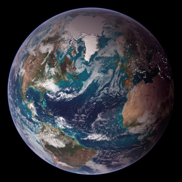
Approximately 71% of the Earth’s surface is covered by water. Moreover, well over 99% of the total heat budget of the earth is contained in the ocean. We have already seen how heat is the engine behind climate dynamics. It logically follows, therefore, that the oceans are an integral part of climate. In this section, we will focus on the physics of ocean circulation and how it helps drive climate. We will show that the effect on climate can be very large (including the whole ocean) or more regional, limited to an individual storm system. Finally, we will focus on the ways in which the ocean is likely to change in the future and how that change will have a profound impact on climate.
If you have spent time at the beach or in a coastal city, you will likely appreciate the way in which the ocean affects the weather and climate of the coastal region. Oceans have tremendously high heat capacity, so they have a large damping effect on climate. In the summer, the ocean acts to cool the land, and in the winter, the opposite effect occurs and the land is kept warmer. Take coastal California, for example. In the months of June and July, San Francisco is one of the coldest locations in the United States, yet in the winter, the city is among the warmest places. This dichotomy is a result of the effect of heat from the Pacific Ocean influencing the climate of the California coastline.
Goals and Learning Outcomes
Goals and Learning Outcomes
Goals
On completing this module, students are expected to be able to:
- describe surface and deep ocean properties;
- explain how surface and deep ocean circulation work;
- illustrate how ocean circulation affects weather and climate;
- predict changes in key ocean parameters and circulation patterns as a result of climate change;
- interpret deep sea circulation patterns from water column properties.
Learning Outcomes
After completing this module, students should be able to answer the following questions:
- What is the warmest temperature in the oceans today?
- What is the coldest temperature in the oceans today?
- What factors impact salinity of surface ocean waters?
- What is primary productivity and what controls it?
- What factors control dissolved oxygen contents of ocean waters?
- What factors control dissolved CO2 contents of ocean waters?
- What drives surface ocean circulation?
- What are the Coriolis effect, gyres, upwelling and downwelling?
- How do deep water masses form?
- What are the major deep water masses in the oceans and their properties?
- What is the significance of the Global Conveyor Belt, deep water aging, properties of the oldest waters in the ocean?
- What is ENSO?
- What are the impacts of ENSO on global weather patterns?
Assignments Roadmap
Below is an overview of your assignments for this module. The list is intended to prepare you for the module and help you to plan your time.
| Action | Assignment | Location |
|---|---|---|
| To Do |
|
|
Study of the Oceans
Study of the Oceans
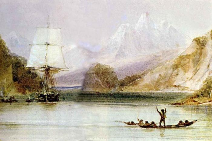
Humans have been involved in the scientific study of the ocean for hundreds of years. Most early ocean voyages were focused on exploration, colonization and economic gain. However, these early pioneers had to have an understanding of the ocean to survive their time at sea. It wasn’t until late in the 19th century that expeditions had the single goal of learning about the ocean. Charles Darwin’s famous five-year voyage on the HMS Beagle from 1831 to 1836 provided a literal treasure trove of information about the ocean and especially its geology and natural history. The HMS Challenger Expedition from 1872-1876 made even more important discoveries about oceanography.
World War II from 1939-1945 ushered in a new era in ocean exploration. The importance of naval operations, and particularly submarines in combat, provided a major incentive for a much more accurate understanding of the bathymetry of the ocean as well as the acoustic properties of seawater. The urgency of acquiring this information intensified in the Cold War interval from 1946 to 1991 when submarines played a central role in covert operations. Around the world, federal investment in oceanographic research ballooned, and research ships were built with the sole purpose of mapping the oceans and studying their properties. This age brought major discoveries of the ocean and its geology, the life it supports, its chemistry, and its effect on climate.
The scientific discovery of the oceans was originally focused on ships, but more recently our technological capabilities have surged, and now submersibles and unmanned remotely operated vehicles (ROVs) and autonomous underwater vehicles (AUVs) provide a relatively low operating cost means of acquiring many different types of data.
Examples of Submersibles
This technology is changing the way that oceanography is being conducted, as demonstrated in the following video. Click play to watch the video.
Video: Tethys - A new breed of undersea robot (2:03)
Tethys is a new breed of underwater robot developed at the Monterey Bay Aquarium Research Institute. Tethys is an autonomous underwater vehicle or an AUV. AUVs are programmed at the surface then released to follow a path beneath the ocean, collecting data as they go. Unlike existing AUVs, Tethys can travel rapidly for hundreds of kilometers, hover in the water for weeks at a time, and carry a wide variety of instruments. In designing this an AUV we were trying to make a fundamental change in how we do oceanography. Tethys is designed to travel to a spot in the ocean and park there until something interesting happens. If an algal bloom occurs, Tethys can move fast enough to follow the bloom and watch it evolve the way a biologist on land might follow and study a herd of deer. Tethys is small enough and light enough that it can be launched from a small boat at relatively low cost. In October 2010 we use Tethys for the first time to track patches of microscopic algae, as they were carried around Monterey Bay by the ocean currents. Tethys was created to be as energy efficient as possible, with a custom-designed hull, motor, and propeller. Like a fish, it can control its buoyancy and the angle at which it swims through the water. Tethys can dive hundreds of meters below the ocean surface and travel up to a meter per second. This is four times faster than existing long range vehicles, which allows Tethys to react more rapidly to changes in the ocean. While Tethys is at sea, we can monitor its progress from shore using computers or even cell phones. We can also view the data that the robot has collected. We're still in the testing phase, but our hope is that this little robot will eventually be able to travel all the way from California to Hawaii on a single set of batteries. This is Jim Bellingham for the Monterey Bay Aquarium Research Institute.
At the same time, satellites provide continuous information about the ocean surface, while data such as temperature and surface current velocity is obtained from long-term deployments of instruments attached to buoys. In addition, seismological data are acquired by seismometers anchored on the sea bottom. Nevertheless, modern oceanography still relies heavily on sea-going vessels for sampling waters and biotas from plankton to fish, for deploying instruments that measure in-situ properties, and for taking cores. We have already learned about such coring techniques in Module 1.
Data Collection Technologies
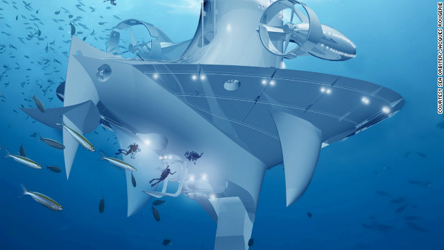
In the future, seagoing research vessels are likely to be extremely high-tech. For example, the SeaOrbiter is due to launch in the near future. Part giant ship and part giant submarine, the vessel will enable study of the sea surface simultaneously with its depths. One of the goals of the SeaOrbiter is to allow scientists to remain at sea and study underwater for extended periods, a pursuit not possible in a traditional submarine.
Check Your Understanding
Surface Water Properties
Surface Water Properties
We begin this module with an overview of the properties of seawater and follow with a thorough discussion of the circulation of different water masses.
Most of you have spent time at the beach or taken a boat trip from the coast. The realm that you have seen is the surface layer of the ocean. This is the warm, generally illuminated layer that is exchanging heat and gases with the atmosphere. The surface layer extends down usually a few hundred meters and accounts for only a small fraction of the total ocean volume. As such, it is very much like the skin of a piece of fruit. Yet this layer is home for much of the marine food chain. At the base of the surface ocean, is a sharp temperature drop at a layer known as the thermocline. Below the thermocline, ocean deep waters, by contrast, are generally cold, dark, and inhospitable. However, the deep ocean plays a vital role in heat transport, and thus we will spend considerable time considering deep-water masses.
Temperature
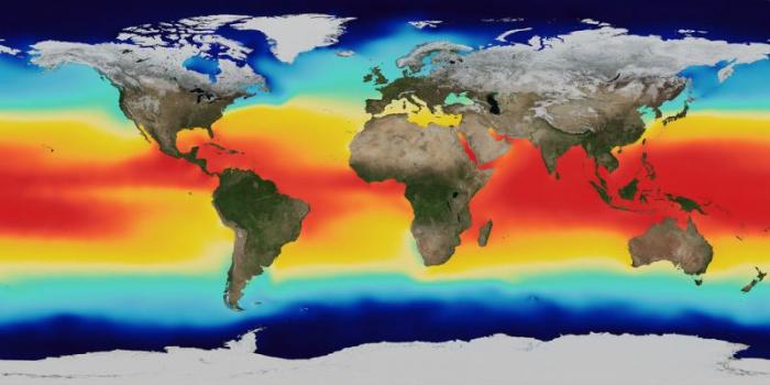
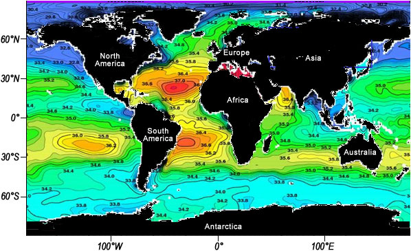
In terms of climate, the key property of seawater is its temperature. Temperature levels also help define the surface and deep ocean masses. Temperature of the surface ocean water varies seasonally, with warmer temperatures recorded in summer and colder temperatures in winter. When we study ocean temperatures, we usually consider the annual average. On this basis, surface ocean temperatures range from about 28oC in the tropical western Pacific to –3oC off the coast of Antarctica. Because seawater is salty, it does not freeze even though its temperature is below 0oC.
The following video shows real sea surface temperature data as well as the distribution of ice from 1985 to 1997. Note the way temperature bands and ice sheets shift from south to north with the seasons.
Video: 22 Years of Sea Surface Temperatures (1:47) This video is not narrated.
Temperature has a major influence on the density of seawater and thus plays a large role in deep ocean circulation, as we will see. Warm water expands and thus is less dense (less mass per unit area) than cold water.
Salinity
A key property of seawater that also has a significant effect on the behavior of water masses is salinity. This variable is a measure of the amount of dissolved salts such as sodium, potassium, and chlorine in the water, and, like temperature, it has a major effect on seawater density. The higher the salinity (the more salt), the denser the seawater. The major factor that controls salinity at a location is the balance of evaporation and precipitation. Where evaporation is higher than precipitation, salinity levels are higher; where precipitation exceeds evaporation, salinity levels are lower. The units of salinity are parts per thousand (ppt or o/oo), which refers to the weight of dissolved salt (in grams) in 1000 grams (or a kilogram) of water. The most saline surface waters are found in basins in highly arid regions with high rates of evaporation, such as the Persian Gulf, the Red Sea, and the eastern Mediterranean. Lowest salinities are found in locations with high levels of precipitation and runoff from land, typically near where large rivers enter the ocean. Highly saline water has more salt contained between the water molecules, and thus is denser than low salinity water.
Surface Ocean Circulation
Surface Ocean Circulation
The circulation of the surface ocean is driven primarily by surface winds. As we have seen, winds blow from areas of high atmospheric pressure to regions of low atmospheric pressure. These winds are generally transferring heat from areas where there is excess incoming radiation (the tropics and subtropics) to temperate and higher latitude regions, where there is a net loss of heat. Typically speaking, the distribution of pressure on the Earth’s surface is zonal or meridional, with high-pressure bands covering the subtropics and polar regions and low-pressure bands, the equatorial regions, and subpolar regions.
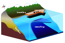
Where winds and surface currents are moving along a coastline, they draw the surface water away from the coast. The surface waters are replaced by waters from below by the upwelling described earlier. This is shown in the figure below.
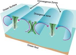
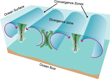
Upwelling also happens in parts of the ocean where winds cause surface currents to diverge or move away from one another. Downwelling is the opposite process to upwelling, where surface waters flow downwards and replace deep waters. This occurs in parts of the ocean where surface winds are converging. One place this happens is in the centers of gyres.
Check Your Understanding
The Coriolis Effect
The Coriolis Effect
Winds generally blow out from the subtropics towards the equator and subpolar regions, and from the polar regions to the subpolar latitudes. Complicating matters is that the rotation of the Earth causes the winds to rotate as they move (the Coriolis effect). The rotation of the Earth causes an object to deflect towards the right (as viewed by a stationary observer) in the Northern Hemisphere, which results in a clockwise motion, and to deflect towards the left (as viewed by a stationary observer) in the Southern Hemisphere, which results in a counterclockwise motion. These rotations combined with the zonal distribution result in enormous, nearly ocean-scale major cells or gyres of surface winds.
Video: Coriolis Effect (1:00)
The Coriolis force is the deflection of objects observed in a rotating reference frame. If a person is standing in a fixed position in the Northern Hemisphere, an object moving away from him or her will tend to rotate towards the right in the Northern Hemisphere, and the left in the Southern Hemisphere, as a result of the rotation of the earth. This effect is called the Coriolis force. The Coriolis force is very small because the rotation of the earth is very slow, 360 degrees in one day. However, the Coriolis force affects all air masses whether they be giant hurricanes, such as Hurricane Katrina here, with a rotation towards the right and clockwise, because it is in the Northern Hemisphere, cyclones, typhoons, as well as the large ocean gyres.
Major Surface Wind Maps
Gyres
Gyres
Video: Gyres (1:04)
Surface ocean currents are driven by surface wind patterns. For example, the trade winds in the tropics and the westerlies in the mid-latitudes. The trade winds in the tropics drive surface currents from the east towards the west, and in return, the westerlies drive surface currents from the west back towards the east. In addition, the Coriolis force results in gyres, rotational systems in each of the ocean basins that are clockwise in the Northern Hemisphere, for example, the North Atlantic gyre, and counterclockwise in the Southern Hemisphere, for example, the South Atlantic gyre. These gyres move warm waters from the south towards the north and in addition, they move cool waters from the north towards the south. Each gyre has a major effect on ocean circulation in that part of the ocean basin.
As surface winds push the surface layer of the ocean with them, the surface wind gyres result in surface ocean current gyres. Along coastlines, the direction of movement of a gyre has a significant impact on continental climate. For example, a current moving from south to north in the Northern Hemisphere, or north to south in the Southern Hemisphere, will generally deliver warmer water to the coastal region, whereas a current moving from the north to south in the Northern Hemisphere or south to north in the Southern Hemisphere will generally deliver colder water. The flow of warm water will generally cause a larger moderating influence on coastal climate than will the flow of cold water. Take, for example, the Gulf Stream in the North Atlantic. This warm current has a major heating effect on the shores of Great Britain and other parts of Northern Europe, keeping these regions relatively balmy compared to locations at comparable latitudes. After it bathes the shores of Britain, the North Atlantic gyre bends towards the south, thus bringing relatively cold waters to the shores of Spain, Portugal, and Morocco further to the south, keeping these areas cooler than areas not influenced by the currents.
This NASA video provides an excellent summary of surface ocean currents:
Video: Perpetual Ocean (3:02) This video is not narrated.
Major Deep Water Masses
Major Deep Water Masses
The deep ocean is generally considered to include the ocean below a transition known as the thermocline. The thermocline is the sharp temperature decrease that lies at the base of the surface mixed layer, where waters are generally uniform in temperature as a result of convection. Deep-water masses are produced at the surface of the ocean and transported to depth via downwelling. Generally, downwelling occurs where the surface ocean is cool, or, rarely, unusually saline. Downwelling water travels along lines of equal density known as isopycnals and spreads out horizontally at the level where it is equal in density to the surrounding water mass.
The production of deep-water masses via downwelling occurs in high-latitude regions of the northern and southern hemispheres, where the surface ocean is cooled by winds. Wind moving over the water both cools it and causes an increase in evaporation. This evaporation targets just the water molecules, resulting in an increase in the salinity of the water. Falling temperature and increasing salinity render these surface water masses denser, allowing them to downwell. In certain locations, the formation of sea ice also causes an increase in salinity as the freezing removes fresh water, leaving the salt behind in a process known as brine exclusion. Pockets of salty water around the margins of the ice sink as a result of their higher density. Moreover, brine exclusion intensifies the cooling by wind.
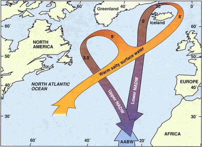
Today there are three major deep ocean masses. North Atlantic Deep Water or NADW is mainly produced where the surface ocean is cooled in the Norwegian Sea in the northern part of the North Atlantic on the north side of a ridge that runs between Greenland, Iceland, and Scotland. This cooled water seeps through the ridge and downwells. Portions of NADW are also produced in the Labrador Sea and in the Mediterranean. This water mass is 1-2.5oC and 35 ppt. NADW travels down the west side of the North Atlantic Ocean at a depth of 2000-4000m and through the west side of the South Atlantic. Much of NADW upwells in the Southern Ocean, but portions join the Antarctic Circumpolar Current and travel at depth into the Indian and Pacific Oceans.

Antarctic Bottom Water or AABW is produced by evaporative cooling off the coast of Antarctica and under the Ross ice shelf. With this source, AABW is amongst the coldest water in the ocean with a temperature of -0.4oC. This water is relatively fresh (average 34.6 ppt). AABW travels northward along the western side of the South Atlantic underneath NADW. Some of the water mass spills over into the eastern part of the South Atlantic, while the remainder travels into the equatorial channel between South America and Africa.
The third major source of deep water is called Antarctic Intermediate Water or AIW. AIW is produced near the Antarctic Convergence or Polar Front, where downwelling occurs as a result of the convergence of surface currents. AIW has a temperature of 3-7oC and a salinity of 34.3 ppt. It travels a considerable distance northward into the Atlantic, Indian and Pacific Ocean basins.
Other Deep Water Masses
Other Deep Water Masses
There are numerous other deep water masses, especially at intermediate depths, for example, North Pacific Intermediate water. As deep-water masses travel through the ocean, they gradually mix with surrounding water masses. For example, NADW mixes with AABW and AIW.
Downwelling supplies oxygen to the deep ocean and therefore ventilates this body of water. It does not bring nutrients. Deep water currents generally move very slowly, with a velocity of several cm per second. Typically, surface currents move 10-100 times faster than this. At these rates, deep water currents take thousands of years to encircle the globe. In fact, the oldest deep water in the ocean (in the North Pacific) is about 1500 years old. As deep waters circle the globe, their properties change. They mix with waters around them, and their chemistry changes as they acquire nutrients such as phosphate and CO2 from decaying organic matter and lose oxygen.
The opposite process of downwelling is upwelling. Upwelling is where a deep-water mass that is lighter than waters around it rises to the level where it is no longer buoyant. This situation generally results when surface winds move the surface water masses away from a location, resulting in the upward movement of water from depth to fill the void. Upwelling is frequent in coastal regions, especially those in subtropical regions, where high pressure results in a dominant offshore wind flow. In addition, the ocean divergences where winds move surface current by Ekman transport are frequented by upwelling. Upwelling is crucial to the supply of nutrients to surface water masses, fueling high levels of productivity in the surface ocean. The most prolific fisheries of the world in coastal regions occur in nutrient-rich waters such as Peru and California and are supplied by upwelling.
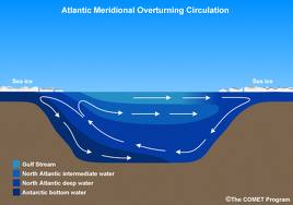
As we have seen, the circulation of the deep ocean is driven by density differences that arise as a result of temperature and salinity of the different water masses. This type of circulation is known as thermohaline (temperature=thermo; haline=salt or salinity). Strictly speaking, since surface ocean currents are not driven by thermohaline mechanics but by winds and to a much lesser degree, tides, the circulation of the ocean as a whole is often called the meridional overturning circulation. However, we will continue to use the term thermohaline when addressing deep-water circulation.
Check Your Understanding
Dissolved Nutrients
Dissolved Nutrients
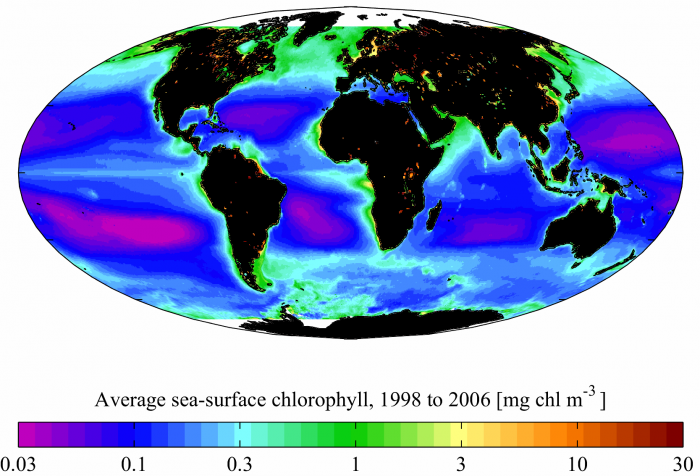
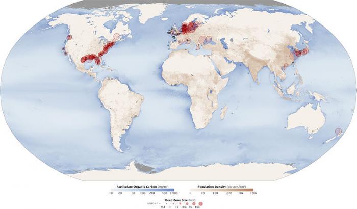
Probably the most important property of seawater in terms of its effect on life in the oceans is the concentration of dissolved nutrients. The most critical of these nutrients are nitrogen and phosphorus because they play a major role in stimulating primary production by plankton in the oceans. These elements are known as limiting because plants cannot grow without them. However, there are a number of other nutrients that also play a role, including silicon, iron, and zinc. Nutrients in the ocean are cycled by a process known as biological pumping, whereby plankton extract the nutrients out of the surface water and combine them in their organic matrix. Then, when the plants die, sink and decay, the nutrients are returned to their dissolved state at deeper levels of the ocean. The abundance of nutrients determines how fertile the oceans are. A measure of this fertility is the primary production, which is the rate of fixation of carbon per unit of water per unit time. Primary production is often mapped by satellites using the distribution of chlorophyll, which is a pigment produced by plants that absorbs energy during photosynthesis. The distribution of chlorophyll is shown in the figure above. You can see the highest abundance close to the coastlines, where nutrients from the land are fed in by rivers. The other location where chlorophyll levels are high is in upwelling zones, where nutrients are brought to the surface ocean from depth by the upwelling process.
Another critical element for the health of the oceans is the dissolved oxygen content. Oxygen in the surface ocean is continuously added across the air-sea interface as well as by photosynthesis; it is used up in respiration by marine organisms and during the decay or oxidation of organic material that rains down in the ocean and is deposited on the ocean bottom. Most organisms require oxygen, thus its depletion has adverse effects for marine populations. Temperature also affects oxygen levels, as warm waters can hold less dissolved oxygen than cold waters. This relationship will have major implications for future oceans, as we will see.
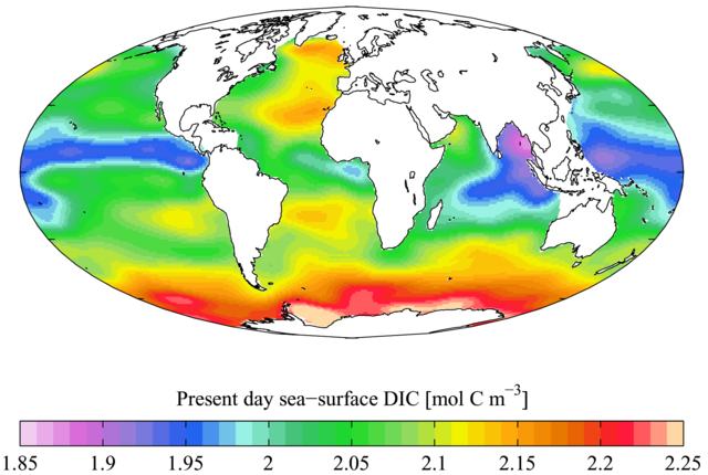
The final seawater property we will consider is the content of dissolved CO2. CO2 is nearly opposite to oxygen in many chemical and biological processes; it is used up by plankton during photosynthesis and replenished during respiration as well as during the oxidation of organic matter. As we will see later, CO2 content has importance for the study of deep-water aging.

Dissolved CO2
Check Your Understanding
The Global Conveyor Belt
The Global Conveyor Belt
As we have seen, surface ocean currents are the dominant sources of deep water masses. In fact, it is a little more complicated than this, as other deep water masses also feed one another. However, in a generalized sense, the surface and deep ocean currents can be viewed as an integrated system known as the Global Conveyor Belt, a concept conceived by the brilliant Geoscientist Wally Broecker of Columbia University. Diagrams of the Global Conveyor Belt (GCB) are two-dimensional and therefore simplified and do not, for example, include all of the intermediate water masses or surface water currents. However, the key of the Global Conveyor Belt concept is that it explains the general systems of heat transport as well as bottom water aging and nutrient supply in the oceans.
Global Conveyor Belt
The following animation traces the path of water through the surface and deep ocean, showing the dominant features of the GCB, including formation of NADW in the North Atlantic.
Video: The Thermohaline Circulation - The Great Ocean Conveyer Belt (2:46) This video is not narrated.
The GCB shows the dominant source of deep water in the oceans as North Atlantic Deep Water, and how this splits in two to flow into the Indian and Pacific Oceans. In these locations, upwelling of the deep water mass produces surface water currents that generally flow back towards the original source of deep water in the North Atlantic. For heat supply, the conveyor belt involves the transport of heat and moisture to northwest Europe by the Gulf Stream; this accounts for about 30% of the heat budget for the Arctic region, making the GCB extremely important for climate in the Arctic.
Because deep-water masses circulate very slowly, the GCB takes about 1500 years to complete, meaning that the oldest water in the oceans is about this age. In addition, because oxygen is gradually depleted in deep waters as they age, and because CO2 contents and nutrients conversely increase, the oldest water masses of the ocean in the North Pacific are among the most nutrient-rich, CO2 rich, and oxygen-depleted waters in the ocean. Conversely, the newly produced NADW waters are among the most nutrient-depleted, CO2 depleted, and well-oxygenated waters in the world.
As it turns out, recent research on the detailed configuration of surface and deep currents shows that circulation is much more complex than the GCB. Floats deployed in the ocean don’t always follow expected pathways in the GCB model. Wind actually plays a more significant role in causing downwelling than previously thought. Moreover, mixing by small systems or eddies plays a large role in driving surface currents.
Check Your Understanding
El Niño-Southern Oscillation (ENSO)
El Niño-Southern Oscillation (ENSO)
Overview
El Niño, the most powerful control on weather across the planet, is rearing its ugly head as we speak. The telltale signs are building, and atmospheric scientists are predicting one of the most powerful El Niño events in history, certainly the strongest since 1998. This actually could be very good news for drought-stricken California, as El Niño typically delivers a lot of rain and snow to the state. In the case of California, the drought has been so severe that rains last winter caused massive mudslides. And the rain caused so much new vegetation to grow, and this served as fuel for the fires in Summer 2017. Southern Australia becomes very dry in El Niño years, and the drought causes great hardship for farmers and can often lead to very dangerous bushfires. And in Peru, El Niño comes with changing ocean currents that lead to the collapse of fisheries and great financial hardships. In this section, we learn about ocean circulation and how it impacts climate on a global scale.
One of the clearest examples of the influence of the oceans on climate is the El Niño Southern Oscillation (ENSO). This is the strongest inter-annual (i.e. periodic) variation in the modern climate system. The ENSO cycle lasts between two to seven years (average of 4 years) and corresponds to sea surface and thermocline temperatures and atmospheric pressure changes in the Pacific Ocean that ultimately have effects on weather and surface ocean conditions across the globe. The ENSO cycle consists of two main climatic intervals, the El Niño interval and the La Niña interval. The El Niño stage begins with an increase in sea surface temperatures across the eastern Pacific as warm waters spread from the west.
Typically, there is a very large east to west SST gradient across the Pacific, but El Niño virtually erases this gradient. For reasons that are not fully understood, the El Niño stage is characterized by high atmospheric pressure in the western Pacific. The opposing La Niña stage is characterized by relatively cool waters in the eastern tropical Pacific and low atmospheric pressure in the western Pacific. The westward trade wind flow piles up warm water in the western Pacific and this causes sea level to be higher by about 20 cm in the western compared to the eastern Pacific (so sea level is, relatively speaking, higher in the eastern Pacific during El Niño). To compensate for this wind flow, the thermocline slopes down upwards towards the eastern Pacific, resulting in greater stratification in the east. The slope of the thermocline shallowing changes markedly during ENSO. As El Niño piles up warm water in the eastern Pacific, the thermocline deepens in that location, whereas the La Niña part of the cycle corresponds to a very shallow thermocline in the eastern Pacific.
The following animation shows how an El Niño event in 1997 developed in the tropical Pacific Ocean:
Video: Visualizing El Niño From NASA Scientific Visualization Studio (2:28)
El Niño, the world's biggest climate phenomenon, returned stronger than ever in 1997. Satellite, ship, and buoy observations show the onset of this warming of the eastern Pacific Ocean as early as May. El Niño globally changes precipitation and temperature patterns, often with destructive results.
Visualizing how three key datasets differ from normal conditions reveals the magnitude of the 1997-98 event and gives new insights into how the ocean and atmosphere couple to produce El Niño. First, we look at sea surface height. The gray sheet rises and dips as much as 30 centimeters from normal. Next, we map sea surface temperature. Red is 5 degrees Celsius above normal and blue 5 degrees below normal. Finally, black arrows are added to mark sea surface winds.
A weakening of the trade winds in the far western Pacific fuels an eastward moving wave. Sea level is raised as the windswept wave progresses. The waves arrival at the South American coast reduces the normal upwelling of cold water and warms the surface by as much as five degrees Celsius. Intense atmospheric convection associated with equatorial ocean warming causes local winds to converge, abating the trade winds strength and extending the warm pool of water into the eastern Pacific. Beneath the ocean surface, warm and cold waters are separated by the thermocline, a boundary at 20 degrees Celsius. El Niño flattens the thermocline, squeezing the warm bulge of water eastward into a long, shallow pool. As scientists collect more detailed data through efforts such as NASA's Earth observing system, visualization will be crucial in probing the elaborate interactions and far-flung effects of future El Niños.
As you may recall from Module 2, there is a good correlation between El Niño events and warmer temperatures on a global scale; in fact, a good part of the temperature variation superimposed on the general warming trend of the last 60 years can be explained by ENSO variability. This can be seen in the figure below (from Module 2).
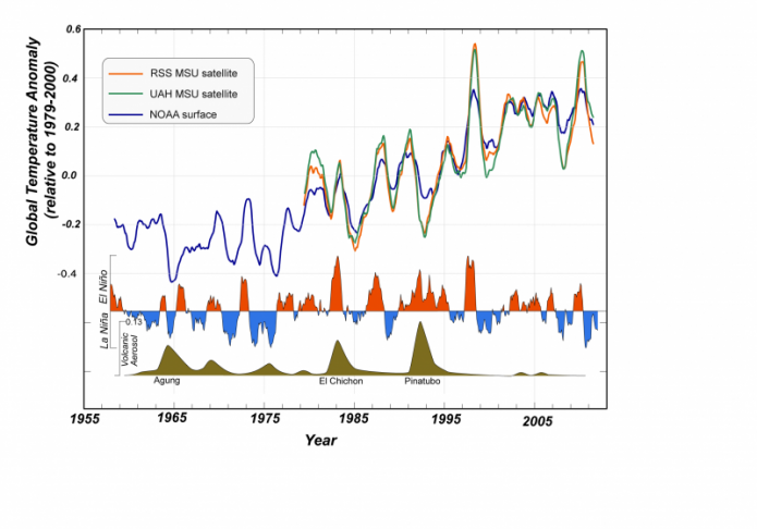
During an El Niño event (red parts of the ENSO curve), more water vapor is added to the atmosphere, making it warmer, and during a La Niña event (blue parts of the ENSO curve), less water vapor makes it into the atmosphere, so the global temperature drops. Remember that water vapor is a greenhouse gas, and it also transports heat to the atmosphere when the vapor condenses to form water droplets (clouds and rain).
ENSO has major implications on weather across the globe. For example, drought conditions in 2012 in the Midwest are a direct result of the ENSO cycle. El Niño intervals correspond to increased precipitation in California and eastern South America, due largely to the ability of warm water to hold more moisture than cold water. The warm surface water in the eastern Pacific also increases surface ocean stratification and decreases upwelling offshore Peru and Ecuador. The implications of diminished upwelling are severe for coastal fisheries in these countries. Warm water also increases the occurrence of bleaching in the Caribbean and eastern Pacific corals. The position of the high-pressure region in the Pacific affects the tracks of Pacific cyclones. In the Atlantic, increased wind shear during El Niño intervals inhibits the formation of hurricanes. El Niño intervals also correspond to cooler and wetter winters in Florida and the southeastern US, and warmer and drier winters across the northern tier of the US and in Canada. The La Niña phase corresponds to the opposite conditions from El Niño, most notably an increase in the frequency in Atlantic hurricanes as conditions become more favorable for their formation (i.e., less shear in the tropical Atlantic).
Check Your Understanding
Ocean Futures
Ocean Futures
Overview
Since records have been kept, the average temperature of the global surface ocean has warmed by more than 1oC. Models suggest that all areas of the surface ocean will warm significantly more than this by 2100, especially in the high latitudes. This warming will have major implications for a number of key processes in the oceans, some of which will impact climate and weather patterns on land. In this section, we discuss the impact of climate change on the intensity and frequency of hurricanes, the potential shutdown of the global conveyor belt, the intensity of the ENSO cycle and the occurrence of oceanic hypoxia.
Hurricanes
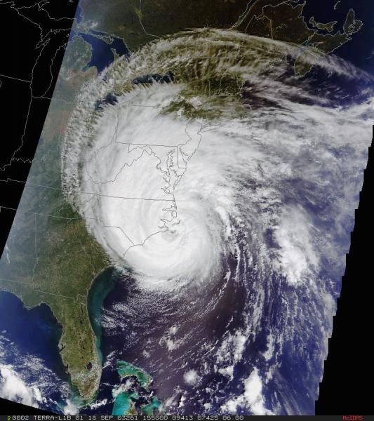
Many of you learned about the devastating force of hurricanes when Katrina hit New Orleans in August 2005. In fact, there have been a number of devastating hurricanes over the last few decades with Hurricane Hugo (Charleston) in 1989, Hurricane Andrew (South Florida) in 1992, and Typhoon Yasi in the Pacific (Australia) in 2011. Atlantic Hurricanes and Cyclones in the Pacific Ocean get their energy from the warm tropical ocean, so wouldn’t it follow that a warmer ocean will fuel more deadly hurricanes? Well, it’s not quite that simple and is more than a little controversial.
Early in spring, Bill Gray from Colorado State University puts out an annual hurricane forecast for the late summer and fall Atlantic Hurricane season. Gray’s forecast is based on a number of factors including sea surface temperatures in the tropical Atlantic, a number of atmospheric parameters, and the stage of the ENSO cycle. While hurricane experts agree about the feasibility of season forecasting, there is much less consensus among them about the effect of climate change on storms. Part of the problem is that coupled climate-ocean models do not have the resolution to forecast storms with a great deal of accuracy.
Since 1980 there has been a marked increase in the SSTs in the tropical Atlantic from August to October, the interval when hurricanes are formed, and the maximum power dissipation of hurricanes, which is the product of the summed maximum wind speed cubed and its duration. In fact, the agreement between these parameters is exceptional. Yet over the same time period, there is no observed increase in the frequency of hurricanes. In fact, when climate modelers downscale models of future climate to attempt to observe predictions for smaller regions than models typically yield, the result is a prediction of increased hurricane intensity but actually fewer storms in the future.
Global Conveyor
As we have seen earlier, the North Atlantic Ocean is the central driver of the global conveyor. Changes in density of surface waters in the Norwegian Sea as a result of warming, increased precipitation and melting of Greenland Ice can impact the flow of water downwelling as NADW. Sufficient changes in density could potentially shut down the production of NADW and literally halt the global conveyor. This, in turn, would have major implications for global climate.
You might find it hard to believe that such a massive engine of water and heat transport could possibly shut down. However, it has happened numerous times in the past, and this is perhaps the strongest evidence that it could happen in the future. Moreover, the past shutdowns have occurred over very short time intervals. Here, we will summarize our current understanding of the likelihood of GCB shutdown.
Approximately 8200 years ago, in the midst of the gradually warming climate of the current interglacial, a very abrupt cool period occurred that was likely the result of rapid melting of the Northern Hemisphere ice sheet and the flow of massive amounts of freshwater into the North Atlantic Ocean. The event was about 10-15 years long---a geologic heartbeat---and was likely due to a massive breach of the meltwater over a barrier in the St Lawrence Seaway. The impact of the flood of freshwater across the surface of the North Atlantic Ocean was to decrease the density of the water to such an extent that downwelling virtually stalled. The switching off of thermohaline circulation drastically slowed oceanic heat transport, which in turn led to rapid cooling in the Northern Hemisphere, especially in Northern Europe.
Moving on to the present day, flow of NADW is likely weakening due to increasing SSTs and freshening of the North Atlantic. Freshening is the result of melting of Greenland ice, as well as increased moisture transport in a warmer atmosphere. However, detection of a slowdown is very difficult as the meridional overturning circulation is highly variable, with a yearly average of 18.7 Sverdrup (a Sverdrup is one million m3 per second), but a range of 4.4 to 35.3 Sverdrup. Weakening is likely to continue into the future, also as a result of increased precipitation in northern high latitudes. However, most coupled ocean-models suggest that under realistic emission scenarios, thermohaline circulation will continue to slow but not shut down. The consensus of model runs suggests reductions of 10-50% in meridional overturning circulation intensity in the year 2100. However, these predictions are somewhat difficult because the relationships between many of the variables are not linear, rather there appear to be thresholds or tipping points that make prediction difficult.
What does this weakening of the NADW mean for the climate? Most ocean models show that as it weakens, less of the Gulf Stream warmth travels to high latitudes. Today, this warmth accounts for something like 30% of all the heat supplied to the Arctic region, so as the NADW weakens, models predict less heat moving into the Arctic. This might lessen the expected dramatic warming in the Arctic, but if it slows too much, there is a chance that the Arctic could become much colder — and very rapidly — as it did during the Younger Dryas event about 11 thousand years ago.
ENSO
The connection between climate change and changes in the duration and intensity of ENSO events has been hotly debated as the relationship of extreme weather events (often connected to ENSO) and climate change has been debated. Are extreme events getting more extreme as a result of climate change or is this just a part of the normal ENSO variability? Examples include major blizzards in the northeastern US during La Niña years and intense “Pineapple Express” rainfall in California during the El Niño stage of the ENSO cycle. As easy as it is to attribute such extreme events to climate change, reality is not nearly that simple, as these events fall under weather and not climate and much longer-term changes are required before an empirical connection can be made with certainty.
Models do not agree on the effects of warming on the ENSO cycle and so we will have to wait to see what happens in the future.
Ocean Dead Zones or Hypoxia
Another great threat to marine environments is hypoxia, a condition in which seawater or freshwater becomes deficient in oxygen. As with harmful algal blooms, the main culprit for hypoxia is nitrification from agriculture or pollution. This oxygen deficiency can cause massive fish kills that can devastate coastal economies. Since warm waters can hold less oxygen than cold waters, climate change will render coastal regions more prone to hypoxia in the future. Hypoxia tends to occur when waters become increasingly stratified, which is gradually occurring in many coastal areas.
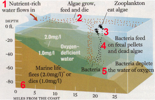
The northern Gulf of Mexico is a region where a seasonal dead zone is now well established. This dead zone was first noted in the 1970s and has gradually grown in size and intensity since. The critical driver for hypoxia is the outflow of nutrients from the Mississippi River. The Mississippi drains an enormous agricultural region of the mid-continent and thus acquires a very high level of nutrients. These spur production by algae in the surface ocean, which in turn rains down and utilizes oxygen in the deeper water column. The dead zone appears in spring as nutrient loads increase and peaks in late summer as oxygen becomes steadily depleted, exacerbated by the fact that warmer waters hold less oxygen than colder waters. Other regions with prominent dead zones include the Chesapeake Bay and Long Island Sound in the US and the Baltic Sea in Northern Europe. These areas will be more prone to hypoxia in the future.
The following video gives an overview of how hypoxia develops in the Gulf of Mexico.
Video: Gulf of Mexico Dead Zone (3:50) This video is not narrated.
The Dead Zone
Nutrient Runoff Creates Hypoxia in the Gulf of Mexico
Data provided by: Maria A. Faust (Smithsonian Institution)
Katja Fennel (Dalhouse Univ)
Robert Hetland (Texas A&M)
Phytoplankton
Did you know that half of the oxygen that we breathe comes from tiny organisms that live in the ocean? It’s true! These microscopic marine organisms called phytoplankton, produce oxygen just like land plants. But phytoplankton are not plants, they are Protists, single celled organisms. They are so small that thousands of them can fit in a single drop of water. In order to study phytoplankton, scientists often use microscopes or satellites.
From space we see Earth like this… but some satellites see Earth like this… a dance of rainbow colors. In this case the colors represent the concentration of phytoplankton in the oceans; red is high concentration; blue is low concentration.
Phytoplankton depend on nutrients and the proper temperature and light conditions to grow and reproduce. Coastal areas are extremely rich in nutrients, which have been washed off the land by rivers. Areas such as the open ocean have lower concentrations of phytoplankton because of the limited amount of nutrients there.
The mouth of the Mississippi River is a perfect example of how nutrient run-off creates plankton blooms. 41% of the United States drains into the Mississippi River and then out to the Gulf of Mexico. That’s a total of 3.2 million square kilometers of land, or about 600 million football fields. About 12 million people live in urban areas that border the Mississippi, and these areas constantly discharge treated sewage into rivers. However, the majority of the land in the Mississippi’s watershed is farm land. Each spring as farmers fertilize their lands preparing for crop season, rain washes fertilizer off the land and into streams and rivers. All of the urban and farm discharge includes nutrients such as nitrogen and phosphorus that are very important for the growth of phytoplankton. Incredibly, about 1.7 million tons of these nutrients are dumped into the Gulf of Mexico every year. Once the Gulf of Mexico receives this huge influx of nutrients, massive phytoplankton blooms occur. These blooms result in an area called the Dead Zone — areas with such low oxygen concentration that few organisms can survive there.
But if phytoplankton blooms produce oxygen, then why does a Dead Zone occur? For animals, such as microscopic zooplankton and fish, phytoplankton blooms are like an all-you-can-eat buffet. Small animals eat the phytoplankton, and are in turn eaten by bigger fish. All along, these animals are releasing waste, which falls to the bottom of the Gulf. There lurk bacteria that decompose the waste, and in the process use up the oxygen, creating hypoxic conditions. The different densities of fresh water from the Mississippi and salt water from the Gulf create barriers that prevent mixing between the surface and deep waters. Soon there is not enough oxygen for other organisms to use. The Dead Zone has arrived. But as summer turns to fall, winds help to stir up the water, allowing the layers to mix and replenish oxygen throughout the water. Eventually the Gulf and its fish population return to normal… until next year.
Check Your Understanding
Module Summary and Final Tasks
Module Summary and Final Tasks
End of Module Recap:
In this module, you should have grasped the following concepts:
- techniques used to study the oceans and their properties;
- distribution of the major properties (temperature, salinity, oxygen, nutrients) of surface and deep water and the processes that control them;
- the drivers of surface ocean circulation and how it impacts climate;
- the drivers of deep ocean circulation and the dominant deep water masses;
- upwelling and downwelling and how they impact ocean properties;
- El Niño Southern Oscillation and how it impacts global weather patterns;
- the global conveyor belt;
- likely changes in the ocean circulation in the future and how they will impact climate.
Assignments
You should have read the contents of this module carefully, completed and submitted any labs, the Yellowdig Entry and Reply, and taken the Module Quiz. If you have not done so already, please do so before moving on to the next module. Incomplete assignments will negatively impact your final grade.