
In addition to technology, economics also plays a role in the production of oil/gas in the sense that higher prices will motivate greater production. Let’s assume that the as the supply of proven reserves drops, the price will rise. As long as there is a demand for oil and gas, as it becomes more scarce, it will become more valuable. This is a pretty simplistic view of what determines the price of oil and gas — reality is much more complex, which is why prices fluctuate quite a bit over time. But it is hard to escape the basic reality that as a desirable commodity becomes scarce, its value goes up.
To make this change in the model, we need to add something that will calculate the price. This new model looks like this:
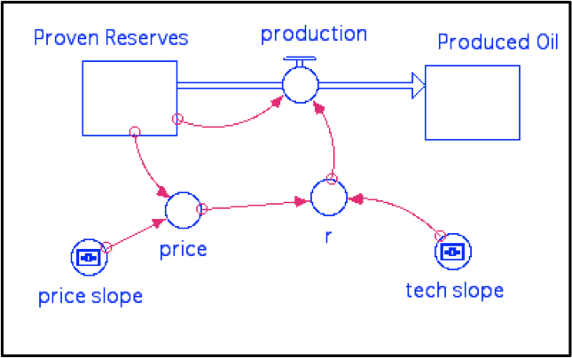
As before, production is defined as Proven Reserves x r, and r in this case is defined as price x tech_slope x TIME, so it once again has the increase over time that our previous model had, but it also increases as the price goes up. The tech_slope is just the slope of the increase in technology over time and the default value is 0.0002. Price here is defined as 0.01 + price_slope x (100 – Proven Reserves); price_slope is the slope of price increase relative to change in Proven Reserves, and is originally set to 0.05. At the beginning, Proven Reserves is 100, so this gives a price of 0.01 — very small. But, when Proven Reserves has declined to 50, we get a price of 2.51. This equation is not meant to be anything more than a way to make the price increase as the Proven Reserves get smaller. The value 0.01 at the front end of this equation is just there so that the price is not 0 at the beginning, which would then make r be 0 and no oil would ever get produced.
What we have created here is a system with a feedback mechanism. Here is how it works:

If the production increases, then the proven reserves must decrease; this triggers an increase in price, which in turns triggers an increase in production. Notice that the starting point (production increase) and the ending point (production increase) are the same. In other words, the change at the beginning of the mechanism promotes more of the same — this is what is known as a positive feedback mechanism. Positive feedback mechanisms tend to cause an acceleration of change, sometimes resulting in runaway behavior. In contrast, the are other feedback mechanisms that tend to counteract change, encouraging stability; these are known as negative feedback mechanisms. Note that in this context, positive is not necessarily good, and negative is not necessarily bad.
Take a few minutes to watch the video below to learn more about the positive feedback mechanism the oil production model before running the next model.
Video: Peak Oil Positive Feedback (1:19)
This simple diagram is meant to represent the positive feedback mechanism that we've put into the model. So if you imagine that we begin with a production increase. That's the initial change. Let's say something happens and we increase production. That is going to cause the proven reserves to decrease, right, because production drains that reservoir. So as that goes down, the commodity becomes more scarce and because of that, the price goes up. So that's another effect here that's triggered by the production increase. And as the price is increased, that will then encourage us to do even more to try to produce more of the oil that's out there. It's an incentive to produce more oil.
So that leads to an increase in production again. So the initial change that began this was the production increase and that has end up triggering a series of responses in the model that lead to a further increase in price, and so when that happens, this is called a positive feedback mechanism. It's kind of like a cause and effect loop, right. So here's a cause, it makes in effect, it makes an effect, makes another effect that comes back on that cause and enhances it. So that's going to really change the way that this model behaves.
Open the model here, and run it.
This model has two pages of graphs to look at; the first one shows the Proven Reserves, Produced Oil, price, and production, and r (which combines price and tech slope), while the second one shows just the production. The second graph retains the results from previous model runs, allowing you to make comparisons as you make changes to some of the adjustable model parameters. If you want to clear this graph, hit the Restore Graphs button.
| Practice | Graded | |
|---|---|---|
| Tech slope | 0.0001 | 0.0002 |
| Price slope | .05 | .07 |
Questions
3A. First, run the model as it is, with the price slope set to 0.05 and the tech slope set to 0.0002. Note the time and magnitude of the peak in production. Then alter the tech slope or price slope as prescribed, using the new values provided. Run the model and compare the peak time and magnitude with the original case (use page 2 of the graph pad). Use “sooner” or “later” and “greater” or “smaller” to describe how your alterations changed the timing and magnitude of the peak in production.
Change in time of peak =
Change in magnitude of peak =
a) Yes — there are just a few cases in which a peak occurs
b) No — it is impossible; the best you can do is a broad, low peak that takes a long time to develop.