Introduction to a Simple Planetary Climate Model
Introduction to a Simple Planetary Climate Model
Our first climate model calculates how much energy is received and emitted (given off) by our planet, and how the average temperature relates to the amount of thermal energy stored. The complete model is shown below, with three different sectors of the model highlighted in color:

First, let’s define a few terms that you might not be familiar with.
Insolation —stands for Incoming Solar Radiation, which is a fancy way of saying sunlight or solar energy.
Albedo — the fraction of light reflected from some material; 0 would be a perfectly black object (no reflected light) and 1 would be a perfectly white object (no light absorbed).
Heat capacity — this is the amount of energy (units are Joules) needed to raise 1 kilogram of some material 1°C.
Ocean Depth — this is the depth of the part of the ocean that is involved in climate over short time scales of decades, the part of the ocean exchanges energy with the atmosphere. While the whole ocean has an average depth of ~4000 m, the part we worry about here has a depth of less than 500 m.
LW Int and LW slope — these are parameters used to describe the relationship between the average planetary temperature and the amount of long-wavelength (infrared, or thermal) energy emitted by the planet; more details are provided below.
The Energy In Sector
The Energy In Sector
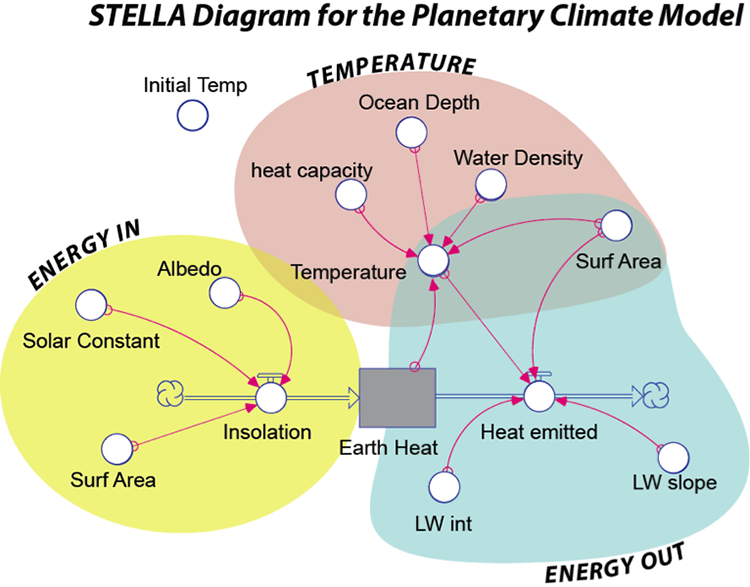
The Energy In sector (yellow in Fig. 1 above) controls the amount of insolation absorbed by the planet. The Solar Constant is not really a constant, but it does tend to stay close to a value of 343 Watts/m2 (think of about six 60 Watt light bulbs shining down on a patch of ground 1 meter on a side — this is what we get from the Sun). This is then multiplied by (1 – albedo) and then the surface area of the Earth giving a result in Watts (which is a measure of energy flow and is equal to Joules per second). In the form of an equation, this is:
S is the Solar Constant (343 W/m2), A is surface area, and α is the albedo (0.3 for Earth as a whole).
This is the equation Ein=S×A×(1-α)
The Energy Out Sector
The Energy Out Sector
The Energy Out sector (blue above) of the model controls the amount of energy emitted by the Earth in the form of infrared (thermal) radiation, which is a form of electromagnetic radiation with a wavelength longer than visible light, but shorter than microwaves. You saw earlier that this is often described using the Stefan-Boltzmann Law which says that the energy emitted is equal to the surface area times the emissivity times the Stefan-Boltzmann constant times the temperature raised to the fourth power:
A is the whole surface area of the Earth (units are m2), ε is the emissivity (a number between 0 and 1 with no units), σ is the Stefan-Boltzmann constant (units are W/m2 per °K4), and T is the temperature of the Earth (in °K). The problem with this approach is that it ignores the greenhouse effect, which is a very important part of our climate system. We could represent the greenhouse effect by choosing the right value for the emissivity in the Stefan-Boltzman law, but here, we will use a different approach, one in which Eout is based on actual observations. With a satellite above the atmosphere, we can measure the amount of energy emitted in different places on Earth and figure out how it relates to the surface temperature. As it turns out, this is a pretty simple relationship, described by a line:
Eout=(〖LW〗_int+〖LW〗_s×T)×A
The part inside the parentheses is just the equation for a line, with an intercept (LWint with units of W/m2) and a slope (LWs with units of W/m2 per °C). This new way of describing Eout is shown as the red line in the figure below:
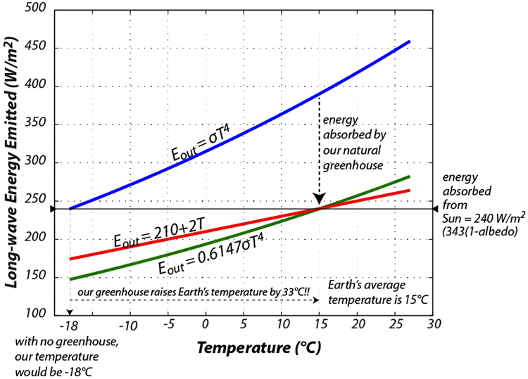
The key thing here is that the hotter something is, the more energy it gives off, which tends to cool it and it will continue to cool until the energy it gives off is equal to the energy it receives — this represents a negative feedback mechanism that tends to lead to a steady temperature, where Ein = Eout.
The Temperature Sector
The Temperature Sector
The Temperature sector (brown in Fig. 1) of the model establishes the temperature of the Earth’s surface based on the amount of thermal energy stored in the Earth’s surface. In order to figure out the temperature of something given the amount of thermal energy contained in that object, we have to divide that thermal energy by the product of the mass of the object times the heat capacity of the object. Here is how it looks in the form of an equation: (see directions for how view images in a larger format [1])
Let’s look at it with just the units, to make sure that things cancel out:
This can be simplified by combining, rearranging, and canceling to give:
Here, E is the thermal energy stored in Earth’s surface [Joules], A is the surface area of the Earth [m2], d is the depth of the oceans involved in short-term climate change [m], ρ is the density of seawater [kg/m3] and Cp is the heat capacity of water [Joules/kg°K]. We assume water to be the main material absorbing, storing, and giving off energy in the climate system since most of Earth’s surface is covered by the oceans. The terms in the denominator of the above fraction will all remain constant during the model’s run through time — they are set at the beginning of the model and can be altered from one run to the next. This means that the only reason the temperature changes is because the energy stored changes.
Other parts of the model
Other Parts of the Model
The model has a few other parts to it, including the initial temperature of the Earth, which determines how much thermal energy is stored in the earth at the beginning of the model run. It also includes some other features that allow you to change the solar input and the part of the greenhouse effect due to CO2. We use the standard assumption (which is itself based on some physics calculations) that for each doubling of the CO2 concentration, there is an increase of 4 W/m2 in the greenhouse effect. This is often called the greenhouse forcing due to CO2. In terms of our Eout curve shown in Figure 2 above, this shifts the red curve downwards — so less energy is emitted, and thus more is retained by the Earth. Let’s consider how this works — if we start with 200 ppm of CO2 and increase it to 800 ppm, that represents 2 doublings (from 200 to 400 and then from 400 to 800), so we would get 8 W/m2 of greenhouse forcing.
One unit of time in this model is equal to a year, but the program will actually calculate the energy flows and the temperature every 0.1 years.