Summative Assessment
Reminder!
After completing your Summative Assessment, don't forget to take the Module 10 Quiz. If you didn't answer the Learning Checkpoint questions, take a few minutes to complete them now. They will help your study for the quiz and you may even see a few of those questions on the quiz!
Modeling the Economics of Climate Change Activity
The global climate system and the global economic system are intertwined — warming will entail costs that will burden the economy, there are costs associated with reducing carbon emissions, and policy decisions about regulating emissions will affect the climate. In the language of systems thinking, this means that there are important feedback mechanisms in this system — a change in the economics realm will affect the climate realm, which will then influence the economics realm. These interconnections make for a complicated system — one that is difficult to predict and understand — thus the need for a model to help us make sense of how these interconnections might work out. In this activity, we’ll do some experiments with a model (a modified version of Nordhaus' DICE model mentioned earlier in this module) that will help us do a kind of informal cost-benefit analysis of emissions reductions and climate change. As with the other STELLA-based exercises you've done, this one will help you develop your abilities as a systems thinker.
Instructions
Read the following pages for an introduction to this model (this introductory material is also on the worksheet you download below) and then run the experiment using the directions given on the worksheet. As before, there is a practice version, with answers on the worksheet, and a graded version. Once you have completed the graded version and entered your answers on the worksheet, go to Module 10 Summative Assessment: Graded to enter your answers.
Files to Download
Download worksheet [1] to use when submitting your assignment
Submitting Your Assessment
Once you have answered all of the questions on the worksheet, go to Module 10 Summative Assessment: Graded. The questions listed in the worksheet will be repeated in this Canvas Assessment quiz. So all you will have to do is read the question and select the answer that you have on your worksheet. You should not need much time to submit your answers since all of the work should be done prior to starting the Assessment. The assessment is timed. You will have 40 minutes to complete it.
Grading and Rubric
| Item | Possible Points |
|---|---|
| Questions 1-8 | 1 point |
| Questions 9-10 | 3 points |
Activity: Modeling the Economics of Climate Change
Activity: Modeling the Economics of Climate Change
Video: Model Introduction(2:24)
For the module ten summative assessment, we're going to be working with this very large and complicated model, that consists of a number of different parts. You can see down in here this is the global carbon cycle and then that includes the percent or the concentration of CO2 in the atmosphere. That concentration of CO2 in the atmosphere then feeds into a climate model that tells us the temperature. And that temperature then goes into determining the sort of climate damages caused by a global temperature, global warming. Those climate damage costs then affect the amount of money that we have leftover to invest in the economy. So here's global capital - this is the whole kind of the heart of the economic model up in here. So climate damages come into play here. Another important cost that comes into play are the abatement costs. These are the costs related to reducing carbon emissions. And so there's something down here called the emissions control rate that we'll fiddle around with. It represents, essentially, different choices we make about how much we're going to try to limit carbon emissions. That limits how much goes in the atmosphere, it limits the temperature, and so on. But it costs money, so there's a certain abatement cost per gigaton of carbon that you are not emitting into the atmosphere. There are a whole bunch of other parts of this global climate and climate and economic model, including something that keeps track of what Nordhaus calls social utility. The global population here is sort of fixed and these are a bunch of things that just sort of sum up some of these economic components of the model. So this is the big model that's behind the scenes. When you look at the actual model, you'll be seeing something like this - an interface where you're just going to change a few basic things. And& for this summative assessment, we're really just going to change the emissions control rate here, which is a graphical function of time.
The global climate system and the global economic system are intertwined — warming will entail costs that will burden the economy, there are costs associated with reducing carbon emissions, and policy decisions about regulating emissions will affect the climate. These interconnections make for a complicated system — one that is difficult to predict and understand — thus the need for a model to help us make sense of how these interconnections might work out. In this activity, we’ll do some experiments with a model that will help us do a kind of informal cost-benefit analysis of emissions reductions and climate change.
The economic part of the model we will explore here is based on work by William Nordhaus of Yale University, who is considered by many to be the leading authority on the economics of climate change. His model is called DICE, for Dynamic, Integrated Climate, and Economics model. It consists of many different parts and to fully understand the model and all of the logic within it is well beyond the scope of this class, but with a bit of background we can carry out some experiments with this model to explore the consequences of different policy options regarding the reduction of carbon emissions.
Nordhaus’ economic model has been connected to the global carbon cycle model we used in Module 8, connected to a simple climate model like the one we used in Module 4.
The economic components are shown in a highly simplified version of a STELLA model below:
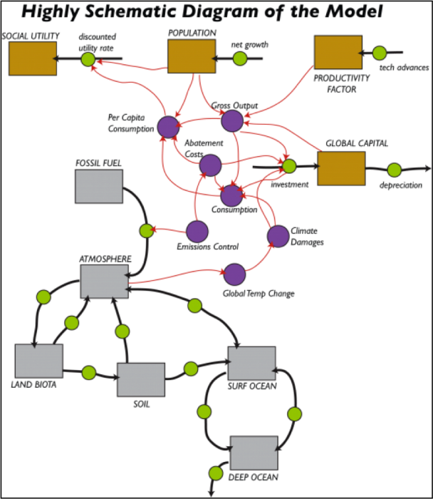
In this diagram, the gray boxes are reservoirs of carbon that represent in a very simple fashion the global carbon cycle model from Module 8; the black arrows with green circles in the middle are the flows between the reservoirs. The brown boxes are the reservoir components of the economic model, which include Global Capital, Productivity, Population, and something called Social Utility. The economic sector and the carbon sector are intertwined — the emission of fossil fuel carbon into the atmosphere is governed by the Emissions Control part of the economics model, and the global temperature change part of the carbon cycle model affects the economic sector via the Climate Damage costs. Let’s now have a look at the economic portions of the model. You should view this video about the DICE Economic Model [2] first, and then study the text that follows.
The Global Capital Reservoir
The Global Capital Reservoir
In this model, Global Capital is a reservoir that represents all the goods and services of the global economic system; so this is much more than just money in the bank. This reservoir increases as a function of investments and decreases due to depreciation. Depreciation means that value is lost as things age and the model assumes a 10% depreciation per year; the 10% value comes from observations of rates of depreciation across the global economy in the past. The investment part is calculated as follows:
Investment = Savings Rate x (GDP - Abatement Costs – Climate Damages)
The savings rate is 18.5% per year (again based on observations). The GDP is the total economic output for each year, which depends on the global population, a productivity factor, and Global Capital.
Abatement Costs
The Abatement Costs are the costs of reducing carbon emissions and are directly related to the amount by which we reduce carbon emissions. If we take steps to reduce our carbon emissions either by switching to renewable energy or improving efficiency or by direct removal of CO2 from the atmosphere, then there are costs associated with these steps. The model includes something called the abatement cost per GT C — this is the cost in trillions of dollars for each gigaton of carbon removed, and it can be changed over time. The default value is $3 trillion/GT C, which is a lot because it also includes the costs of large battery systems and new electrical transmission lines. But, the good thing about these costs is that once you pay for a GT of C removed, you don’t keep paying for it. If we were to completely cut all carbon emissions (currently around 10 GT C/yr) and do it in one year, it would cost $30 trillion or about 1/3 of the global GDP.
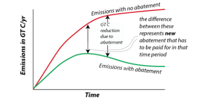
The diagram below shows how the abatement costs each year are figured out.
Climate Damages
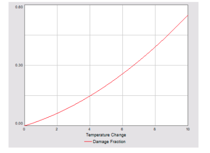
Climate Damages are the costs associated with rising global temperatures, including the costs of dealing with sea level change along coasts, extreme weather events (hurricanes, flooding, droughts, wildfires, etc.), labor (reduced productivity at higher temps), and increased human mortality (loss of workers hurts the economy). In the model, the climate damages are calculated as a fraction (think of this as a percentage) of the GDP. The fraction is a quadratic equation that looks like this:
damage fraction = slope × ΔT + coefficient × ΔTexponent
The ΔT is the global temperature change in °C. Both the slope and exponent can be adjusted in the model; the coefficient is set at 0.003. The default slope is 0.025 and the exponent is 2, which means that if we have a global temperature change of 4°C, damages equal to 15% of GDP; this rises to a devastating 55% for a temperature increase of 10°C. The diagram below shows what this damage fraction equation looks like, plotted as a function of temperature change in °C.
Relative Climate Costs
It will be useful to have a way of comparing the climate costs — the sum of the Abatement Costs and the Climate Damages — in a relative sense so that we see what the percentage of these costs is relative to the GDP of the economy. The model includes this relative measure of the climate costs (in trillions of dollars) as follows:
Relative Climate Costs = (Abatement Costs + Climate Damages) x GDP/initial GDP
Consumption
Consumption
Also related to the Global Capital reservoir is a converter called Consumption. A central premise of most economic models is that consumption is good and more consumption is great. This sounds shallow, but it makes more sense if you realize that consumption can mean more than just using things it up; in this context, it can mean spending money on goods and services, and since services include things like education, health care, infrastructure development, and basic research, you can see how more consumption of this kind can be equated with a better quality of life. So, perhaps it helps to think of consumption, or better, consumption per capita, as being one way to measure quality of life in the economic model, which provides a measure for the total value of consumed goods and services (in trillions of dollars), which is defined as follows:
Consumption = Gross Output – Climate Damages – Abatement Costs – Investment
This is essentially what remains of the GDP after accounting for the damages related to climate change, abatement costs, and investment.
The model also calculates the per capita consumption by just dividing the Consumption by the Population, and it also includes a converter called relative per capita consumption, which is just the per capita consumption divided by the GDP. In the model, this is in thousands of dollars per person.
Population & Productivity Factor
Population & Productivity Factor
Population
The population in this model is highly constrained — it is not free to vary according to other parameters in the model. Instead, it starts at 6.5 billion people in the year 2000 and grows according to a net growth rate that steadily declines until it reaches 12 billion, at which point the population stabilizes. The declining rate of growth means that as time goes on, the rate of growth decreases, so we approach 12 billion very gradually.
Productivity Factor
The model assumes that our economic productivity will increase due to technological improvements, but the rate of increase will decrease (but will not go negative), just like the rate of population growth. So the productivity keeps increasing, but it does not accelerate, which would lead to exponential growth in productivity. This decline in the rate of technological advances is once again something that is based on observations from the past.
Emissions
Emissions
The model calculates the carbon emissions as a function of the GDP of the global economy and two adjustable parameters, one of which (carbon intensity) sets the emissions per dollar value of the GDP (units are in gigatons of carbon per trillion dollars of GDP) and something called the Emissions Control Rate (ECR). The equation is simply:
Emissions = carbon intensity*(1 -ECR)*GDP ;
Currently, carbon intensity has a value of about 0.118, and the model assumes that this will decrease as time goes on due to improvements in the efficiency of our economy — we will use less carbon to generate a dollar’s worth of goods and services in the future, reflecting what has happened in the recent past. The ECR can vary from 0 to 1, with 0 reflecting a policy of doing nothing with respect to reducing emissions, and 1 reflecting a policy where we do the maximum possible. Note that when ECR = 1, then the whole Emissions equation above gives a result of 0 — that is, no human emissions of carbon to the atmosphere from the burning of fossil fuels. In our model, the ECR is initially set to 0.005, but it can be altered as a graphical function of time to represent different policy scenarios. In other words, by changing this graph, we are effectively making a policy — and everyone follows this policy in our model world!
Making Comparisons — the Discount Rate
Making Comparisons — the Discount Rate
We would like to be able to see whether one policy for reducing emissions of carbon is economically better than another. Different policies will call for different histories of reductions, and to compare them, we need to find a way to compare the expected future damages associated with each policy. A problem comes when we try to compare 200 million in damages at some time in the future vs. 20 million in damages today. Economists use something called a discount rate to do this. Here is an example to help you see how this idea works: imagine you have a pig farm with 100 pigs, and the pigs increase at 5% per year by natural means. If you do nothing but sit back and watch the pigs do their thing, you’d have 105 pigs next year. So 105 pigs next year can be equated to 100 pigs in the present, with a 5% discount rate. Thus, the discount rate is kind of like the return on investment. Now think about climate damages. If we assume that there is a 4% discount rate, then $1092 million in damages 100 years from now is $20 million in present-day terms. Here is how this works in an equation:This is a standard exponential growth equation is called Euler’s number and has a value of about 2.7. Now, let’s say we calculate some cost in the future — 8 million dollars 200 years from now — we can apply a discount rate to this future cost in order to put it into today’s context. Here is how that would look:
It is important to remember that this assumes our global economy will grow at a 4% annual rate for the next 200 years. The 4% figure is the estimated long-term market return on capital, but this may very well grow smaller in the future, as it does in our model. Although we’re not going to dwell on the discount rate any more in this exercise, it is good to understand the basic concept.
A simpler way of comparing future costs or benefits with respect to the present is to express these costs and benefits relative to the size of the economy at any one time — which our model will calculate. This gets around the kind of shaky assumption that the economy is going to grow at some fixed rate. These relative economic measures are easy to do — just divide some parameter from the model, like the per capita consumption, by the GDP. Below is a list of the model parameters that we will keep an eye on in the following experiments:
Below is a list of the model parameters that we will keep an eye on in the following experiments:
Global capital — the size of the global economy in trillions of dollars;
GDP — the yearly global economic production in trillions of dollars
Per capita consumption — consumption/population; this is a good indicator of the quality of life — the higher it is, the better off we all are; units are in thousands of dollars per person
Relative per capita consumption — annual per capita consumption x (GDP/initial GDP); again, a good indicator of the quality of life, in a form that enables comparison across different times; units are in thousands of starting time dollars per person
Sum of relative pc consumption — the sum of the above— kind of like the final grade on quality of life. If you take the ending sum and divide by 200 yrs, it gives the average per capita consumption for the whole period of the model run.
Relative climate costs — an annual measure of (abatement costs + climate damages) x (GDP/initial GDP); this combines the costs of reducing emissions with the climate damages, in a form that can be compared across different times; the units are trillions of dollars.
Sum of relative climate costs — sum of the relative climate costs — the final grade on costs related to dealing with emissions reductions (abatement) and climate; this is the sum of a bunch of fractions, so it is still dimensionless.
Global temp change — in °C, from the climate model
Experiment 1
Experiment 1 - Changing the Emissions Control Rate (ECR)
In the model [3], the ECR can vary from 0 to 1, and it expresses the degree to which we take steps to curb emissions; a value of 0 means we do nothing, while a value of 1 means that we essentially bring carbon emissions to a halt. According to Nordhaus, the most efficient way of implementing this control is through some kind of carbon tax, in which case a value close to 1 represents a very hefty carbon tax that would provide strong incentives to develop other forms of energy. In this experiment, we’ll explore 3 scenarios — in A, we’ll keep ECR at a very low level — this is the “do nothing” policy scenario, in B we'll ramp it up steadily through time — this is the “slow and steady” policy scenario, and in C, we’ll ramp it much more quickly, eventually reaching a value of 1.0 — this is the “get serious” policy scenario. You can make these changes in the ECR by altering the graphical converter.
The three different scenarios consist of 5 numbers that are the ECR values for 5 points in time (corresponding to the five vertical lines in the graph); these times are the years 2000, 2050, 2100, 2150, and 2200. There are 2 videos to watch in Module 10 Summative Assessment— the Model Introduction, which gives you an overview of the model and ECR Scenarios which explains how to modify the model to do these problems.
| 1. Do nothing | 2. Slow and Steady | 3. Get Serious | |
|---|---|---|---|
| Practice | Use defaults values (no need to change anything) | 0.005; 0.15; 0.3; 0.45; 0.6 (see video about adjusting these) |
0.005; 0.33; .66; 1.0; 1.0 |
| Graded | Use defaults values (no need to change anything) | 0.005; 0.2; 0.4; 0.6; 0.8 | 0.005; 0.5; 1.0; 1.0;1.0 |
For each scenario, run the model, study the model results, and record the results indicated in the table below and then refer to your results in answering the questions below.
This short video below explains how to make changes to the model. Please take a few minutes to watch the ECR Scenarios video. You will be happy you did later!
Video: ECR Scenarios (5:45)
For this summative assessment, we're basically going to do three different runs with this model. Each one will have a different history of the emissions control rate. So when you open the model up, just reset everything first. The reset button clears everything. Then we're gonna run it with the default values. So for the practice version we use the default values, we're not gonna change anything, we're just gonna run it. We run it and see what happens. Here you can see in red the temperature rising and it gets up to about six point eight degrees Celsius warming. In blue is the carbon emissions that rises and it reaches a peak of about thirty-one gigatonnes of carbon. And then it starts to decrease and then it just sort of ;falls off a cliff right here. It falls off a cliff right there because we actually would run out of fossil fuels at that point. And if you click ahead a few graphs, you can see...there's the emissions. Sorry, go back one. This graph shows the fossil fuels remaining. That drops to zero at this point, so we've totally run out of fossil fuels at that point. So that's a scenario number one. That's they do-nothing scenario.
The next scenario B is called the slow and steady one. And if you look over here in this table, there are some numbers that tell us the values of this emissions control rate at different points in time. So here's what you do. You click on the emissions control right here. You click on table and then these Y values here, ;the numbers that are reflected over here. So .005 point is already there. Now we're gonna put in 0.15, and then 0.3, and then 0.45, and then finally 0.60, and hit okay. And now we see we have a nice slow steady increase in the emissions control rate. That means as time goes on we're gonna kind of slowly do more and more in terms of reducing carbon emissions. That's all we have to change and then we run the model and you see that that results in a somewhat lower global temperature change. Still rises to 5.45 degrees C which is a pretty serious warming by the year 2200.
Now, will it will do one more scenario. This is the get-serious scenario and the values here according to the table are .33, .66, and then 1.0. Now when this has a value one, that effectively means we're going all out, we're going to do whatever it takes to eliminate all carbon emissions. And so we set that up and you can see here it tops out and stays at one there. We run that scenario and sure enough the temperature changes quite a bit less. We have 2.8 degrees of temperature change by the end of time. And you know if you look at the carbon emissions, let's see if you go to this one here, this is all three runs carbon emissions. So the third one would get serious. The carbon emissions they actually drop to zero by the time we get to the year 2152. And they stay at zero at that point.
So then, you've done these three runs. On a number of these graphs, the different curves are presented...run one, run two, run three. So run one would be the do-nothing scenario, run two would be the slow and steady scenario, and run three would be the get-serious scenario. And so there are a whole bunch of different graphs here. Everything is plotted. Here, by the way, these are the total abatement costs. And you can see in the first run the abatement costs are essentially zero all the way along. And then the abatement costs get very big once we've run out of fossil fuels. We have to make up for that with renewable energy and so that's going to be associated with some significant cost. The abatement costs rise up dramatically there and then level off as time goes on.
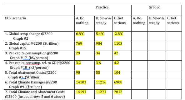
So then, in this worksheet, you see there are a whole bunch of questions to answer. What is the global temperature change at the year 2200 for a scenario A, ;B, and C? And these are the answers that you could get off of these graphs. Graph number 2, graph number 15, 17, 18, 7, 9, and so on. from doing these three scenarios and then toggling back and forth between these graphs, running your cursor along here until you get to the year 2200, and then recording the values, and filling them in in this table. So, if you fill in this part of the table with those values, then you can use these numbers to help you answer the various questions that go along with this experiment.
If you haven't already run the model for this experiment, run the Model now! [4]
For each scenario, study the model results, and record the results indicated in the table below and then refer to your results in answering the questions below.
| Items | Do nothing | Slow and Steady | Get Serious |
|---|---|---|---|
| 1. Global temp change @ 2200 | |||
| 2. Global capital @ 2200 | |||
| 3. Per capita consumption @ 2200 | |||
| 4. Relative per capita consumption @ 2200 | |||
| 5. Sum of relative per capita consumption @ 2200 | |||
| 6. Relative climate costs @ 2200 | |||
| 7. Sum of relative climate costs @ 2200 |
Questions
1. Which of these 3 scenarios leads to the lowest global temperature change?
- Do nothing
- Slow and steady
- Get serious
2. For answer to #1, global temp change @2200 = ____________ (±0.5°C)
3. Which of these 3 scenarios leads to the highest global capital?
- Do nothing
- Slow and steady
- Get serious
4. For answer to #2, global capital @2200 = ____________ (trillion$ ±50)
5. Which of these 3 scenarios leads to the lowest relative climate costs?
- Do nothing
- Slow and steady
- Get serious
6. For answer to #5, relative climate costs @2200 = _______________ (±0.5)
7. Which of these 3 scenarios leads to the greatest relative per capita consumption?
- Do nothing
- Slow and steady
- Get serious
8. In terms of both economic costs (lowest relative climate costs) and benefits (highest relative per capita consumption), which scenario is the best?
- Do nothing — best in both costs and benefits
- Slow and steady — best in both costs and benefits
- Get serious — best in both costs and benefits
- Do nothing — best in benefits; Get serious — best in costs
- Slow and steady — best in benefits; Do nothing — best in costs
Now we step back and consider what we’ve done and learned by responding to the following questions.
9. You have probably heard people (mainly from the realms of business and politics) say that we should not do anything about global climate change because it is too expensive and will hurt our economy. After experimenting with this model, do you agree with them, or do you think they are missing something (and if so, what is it they are missing)?
10. Remember that each ECR history reflects a different economic/political policy. Briefly explain how you came to figure out which policy was the best. In answering this, you have to think about what “best” means — the least environmental damage; the greatest economic gain per person; the easiest policy to implement; or some combination of these?