Module 6: Groundwater Hydrology
Module 6: Groundwater Hydrology
Overview
In this two-part module, we will focus on the occurrence and movement of groundwater. Key topics will include an overview of aquifer types and nomenclature, and the physical properties and processes that govern the storage, transport, rate of flow, and budgets of water in these systems. In addition, we will examine some examples of large-scale aquifer systems in the U.S., including those underlying the Valley & Ridge province and in the semi-arid American West. The module has two parts and is designed as a two-week course. The first section (Module 6.1) focuses on aquifers and their properties, with a series of case studies that outline the geometry and geology of highly-used regional aquifers. The second section (Module 6.2) focuses on the dynamics of aquifers, including the driving forces for water movement, flow rates, flow to pumping wells, and water budgets.
6.1 Aquifers and Properties
6.1 Aquifers and Properties
In the first part of this module, we will focus on the properties of aquifers: What characteristics of a rock or sediment make it a good aquifer? What are the different kinds of aquifers? Fundamentally, the ability to store and transmit water are the two key ingredients that make a subsurface geological formation useful as an aquifer. In Module 6.1, we will explore the detailed physical properties of rocks and sediments that ultimately affect the storage and movement of groundwater. We'll also illustrate with a series of well-known examples of large aquifers tapped for drinking, industrial, and agricultural uses.
Goals and Objectives
Goals and Objectives
Goals
- Explain the distribution and dynamics of water at the surface and in the subsurface of the Earth
- Interpret graphical representations of scientific data
Learning Objectives
In completing this lesson, you will:
- Identify the properties of artesian wells and describe the conditions under which they form
- Explain the difference between porosity and permeability
- List and describe the properties of aquifers that control the movement and storage of groundwater
- Explain the role of fractures in determining the transmission properties of aquifers
- Use Darcy's Law to explain the roles of aquifer properties and driving forces in governing the rate of groundwater flow
Aquifers Explained
Aquifers Explained
Aquifers come in many shapes, sizes, and “flavors”. For example, some aquifer systems span hundreds – or even thousands – of kilometers across several states or nations and may include multiple individual layers of rock or sediment that total thousands of meters in thickness. Other aquifers may be restricted to a few kilometers within a stream valley, and be only a few meters thick.
Nonetheless, there are some important common features of different kinds of aquifers. In this section of the module, we provide a basic overview of aquifers: What is an aquifer? What are the different types of aquifers, and what is their anatomy?
Overview and Nomenclature
Overview and Nomenclature
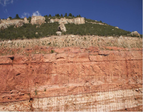
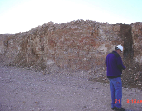
Aquifers are geologic formations in the subsurface that can store & transmit water (Figures 1 and 2). As we will see later in the section titles Basic Aquifer Properties, there are specific rock and soil properties that govern these two functions. Adequate storage requires that there be sufficient void space between particles, in fractures, or generated by compressing the aquifer under pressure, to provide usable quantities of water. Adequate transmission requires that the void spaces where water occurs be well enough connected that it can percolate or flow under either natural or pumping-driven conditions, at a rate that will support sustained use.
These definitions are intentionally vague because they depend on the scale of intended use. For example, an aquifer that provides water for a large city will need to sustain higher pumping rates at wells (on order of tens of thousands of gallons per minute) than one that provides for a single-family (a few to perhaps ten gallons per minute). For reference, Penn State University relies almost exclusively on groundwater pumping for its water supply at the University Park campus, with a total extraction of ~2.5 million gallons per day (about 1750 gallons per minute) distributed among several pumping well fields.
In contrast to an aquifer, an aquitard, often also termed a confining layer or aquiclude, is a geologic formation in the subsurface that does not transmit water effectively – and therefore acts as a barrier to groundwater flow. In general, aquifers are usually composed of sediments or sedimentary rocks with grain sizes larger than fine- to medium sand (>~125 µm diameter), or of fractured rock. Aquitards are typically composed of fine-grained sediments or sedimentary rocks or those in which the pore spaces have been filled by mineral cements (silts, siltstones, shales, clays, cemented sandstones, or unfractured limestones).
Aquifer Anatomy
Aquifer Anatomy
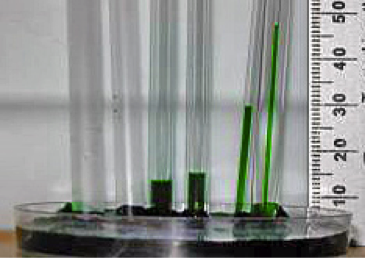
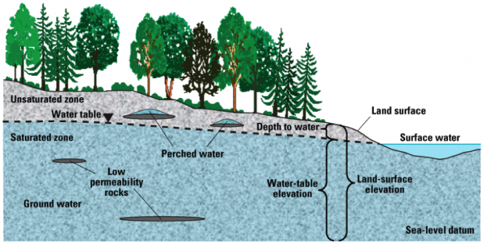
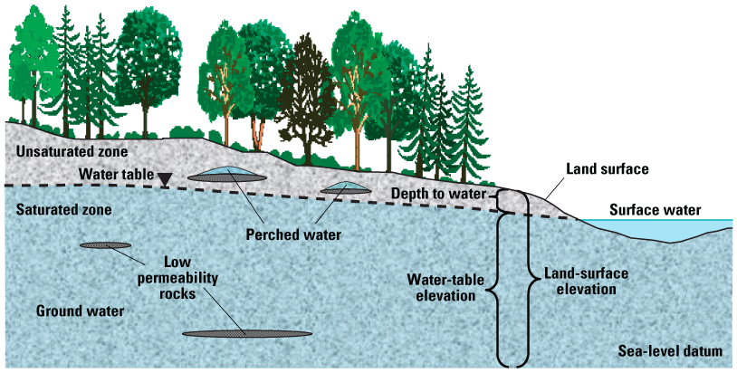
In the simplest sense, you might imagine an aquifer formation that may be covered by a veneer of soil, and which extends downward from a few feet below the surface for several tens or even hundreds of feet (Figure 3). At some depth below the land surface, the interstices between soil or sediment particles, or the fractures in the rock, will be water-filled or saturated. Shallower than that depth, these interstices, or pore spaces, will be filled with air, water vapor, and some liquid water bound to the surfaces of the rock (Figures 3-5). This zone is the unsaturated zone, also known as the “zone of soil moisture” or the vadose zone. The water table marks the top of the ground water system and is formally defined as the depth at which the pressure in the subsurface is equal to the atmospheric pressure. Immediately above the water table, there is a narrow zone of saturation termed the capillary fringe. In this zone, water is wicked upward in pore spaces due to capillary forces. This is analogous to capillary tube experiments you may have seen or performed in physics or chemistry classes in high school; it occurs due to interaction between the polar water molecule and the surfaces of the solids, and is directly related to the fact that water has a surface tension (as you may remember from Module 1!). In the capillary fringe, pores are saturated, but pressures are sub-atmospheric, meaning that the water is under suction as it is pulled or wicked upward. The nomenclature “fringe” reflects the fact that slight variations in grain size lead to variations in the height that water is drawn (again, think to the capillary tube experiment, and effects of different tube sizes) (Figure 5).
Any precipitation or surface water that infiltrates to the water table must percolate through the vadose zone in order to recharge the aquifer. As we will see later in this module infiltration and recharge typically constitute only a small fraction – rarely more than 10% - of precipitation, because most water that falls in events is returned to the atmosphere by transpiration or evaporation, becomes runoff (i.e., if the capacity for infiltration is exceeded by the rate of precipitation), or is bound by soils in the vadose zone.
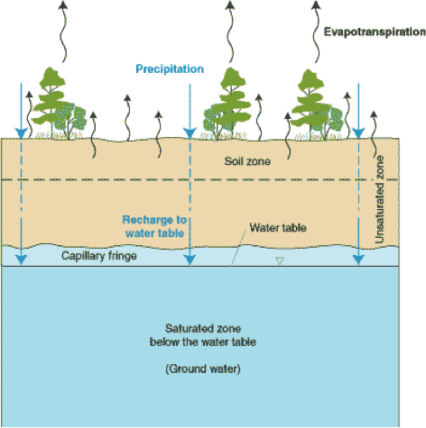
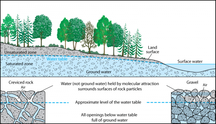
Water (not ground water) held by molecular attraction surrounds surfaces of rock particles. All openings below the water table are full of ground water. The Unsaturated Zone is on the land surface and above the water table which contains the saturated zone, surface water, and ground water.
Types of Aquifers
Types of Aquifers
In more detail, there are three main classifications of aquifers, defined by their geometry and relationship to topography and the subsurface geology (Figures 6-9). The simple aquifer shown in Figure 6 is termed an unconfined aquifer because the aquifer formation extends essentially to the land surface. As a result, the aquifer is in pressure communication with the atmosphere. Unconfined aquifers are also known as water table aquifers because the water table marks the top of the groundwater system.
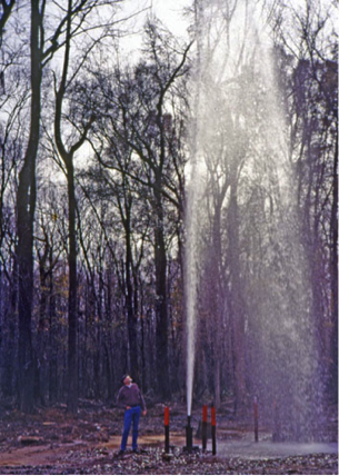
A second common type of aquifer is a confined aquifer, which is isolated from pressure communication with overlying or underlying geologic formations – and with the land surface and atmosphere – by one or more confining layers or confining units. Confined aquifers differ from unconfined aquifers in two fundamental and important ways. First, confined aquifers are typically under considerable pressure, which may be derived from recharge at a higher elevation or from the weight of the overlying rock and soil (known as the overburden). In some cases, the pressure is high enough that wells drilled into the aquifer are free-flowing. This condition requires that the water pressure in the aquifer is sufficient to drive water up the wellbore and above the land surface, and such wells are called artesian wells (Figure 7). Second, confined aquifers typically remain saturated over their entire thickness, even as water is removed by pumping wells. Water extracted from the aquifer comes only from the depressurization of the aquifer – a combination of depressurization and expansion of the water itself, and relaxation of the aquifer formation upon reduction in pressure (Figure 8).
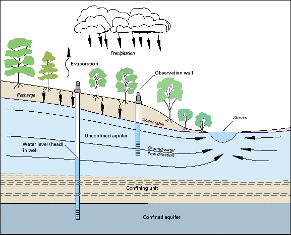
The third main type of aquifer is a perched aquifer (Figure 6). Perched aquifers occur above discontinuous aquitards, which allow groundwater to “mound” above them. Thee aquifers are perched, in that they sit above the regional water table, and within the regional vadose zone (i.e. there is an unsaturated zone below the perched aquifer). The dimensions of perched aquifers are typically small (dictated by climate conditions and the size of aquitard layers), and the volume of water they contain is sensitive to climate conditions and therefore highly variable in time.
Aquifer Properties
Aquifer Properties
In the previous section, you’ve learned about the different types of aquifers, and the basic characteristics that define an aquifer – namely the ability to store and transmit water. But what, exactly, about a rock or sediment beneath the ground determines whether the rock can hold water, or whether water can percolate through it? In the following section, we will explore this question in more detail, to define the important individual properties of the rock.
Storage
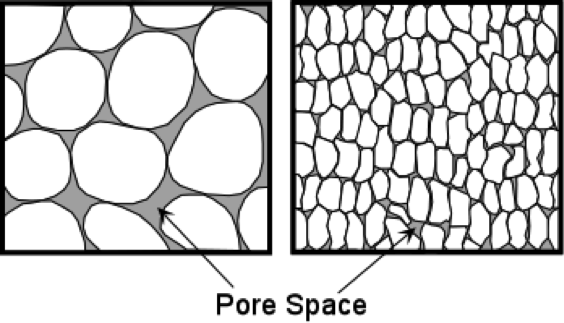
Porosity (usually denoted by the symbol η, which is Greek letter 'eta') is the primary aquifer property that controls water storage, and is defined as the volume of void space (i.e., that can hold water in the zone of saturation) as a proportion of the total volume (Figure 10).
Porosity is expressed as either a fraction, or a percentage:
, or if reported as a percentage,
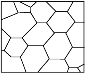
For aquifers composed of sedimentary rocks or sediments, porosity is usually in the range of ~10-35%. For unfractured crystalline rock, porosity is quite a bit lower - on order of a few percent - because there is little porosity between individual grains other than the vary narrow interfaces along their boundaries (Figure 10).
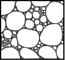
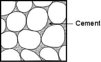
Several factors can affect porosity. In sedimentary rock and sediments, controls on porosity include sorting, cementation, overburden stress (related to burial depth), and grain shape. Poorly sorted sedimentary deposits, in which there is a wide distribution of grain sizes, typically have lower porosity than well-sorted ones (Figure 11). This is because the finer particles are able to fill in spaces between the larger grains. Cementation caused by precipitation of minerals (typically calcium carbonate or silica) at grain boundaries also reduces porosity (Figure 11). Angular grains generally allow more efficient packing of particles than rounded or spherical ones, also leading to slightly lower porosity. Finally, the more deeply sediments or sedimentary rock are buried, the larger the weight of the overburden; the higher stress leads to compaction, tighter packing of the grains, and lower overall porosity.
Secondary processes that act on the rock or sediment after its formation, primarily weathering by physical or chemical mechanisms, can also affect porosity. Physical weathering by wind or water movement can remove fine clay-sized particles from the sediment (a process termed winnowing), leading to increased porosity near the Earth’s surface. Chemical weathering of certain rock types can lead to clay and oxide formation; depending on the environment and initial composition of the aquifer grains, the clays and oxides may subsequently be removed (porosity increase), or they may grow at the boundaries of other particles and reduce the porosity.
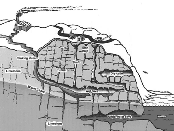
In fractured rock (whether fractured crystalline or cemented sedimentary rock), porosity is typically ~2-5%. The pore space is almost entirely composed of the fractures or cracks themselves, which are typically a millimeter or less in aperture (Figure 12). Two primary factors control porosity – and the connectedness of porosity – in fractured rock. First, increased stress, related to the depth of burial and the weight of the overburden, exerts a clamping force that causes the closure of cracks or fractures (decreases fracture aperture). In some types of rock – most notably limestones – chemical weathering occurs via dissolution as water flows along and through fractures. This leads to increased fracture aperture. Significant enlargement of fractures can lead to the development of karst, typified by large open fractures, caves, and caverns, as well as sinkholes and hummocky topography that ensue as the underlying rock is gradually dissolved (Figure 13).
Interestingly, grain size does not affect porosity. For example, consider a box filled with spherical particles packed as tightly as possible. The proportion of empty space (porosity) would be the same whether the particles are marble-sized, pea-sized, or golf ball-sized; the porosity is controlled entirely by the geometry of the particles – not their dimensions. As we’ll see in the next section, however, grain size does strongly affect the ability of aquifers to transmit water because it directly controls the size of the pore spaces where the water percolates. For example, unconsolidated clays (grain sizes of a few to tens of microns) commonly have porosities of over 50-60%, but they transmit water only one-thousandth to one millionth as well as sands with porosities of 20-30% (grain sizes of a few hundred microns).
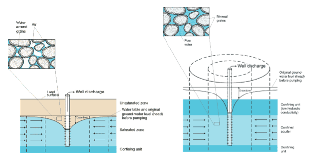
Specific Yield (denoted as Sy) is another important quantity for water storage in unconfined aquifers. Sy is defined as the proportion of water occupying void spaces that drains under gravity. Because some water is bound, or adsorbed, to the aquifer particles or fractures, the specific yield is always lower than the porosity (take a look at Figure 8 [7], inset at top left). The attraction between water molecules and the aquifer is due – you guessed it! – to the polar nature of water and surface tension. In sands and fractured rock, Sy is typically a large fraction (>90%) of the porosity, whereas in fine-grained sedimentary deposits Sy may be as low as a few percent because the surface area interacting with water molecules is higher, and pores are smaller, allowing the aquifer to retain more water. In unconfined aquifers, Sy controls the amount of water that can be extracted by pumping.
In confined aquifers, the compressibility of the aquifer is the dominant control on water storage and release. As described above (see Figure 8, right panel), when water is extracted from confined aquifers by pumping or flow to natural springs, the aquifer remains saturated, but the water pressure decreases. Upon depressurization, the aquifer itself can compress slightly. If water is recharged or injected, the opposite occurs: pressure increases and the aquifer expands very slightly. Essentially, by increasing water pressure, more water mass is being “crammed” into the pore space in the aquifer, and vice versa. Although exaggerated, one way to visualize this is to think of pores in the rock or aquifer as a juice box. By changing the pressure inside the box, it will expand or contract. In the same way that a soft juice box will deform more than a stiff one for a given change in pressure, a more compressible aquifer will yield more water than a stiffer aquifer, for the same depressurization. The storage of water in confined aquifers is termed the specific storage, and reported in units of Volume of water/Volume of aquifer per change in water level (so the units are 1/length; e.g., 1/m or 1/ft).
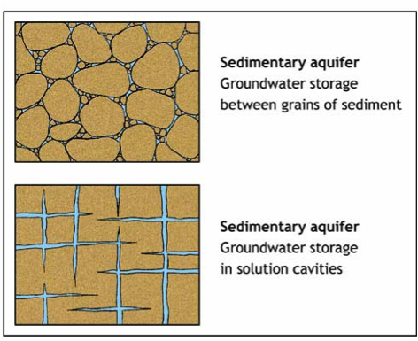
Sedimentary aquifers with intergranular porosity have groundwater storage between grains of sediment. Sedimentary aquifers with fracture porosity have groundwater storage in solution cavities.
Transmission
Transmission
The ability of an aquifer to transmit water – or of an aquitard to slow the flow of water – is the second essential ingredient controlling groundwater movement. It is also the most variable in natural materials; distances in astronomy are the only other quantity in nature that varies over a similar range! For example, the difference in groundwater flow rate for shale vs. gravel is a factor of 1,000,000,000,000 (yup…one trillion). That’s the difference between the size of an iPhone and the distance from the Earth to the Sun.
Groundwater transport properties are described by two related quantities. Hydraulic Conductivity, denoted by K, is a measure of the ability of a particular fluid (usually water) to flow through the rock or sediment. Permeability, denoted by a lower-case k, is often also termed “intrinsic permeability” and describes the ability of the geologic formation alone to transmit fluid. Although related, the key difference is that hydraulic conductivity combines properties of the geologic formation and the fluid, whereas permeability describes only the rock properties. As described in Sidebar 1, the basic concept of hydraulic conductivity emerged from a series of ingenious experiments conducted in the mid-1880s by Henri Darcy, a French Engineer. These experiments led to Darcy’s Law, which forms the foundation for much of modern hydrogeology and petroleum engineering.
To illustrate the difference between K and k, consider the sandstone in Figure 14 below. The sandstone itself has a permeability, which is controlled by the size of the grains and pore spaces through which water can percolate, and the connectedness and geometry of the pores (more on that in a moment!). That permeability is a characteristic of the sandstone, regardless of whatever fluid might be moving through it, the temperature, or anything else. But the flow rate of water through this sandstone will be different than for oil, or for air, or any other fluid. So the same sandstone also has a hydraulic conductivity specific to a given fluid of interest.
Viscosity and Density
Viscosity and Density
More specifically, it is the viscosity and density of the fluid that matter. More viscous fluids will flow more slowly through the same rock than less viscous ones. This is important for comparing different fluids (say, oil vs. water – whether you are thinking about an oil reservoir or contamination of groundwater by a gasoline spill). It is also important in considering the effects of temperature, because water viscosity decreases with increasing temperature: it’s less than half as viscous at 90° than at 32° F. So even for the same aquifer, the hydraulic conductivity goes up if it is warmer! This makes some sense – if the water is less viscous (i.e. “thinner”), it will flow more easily through the aquifer.
So…that’s how we define permeability and hydraulic conductivity. But what controls their magnitude? The main factors are grain size and shape, sorting, porosity (degree of compaction or fracture aperture), particle orientation or alignment that affects the tortuosity of the flow path, and cementation. Tortuosity is a measure of how far fluid must go to “circumnavigate” its way around particles: higher tortuosity indicates that water must go farther to get to its destination (a more tortuous path). For all of these mechanisms, the key underlying control on groundwater movement is the viscous resistance resulting from the interaction of the fluid with solid surfaces in the aquifer (grain edges or fracture walls).
Importance of Fractures
Importance of Fractures
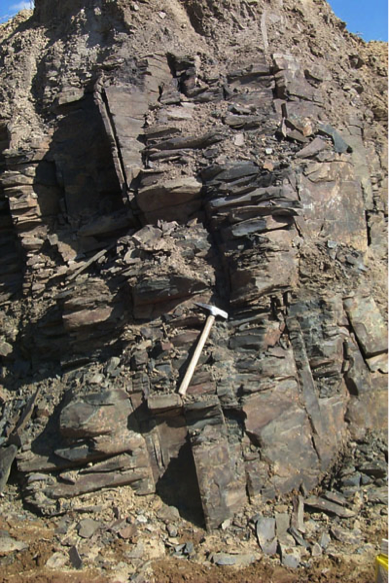
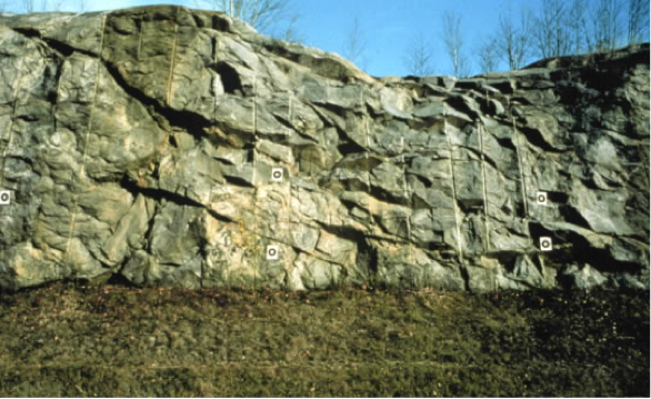
Fractured aquifers are one important and widely used class of aquifer because they are commonly both highly permeable and rapidly recharged. For example, groundwater recharge to the limestone aquifer beneath Nittany Valley in the Spring Creek watershed is around 30-45% of the annual precipitation (in comparison to typical recharge of <10% of precipitation). Fractured aquifers are permeable despite their overall low porosity (usually <5%) because natural fractures usually form in consistent orientations and are well connected in networks over hundreds of meters to tens of kilometers or more (Figures 15-16). The preferred orientation of major fractures leads to anisotropy in permeability, in which the aquifer may be more permeable parallel to the dominant fracture directions than in other orientations.
The rapid flow rates and direct pathways for recharge from the land surface also lead to concerns specific to fractured aquifers. In the absence of confining layers or thick soils, rapid recharge along fractures that extend to or nearly to the land surface increase vulnerability of contamination by surface activity, including fertilization of fields, pesticide application, or spills. Direct connections between surface water bodies and groundwater through major fracture systems also increase the potential for water-borne pathogens to enter the groundwater system, especially during periods of high flow or if confining layers along stream beds are breached. Compounding this risk, if contamination does occur, flow along fracture networks can be very rapid and the direction and rates of contaminant transport difficult to predict - unless the fracture network in the subsurface is extraordinarily well known, which is rarely the case. Because of their potential for contamination, fractured aquifers are a subject of highly active research, including dedicated large-scale field programs (e.g., check out the U.S. Geological Survey’s Mirror Lake project [9]).
Regional Aquifer Systems: Examples
Regional Aquifer Systems: Examples
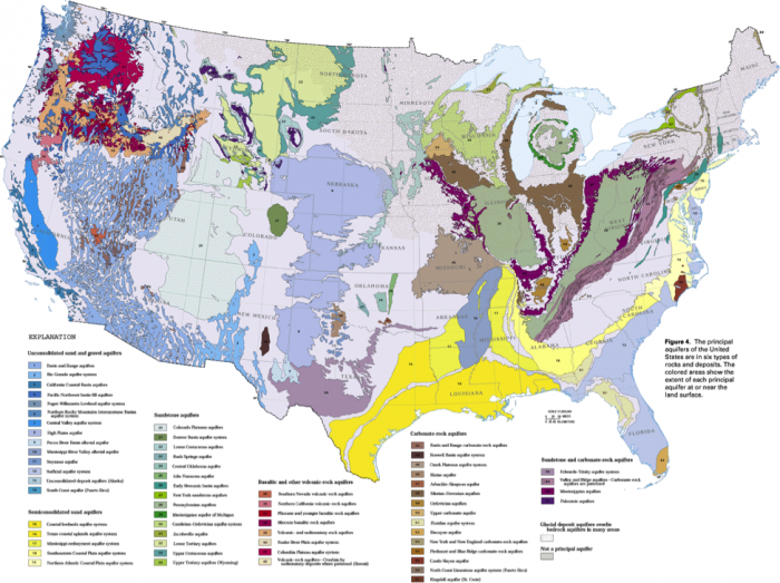
Ground water flow systems extend over a wide range of scales, from small perched aquifers that may supply water for a single-family, to regional rock formations that span thousands of km and cross several states (Figure 18). These regional systems supply water for irrigation and domestic uses in many areas, especially in semi-arid and arid parts of the American West and coastal population centers along the East coast (remember Module 1, figures 10-12?). These regional systems commonly consist of several layered sedimentary formations and may extend to several kilometers in depth. The U.S. Geological Survey has compiled detailed studies of regional aquifer systems across the U.S., with useful information about climate, recharge, subsurface geology, use, and problems related to water quality or quantity (a list and links for each of the principal regional aquifers in the U.S can be found at USGS Groundwater Information [11]. A detailed atlas with information about the major aquifer systems in particular regions of the U.S. can be viewed at USGS Ground Water Atlas of the United States [12]. In this module, we will focus on a few example regional aquifer systems of particular relevance to the Northeastern and mid-Atlantic U.S. and the Central Valley of CA.
Valley and Ridge Aquifer System
Valley and Ridge Aquifer System
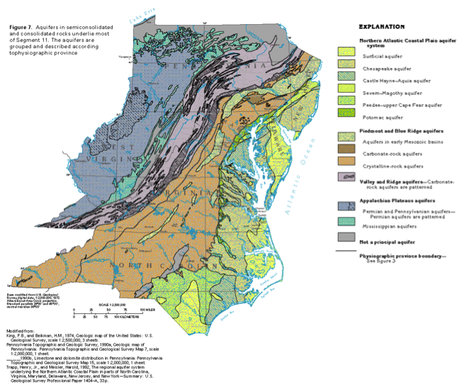
The Valley and Ridge aquifer system extends SW-NE across Central PA, West VA, and VA (Figure 19, purple area), and is the main water supply for much of this region. It is composed of layered Paleozoic sedimentary strata (shales, sandstones, and limestones) that were folded and deformed by a series tectonic collisions over 200 million years ago. The modern valleys in the Valley and Ridge province have formed where limestone, which is most susceptible to erosion, was exposed in the core of anticlines, or upfolds (Figure 20). The more resistant sandstones and shales form the regional ridges, like Mt. Nittany and Bald Eagle Ridge.
The principal aquifer unit in this system is the fractured limestone that underlies the valleys. As noted above, because it is fractured, it recharges rapidly, has a high fracture permeability, and wells drilled along the fractures are highly productive (c.f. Figure 17). Recharge is focused on the flanks of the ridges, where runoff flows over the less permeable shale and sandstone units and enters the groundwater through fractures or sinkholes above the limestone at the valley edges. Groundwater flow is generally toward the center of the valleys, and springs commonly feed the surface water systems. The water is characterized by a high hardness (Mg and Ca content; we’ll cover this in more detail in Module 7), derived from limestone dissolution. Dissolution of the limestone has formed extensive karst features (caves, caverns, sinkholes) throughout the region.
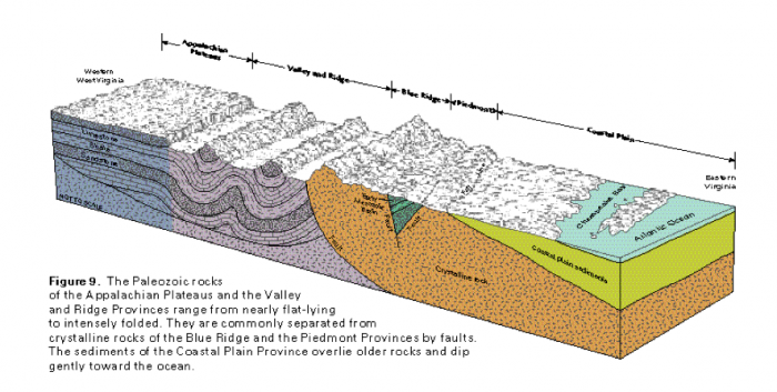
The Paleozoic rocks of the Appalachian Plateaus and the Valley and Ridge Provinces range from nearly flat-lying to intensely folded They are commonly separated from crystalline rocks of the Blue Ridge and the Piedmont Provinces by faults. The sediments of the Coastal Plain Province overlie older rocks and dip gently toward the ocean.
Atlantic Coastal Plain Aquifer System
Atlantic Coastal Plain Aquifer System
The Atlantic Coastal Plain aquifer system extends North-South along much of the Eastern portions of New Jersey, Delaware, Pennsylvania, Virginia, and North Carolina (Figure 19). It consists of a sequence of layered sedimentary aquifers (sands and gravels) separated by series of aquitards, all deposited starting around 100 million years ago and continuing today. The layers slope, or dip, to the East and extend offshore for tens of km beneath the continental shelf (Figure 21).
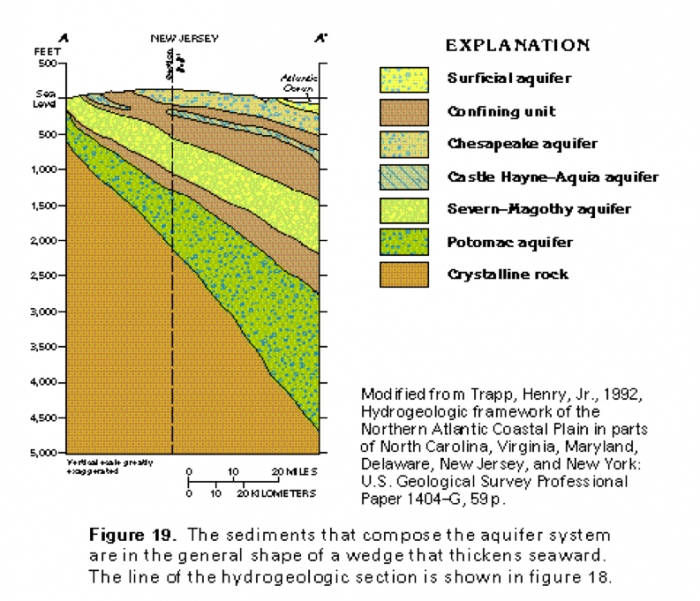
Recharge occurs by both natural and managed infiltration on land across much of the coastal plain; groundwater flow in the subsurface is mainly to the East along the sediment layers. One interesting consequence of this flow pattern is that there may be a sizable freshwater resource offshore that could be accessed by drilling in relatively shallow water on the continental shelf. During the last ice age, when conditions were substantially wetter than today and a nearly mile-thick ice sheet covered the northern extent of the aquifer system, recharge was probably even larger - and thus may have forced fresh water several tens of km offshore, where that “fossil” water may remain today!
The Atlantic Coastal Plain system is an important water source for domestic/municipal supply and industry in population centers throughout coastal North Carolina, Maryland, Virginia, Delaware, and New Jersey. However, concentrated, localized pumping has led to a reversal of flow direction (toward the wells instead of Eastward) in some of the aquifer units throughout the region. In addition to overarching concerns about the sustainability of withdrawals that exceed recharge rates, the flow reversal has led to local salt-water intrusion, whereby saline ocean water infiltrates the aquifer and in some cases renders it non-potable.
Central Valley/San Joaquin Valley Aquifer System
Central Valley/San Joaquin Valley Aquifer System
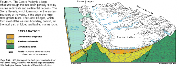
The Central Valley Aquifer system of Central CA lies in a large structural basin running approximately North-South, between the Coast Ranges to the West and the Sierra Nevada mountains to the East (Figure 22). The deep elongate basin is infilled with marine and continental sediments, primarily composed of interlayered sands and clays. The basin itself is formed by tectonic processes caused by East-West extension (these are the same forces that are causing continued uplift of the major mountain chains throughout the Basin and Range province of the Southwestern US, and which are one major control on orographic precipitation patterns in that region).
The continental deposits (Figure 22, orange) comprise the main aquifer units and range from one-half to over two miles in thickness. As is the case in the Valley and Ridge, the recharge is primarily focused around the valley perimeter as runoff over the flanks of surrounding high topography infiltrates and enters the groundwater system. Groundwater flow is primarily inward, toward valley center, with a component of flow down-valley to the North, parallel to surface water flow in the San Joaquin River.
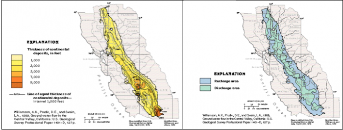
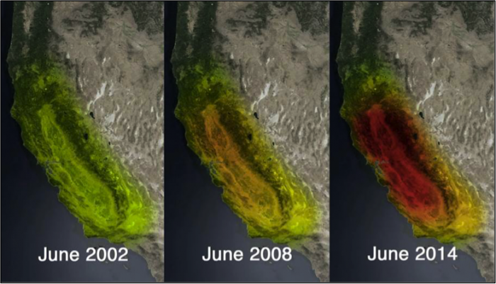
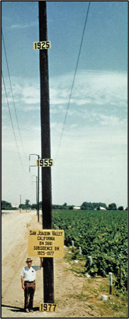
The thick sedimentary sequence has formed a vast expanse of flat topography on the natural floodplain of the San Joaquin River. This, in combination with a mild climate that allows a year-round growing season, has made the Central Valley one of the most productive and largest agricultural centers in the world. The Central Valley aquifer system is highly utilized, primarily to augment limited allocations of surface water for irrigation. Since the mid-1920s, groundwater withdrawals have generally outpaced natural recharge to the aquifer, leading to dropping water levels, irreversible aquifer compaction, and land subsidence (as will be discussed in more detail next week, in Module 6.2). Until recently, groundwater withdrawals were neither heavily monitored nor regulated. However, in the face of an ongoing multi-year drought, a new bill was signed into law in mid-September, 2014 that restricts pumping (See What to Know about California's New Groundwater Law [14]; see also New California Groundwater Pumping Rules Signed Into Law [15]). Shallow aquifer units in the valley are also plagued by a wide range of water quality concerns associated with irrigation and return flow of irrigation water to the aquifer via infiltration; these include leaching of selenium, boron, and other constituents from soils; salinization; and high concentrations of pesticides and fertilizers. We’ll discuss all of these issues in more detail in upcoming modules about water quality and the effects of climate change.
Darcy’s Experiments and Darcy’s Law
Darcy’s Experiments and Darcy’s Law
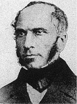
In 1855, Henri Darcy, a French hydraulic engineer (Figure 24), oversaw a series of experiments aimed to understand the rates of water flow through sand layers, and their relationship to pressure loss along the flow paths. Darcy’s experiments consisted of a vertical steel column, with a water inlet at one end and an outlet at the other. The water pressure was controlled at the inlet and outlet ends of the column using reservoirs with constant water levels (Figure 25) (denoted h1 and h2). The experiments included a series of tests with different packings of river sand, and a suite of tests using the same sand pack and column, but for which the inlet and outlet pressures were varied. For part of our in-class activity this week, we will perform our own set of “Darcy Tube” experiments, and also work with the original dataset generated by Darcy in his experiments.
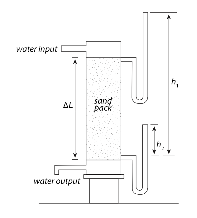
Darcy’s findings laid the foundation for the modern science of hydrogeology by quantifying the relationships between volumetric groundwater flow rate, driving forces, and aquifer properties. Specifically, Darcy’s experiments revealed proportionalities between the flux of water, Q, through the laboratory “aquifer” and different characteristics of the experimental system (refer to Figure 25 above):
(1) Q was directly proportional to the difference in water levels from inlet to outlet, h1 - h2 = Δh:
Q ∝ Δh
(2) Q was directly proportional to the cross sectional area of the tube:
Q∝ A
(3) Q was inversely proportional to the length of the column:
Q ∝ 1/ΔL
Combining these proportionalities leads to Darcy’s Law, the empirical law that describes groundwater flow:
Q = KA(Δh/ΔL)where K is a constant of proportionality that defines the water flux for a given hydraulic gradient (Δh/ΔL). The above equation can also be recast in terms of the water volume flux per unit area, Q/A (also called "Darcy flux" or "Darcy velocity" with units of length per time):
Q/A = K(Δh/ΔL)Note that in Darcy’s Law, the other terms all describe the driving forces or geometry of the experimental system; none of them would change if the sand pack in the tube were changed to gravel, silt, or another material. This is where the constant of proportionality, K, comes in: it describes the ability of the material in the column to transmit water (sound familiar?). Indeed, the constant of proportionality and hydraulic conductivity (also K) are one and the same! For example, consider the same experimental geometry, but with silt or clay in the tube rather than sand. The flow rate would be lower, and this would be described in Darcy’s Law by a smaller value of K.
6.2 Aquifer Processes and Dynamics
6.2 Aquifer Processes and Dynamics
In the first half of the module, we’ve explored the properties of aquifers. But, of course, that is only half of the story! In order for groundwater to flow, there must be a driving force. The same is true for surface water like streams or rivers: in that case, the driving force is gravity. In the case of groundwater, the driving force is a bit more complicated because it includes the combined effects of gravity and pressure.
As we will see, these driving forces are partly determined by the natural system but can be perturbed by pumping or injection in wells. When we pump water from wells, we alter the natural driving forces to move water toward the well. One important issue in aquifers is accounting for the flows in to and out of the aquifer in a groundwater budget. In extreme cases, the amount of water extracted at wells may exceed the amount introduced to the aquifer through recharge. As we’ll discuss, this tenuous condition is known as an overdraft.
Goals and Objectives
Goals and Objectives
Goals
- Describe the two-way relationship between water resources and human society
- Explain the distribution and dynamics of water at the surface and in the subsurface of the Earth
- Thoughtfully evaluate information and policy statements regarding the current and future predicted state of water resources
- Interpret graphical representations of scientific data
Learning Objectives
In completing this lesson, you will:
- Apply the concept of hydraulic head to draw flowlines on maps and cross-sections
- Interpret the current and historical balance between groundwater recharge and water extraction from well hydrographs
- Propose a course of action to address overdraft in an aquifer
Driving Forces for Groundwater Flow
Driving Forces for Groundwater Flow
The driving forces that control groundwater flow are a bit more complicated than those controlling flow in rivers and streams. As you learned in Module 3, surface water flows downhill due to gravity, and the flow direction is defined by the topography. Water flows downhill because gravity is a form of potential energy – and the water, or anything that falls or rolls downward – flows in response to differences in potential energy (from high to low).
In contrast to surface water, groundwater is separated from the atmosphere, and as a result, it can be under considerable pressure. Therefore, the potential energy that drives groundwater movement includes both pressure and gravity. In this section, you will learn about these driving forces, how we define them, and how they translate to the direction and rate of groundwater movement in the subsurface.
Potential Energy and Hydraulic Head
Potential Energy and Hydraulic Head
The flow of both surface water and groundwater is driven by differences in potential energy. In the case of surface water, flow occurs in response to differences in gravitational potential energy caused by elevation differences. In other words, water flows downhill, from high potential energy to low potential energy. In groundwater systems, things are a bit more interesting. Unlike surface water, which is in contact with the atmosphere and therefore rarely under pressure, water in groundwater systems is isolated from the land surface. This means that groundwater can also have potential energy associated with pressure. In extreme cases, water in confined aquifers may be under sufficient pressure to drive flow upward, against gravity. Artesian wells are one manifestation of this.
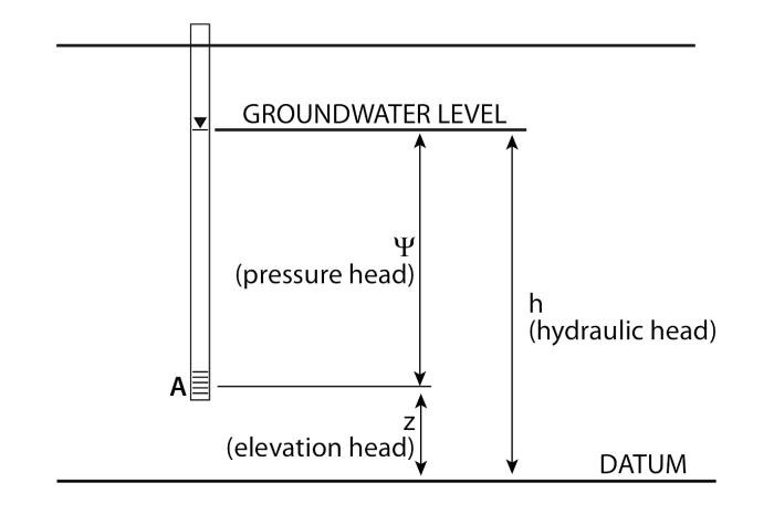
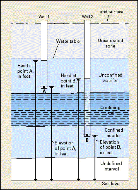
Fundamentally, groundwater and surface water are similar in that flow is in the “downhill” direction. But what does “downhill” mean in a groundwater system? To define the flow direction, we need to account for the two types of potential energy. Unfortunately, the potential energy of the water cannot be measured directly. However, we can measure a proxy for the potential energy by measuring the hydraulic head, or level to which water rises in a well (Figures 26 and 27). The hydraulic head combines two components: (1) potential energy contained by the water by virtue of its elevation above a reference datum, typically mean sea level; and (2) additional energy contributed by pressure. In a well, the value of hydraulic head represents the potential energy of the water at a particular point in three dimensions – at the depth where the well is open to the aquifer (Figures 26-27). This is analogous to a temperature reading taken at the tip of a thermometer, which provides a proxy for heat energy. Hydraulic head can be written as:
h = z + Ψ,
where z is the elevation energy, and Ψ is the pressure energy.
Click to expand to provide more information
Hydraulic Head and the Direction of Groundwater Flow
Hydraulic Head and the Direction of Groundwater Flow
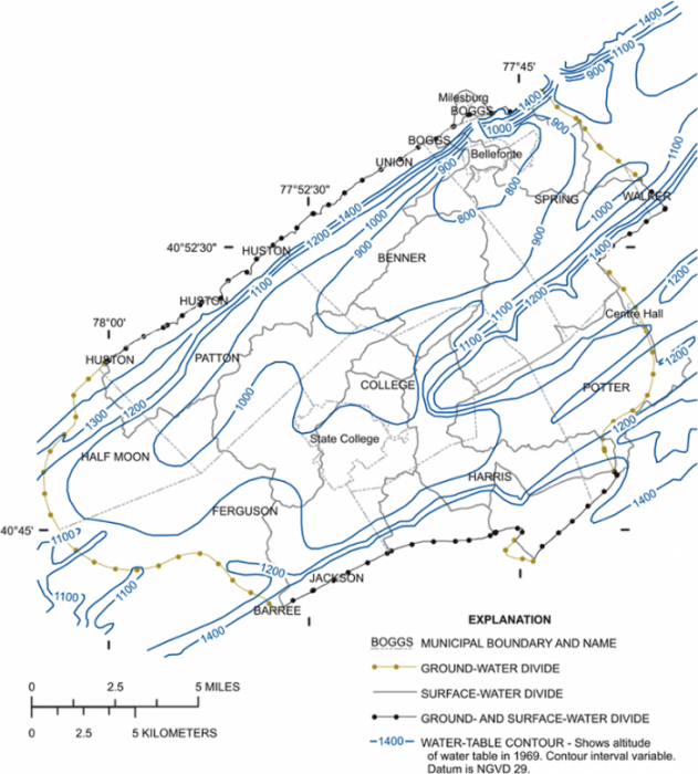
In order to define groundwater flow directions and rates through aquifers, individual measurements of hydraulic head are combined to generate contour maps of water level – or potential energy (Figure 29). These maps define the potentiometric surface, which is much like a topographic contour map but defines the distribution of potential energy in the groundwater system. Each contour, or equipotential, represents a line of equal hydraulic head.
To first approximation, groundwater flows down-gradient (from high to low hydraulic head). As is the case with surface water, or a ball rolling down a hill, the water flows in the direction of the steepest gradient, meaning that it flows perpendicular to equipotentials. There are exceptions to this – for example, if the hydraulic conductivity of the aquifer is much higher in one direction than another, or dominated by fractures with particular orientations, then these can redirect groundwater flow askew to the maximum gradient.
The potentiometric map also provides clues about the rate of groundwater flow. If you think back to Darcy material and our in-class activity from last week, you will recall that groundwater flow rate depends on the head gradient (i.e. the hydraulic gradient) and hydraulic conductivity. In a simple one-dimensional Darcy tube experiment, the head gradient is just the difference (h1-h2)/L. In two dimensions, the head gradient is defined by the slope of the potentiometric surface – just as the slope of the land surface is defined on a topographic map. The path that water takes in the aquifer, defined as a continuous line tracing the maximum gradient on a map of the potentiometric surface, is known as a flowline.
Well Hydrographs
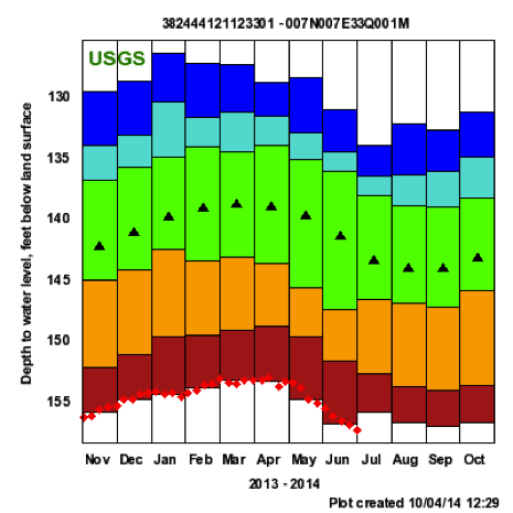
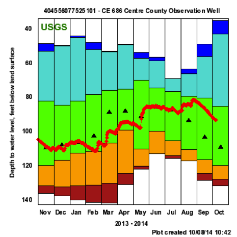
Well Hydrographs
Just as river hydrographs are used to record and visualize variations in flow with time (as discussed in Module 4), a well hydrograph is a time series of hydraulic head recorded in a well. This provides information about the fluctuation of hydraulic head (equivalent to the water table in an unconfined aquifer), which reflects the combined effects of temporal variations in climate, recharge, and pumping (Figures 30-31). The U.S. Geological Survey maintains a database of active monitoring wells [17] in major aquifer systems across the United States. Hydrographs provide information about seasonal patterns that may be associated with pronounced wet and dry seasons typical of some regions (for example, Central CA), as well as long-term trends driven by climate change, decadal-scale climate patterns like el nino, prolonged groundwater extraction, or human-induced modifications to natural recharge. We’ll cover examples of the latter two processes in the next section of the module (Module 6.2: Water budgets).
Effects of Pumping Wells
Effects of Pumping Wells
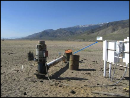
Groundwater is accessed by either pumping from wells drilled into the aquifer (Figure 33), or by developing natural springs where the potentiometric surface intersects the land surface (Big Spring in Bellefonte, PA is one example of a relatively large spring that is used for municipal supply). Although springs are relatively inexpensive to develop, they are not always present, nor are the flow rates always sufficient to support demand. As a result, most groundwater extraction occurs by pumping wells, or in many cases “fields” of wells concentrated in a small area.
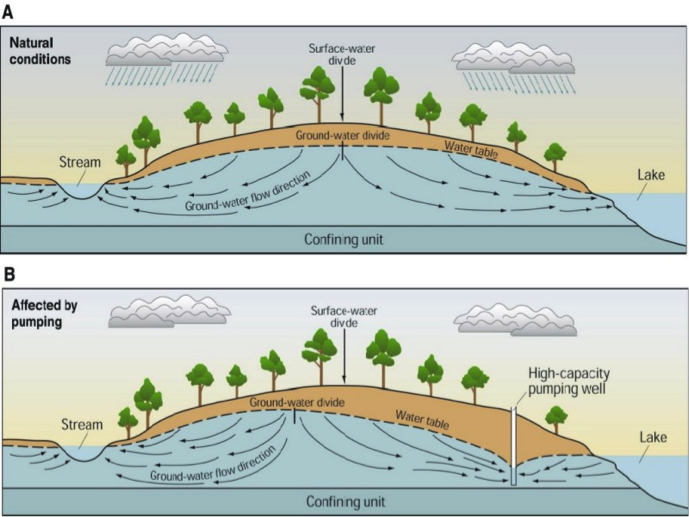
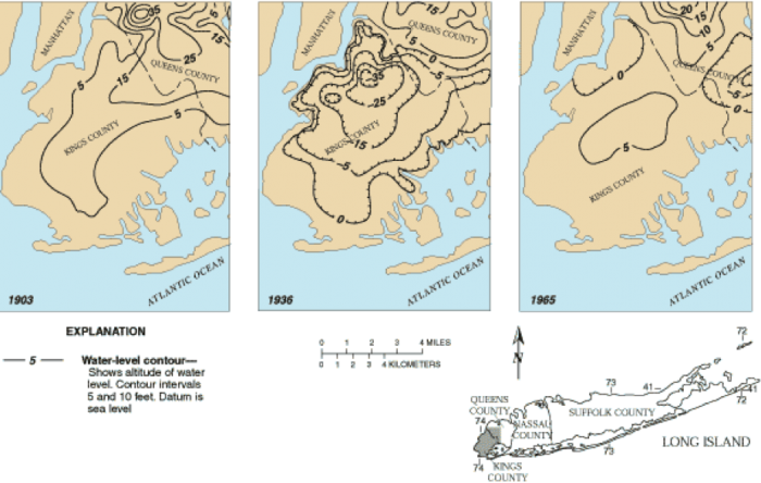
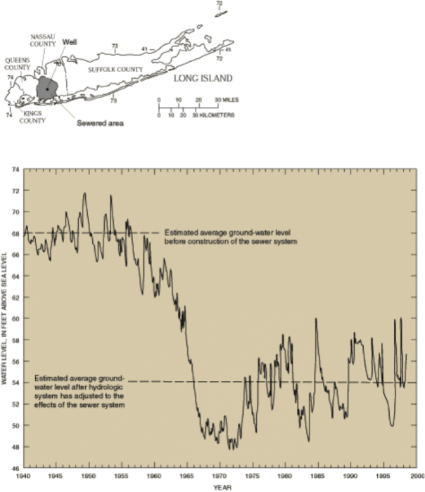
Cones of Depression: Pumping at a well, or at a wellfield, pulls water toward the well from all directions – in other words, it induces radial flow (around the radius of the well). In doing so, pumping causes a reduction in hydraulic head, known as drawdown. This drawdown generates a cone- or funnel-shaped depression called a cone of depression (Figure 35). The reduction in hydraulic head drives groundwater flow to the well (in the down-gradient direction), as shown in the example from Long Island in Figure 36.
Click for more information
Both the width and the depth of the cone of depression scale with the rate of pumping, the aquifer permeability, and storativity, and the duration of pumping. In general, larger cones of depression result from larger pumping rates, higher permeability or lower storativity, and longer elapsed time. If cones of depression from two separate pumping wells grow large enough to overlap, it is known as well interference. When well interference occurs, the respective drawdowns are added together. The result is that drawdown is accelerated when multiple cones of depression interact. This is generally not desirable, and is one important consideration in the design, permitting, and operation of wells.
Not only does the cone of depression draw water to the well, but if the pumping rate is large enough or pumping is sustained for a long time, it can reverse the natural hydraulic gradient hundreds of meters to several tens of km away from the well(s). In some cases, this may result in interception of groundwater that would normally feed a stream or river as baseflow, and even in the interception of streamflow itself by inducing infiltration in the stream bed or banks (Figure 35B). In other cases, large cones of depression (up to a few miles wide!) associated with industrial or municipal well fields may reverse regional topographically-driven hydraulic gradients and lead to problems like saltwater intrusion (Figure 35B).
Groundwater Budgets
Groundwater Budgets
Now that you are an expert on how groundwater flows, we will apply that knowledge to the important problem of groundwater budgets. As groundwater flows through and exits an aquifer, for example at springs or at extraction wells, those losses of water may be balanced by recharge that percolates from the land surface. As you’ll investigate in the following section, and through a case study of the famous Ogallala aquifer in the American Midwest, understanding the budget of inflows and outflows to an aquifer is critical to evaluating the sustainability of groundwater use.
Fluxes (Inflows and Outflows) in Groundwater Systems
Fluxes (Inflows and Outflows) in Groundwater Systems
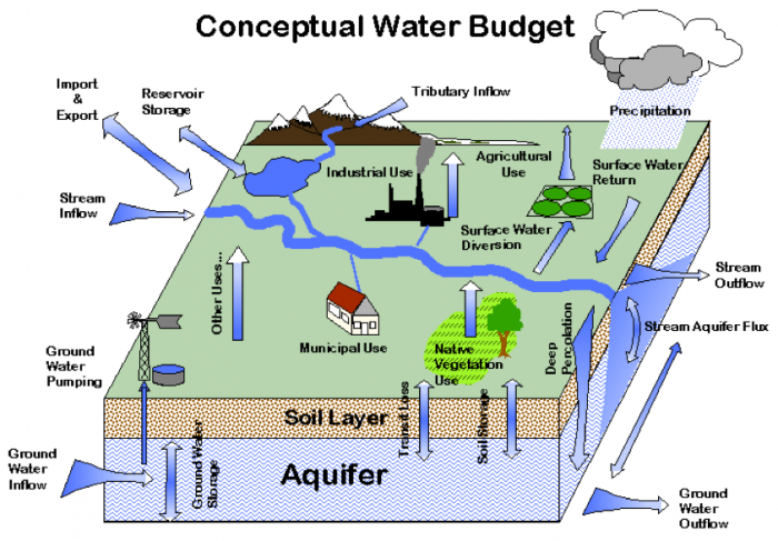
Fluxes (inflows and outflows) in Groundwater Systems: In order to define the water balance or water budget of an aquifer system, the individual processes that bring water into or out of the system must be quantified (Figure 37 on the next page).
Common inflows of water to a groundwater system include:
- Infiltration through the vadose zone that is not intercepted by evaporation, transpiration, or bound in the unsaturated zone, and thus becomes recharge. Infiltration may be distributed over large areas, or may be focused beneath surface water bodies or at geological features (e.g., sinkholes). Recharge may occur naturally or can be induced or enhanced by excavation and removal of low-permeability soils, and the construction of recharge pits, typically lined or filled with permeable sands (Figure 38 on the next page).
- Injection at wells, either for disposal of treated wastewater or as part of managed aquifer storage and recovery (ASR) programs. The latter is growing in popularity as one way to “bank” excess water in times of surplus, for example, wet seasons or wet years, and then tap the stored water when needed. Although energy-intensive because it requires pumping, ASR is not affected by evaporative losses whereas reservoirs are.
- Groundwater flow from areas outside of the region of interest – areas that are either up-gradient or above or below (i.e. flow across a confining layer).
Outflows from groundwater systems typically include:
- Evaporation or transpiration; this typically occurs in areas where the water table is shallow. Although direct evaporation of water from the water table is possible (in detail, this would occur by evaporation from the capillary fringe, and subsequent “wicking” of water upward from the water table), the upward flux (loss) of water from unconfined aquifers to the atmosphere is dominated by a family of plants known as phreatophytes, characterized by deep roots that extend to and below the water table.
- Water withdrawal by pumping from wells. As discussed in the previous section, pumping at wells induces radial flow toward the well. As the cone of depression grows, the well accesses water over a larger region of the aquifer. In some cases, as the cone of depression grows it may intercept water that would otherwise exit the aquifer via natural seeps or springs (e.g., Figure 37 on the next page), thus “redirecting” a flux that would have been an outflow somewhere else.
- Natural groundwater flow or discharge at springs or seeps, or to surface water bodies.
Surface Water-Groundwater Interaction
Surface Water-Groundwater Interaction
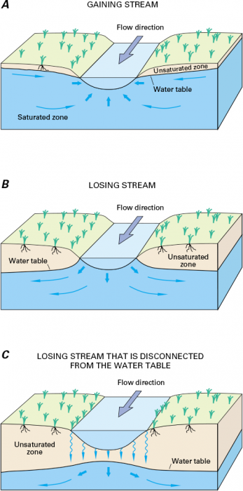
One specific class of inflow or outflow from groundwater systems results from surface water–groundwater interaction, water flows from aquifers into surface water bodies at seeps or springs, or infiltrates from rivers or lakes into aquifers (Figure 39; also note the dual-sided arrow between the aquifer and stream in Figure 37 indicating that the flux may be either to or from groundwater to surface water). If there is a net groundwater flux to surface water, the surface water body is said to be gaining (for example, a gaining stream is one that is fed by groundwater). As you may recall from Module 4, the component of streamflow derived from groundwater influx is termed baseflow. Alternatively, if the water table lies below the surface water body, the potential energy (hydraulic head) in the surface water body will be higher than in the groundwater system and water will percolate downward to the aquifer. In this configuration, the surface water body is said to be losing (i.e. a losing stream), because the stream or river discharge decreases downstream. While the land surface and stream channel generally remain at the same elevation, the water table commonly fluctuates over time (see Figures 32-33). As a result, it is common for streams to alternate between gaining to losing due to major recharge events, seasonality in precipitation and recharge, and variations in pumping rates.
Although water rights and policies are sometimes constructed with the implicit assumption that surface water and groundwater systems act independently, this is clearly not the case. A number of interesting situations arise from their interaction. As noted above in the Effects of Pumping Wells section, pumping at wells can reverse groundwater flow, and change a gaining stream to a losing one. In such a scenario, it isn’t always clear whether surface water rights are violated by groundwater pumping – even though groundwater extraction directly causes a reduction in surface water discharge, the water is withdrawn from the groundwater system, not the river. In large aquifer systems, the intercepted baseflow may impact users far downstream, across county and state borders. In other cases, also as noted earlier in this module, substantial or rapid influxes of surface water to groundwater systems, for example through fractures or sinkholes, can lead to groundwater contamination. If a direct connection between surface water and groundwater is demonstrated by the presence of microorganisms or increased water turbidity (cloudiness indicating suspended particles) in well water, additional treatment of groundwater is required before it is considered suitable for domestic or municipal use.
. At some depth below the land surface, the interstices between soil or sediment particles, or the fractures in the rock, will be water-filled or saturated. Shallower than that depth, these interstices, or pore spaces, will be filled with air, water vapor, and some liquid water bound to the surfaces of the rock (Figures 3-5). This zone is the unsaturated zone, also known as the “zone of soil moisture” or the vadose zone. The water table marks the top of the groundwater system, and is formally defined as the depth at which the pressure in the subsurface is equal to the atmospheric pressure. Immediately above the water table, there is a narrow zone of saturation termed the capillary fringe. In this zone, water is wicked upward in pore spaces due to capillary forces. This is analogous to capillary tube experiments you may have seen or performed in physics or chemistry classes in high school; it occurs due to interaction between the polar water molecule and the surfaces of the solids, and is directly related to the fact that water has a surface tension (as you may remember from Module 1!). In the capillary fringe, pores are saturated, but pressures are sub-atmospheric, meaning that the water is under suction as it is pulled or wicked upward. The nomenclature “fringe” reflects the fact that slight variations in grain size lead to variations in the height that water is drawn (again, think to the capillary tube experiment, and effects of different tube sizes) (Figure 5).</p> <p>Any precipitation or surface water that infiltrates to the water table must percolate through the vadose zone in order to recharge the aquifer. As we will see later in this module infiltration and recharge typically constitute only a small fraction – rarely more than 10% - of precipitation, because most water that falls in events is returned to the atmosphere by transpiration or evaporation, becomes runoff (i.e., if the capacity for infiltration is exceeded by the rate of precipitation), or is bound by soils in the vadose zone.</p> <div class="img-center"><img alt="Diagram of vertical section from land surface through vadose zone, capillary fringe, and into unconfined aquifer." src="/earth111/sites/www.e-education.psu.edu.earth111/files/Module6/Earth111Mod6AFig2left.png" /> <div class="img-caption">Figure 3. Schematic diagram showing vertical section from the land surface through the vadose zone, capillary fringe, and into an unconfined aquifer.</div> <div class="img-credit">Source: From W.M. Alley et al., 1999, <a href="http://pubs.usgs.gov/circ/circ1186/index.html">USGS Circular 1186: Sustainability of Groundwater Resources</a></div> </div> <div class="img-center"><img alt="Illustration of capillary action; water drawn to different heights in tubes of different internal diameters." src="/earth111/sites/www.e-education.psu.edu.earth111/files/Module6/Earth111Mod6AFig2right.png" /> <div class="img-caption">Figure 4. Illustration of capillary action; water is drawn to different heights in tubes of different internal diameters.</div> <div class="img-credit">Source: From <a href="http://water.usgs.gov/edu/capillaryaction.html">USGS Water Science School</a>. Photo Credit: C. Robinson, West Texas A&M Univ.</div> </div> <div class="img-center"><img alt="Cross sectional diagram of water table aquifier." src="/earth111/sites/www.e-education.psu.edu.earth111/files/Module6/Earth111Mod6AFig3_0.png" /> <div class="img-caption">Figure 5. Cross sectional diagram of a water Illustration of capillary action; water is drawn to different heights in tubes of different internal diameters, showing the vadose zone (unsaturated zone), water table, and saturated aquifer. Insets below show water occurrence in crevices or fractures in rock (left) or between sediment or soil grains (right).</div> <div class="img-credit">Source: U.S. Geological Survey, <a href="http://water.usgs.gov/edu/earthgwaquifer.html">Water Science for Schools: Aquifers</a>.</div> </div>)
Water Budgets
Water Budgets
The balance of water inflows and outflows, or water budget, for a groundwater system, is described by a simple equation:
where I is the total of the inflows to the system, O the total outflows and ΔS is the change in storage. The water balance equation is no different than a bank statement: the difference between deposits (inflows) and withdrawals (outflows) is equal to the change in the account balance (storage). In the case of groundwater systems, changes in storage are manifested as changes in the potentiometric surface, either due to drop in the water table (in unconfined aquifers) or reduction in elastic storage as aquifer is depressurized (in confined aquifers).
In a steady state, or equilibrium condition, inflows and outflows are perfectly balanced (i.e. I = O in the budget equation above), and ΔS is zero. In other words, the potentiometric surface is steady. Often, groundwater systems are considered to be at steady state if inflows and outflows balance over a yearly or decadal timescale. This is because, in many aquifers, both recharge and extraction may be strongly seasonal. For example, recharge in many aquifers in the western US is mostly restricted to the winter months when precipitation is highest, and withdrawal rates are highest in the summer and early fall dry season. As a result, the potentiometric surface may fluctuate over the course of the year but is more-or-less constant over the long-term.
A variety of processes can lead to non-steady state conditions. Most notably in aquifers that are used heavily for irrigation, industry, or municipal supply, pumping may significantly exceed recharge, leading to net decreases in storage. In other cases, reduced recharge – for example due to urbanization and construction of impervious surfaces that do not allow infiltration, removal of leach fields upon installation of sewers (Figure 30), or long-term climate trends that drive changes in the amount or timing of precipitation – also results in negative changes in storage. Reductions in groundwater extraction, or periods of increased precipitation, will have the opposite effect and lead to increases in storage.
Overdraft
Overdraft
Groundwater overdraft is a specific condition in which extraction greatly exceeds the influxes of water (mainly recharge). This produces an unsustainable condition characterized by sustained declining water levels. Much like overdraft of a bank account, groundwater overdraft is not a desirable state of affairs. Not only is it unsustainable in terms of management of the groundwater resource, but it also leads to long-lasting damages (a lot like what happens to your credit rating if your bank account is overdrafted!).
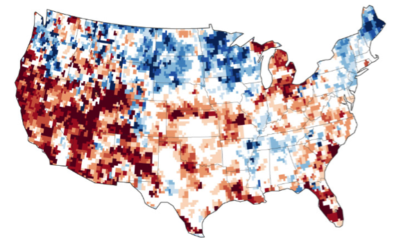
Depressurization of the aquifer, if large enough, may cause irreversible collapse and compaction. This reduces both storage (porosity) .and hydraulic conductivity. It can also lead to land subsidence, especially in cases where the magnitude of overdraft is large and the aquifer units are thick and highly compressible, as is common for unconsolidated or uncemented sedimentary aquifers. One well-known example of groundwater overdraft is the Central Valley of California (Figure 41). Another is the Ogallala aquifer, a major groundwater system spanning across eight states in the American Midwest (Figure 43; see The High Plains Aquifer section). Substantial overdraft and subsidence also occur in widespread areas of the southeastern U.S., the Gulf Coast, and parts of Arizona and Las Vegas (Figure 44).
The High Plains Aquifer
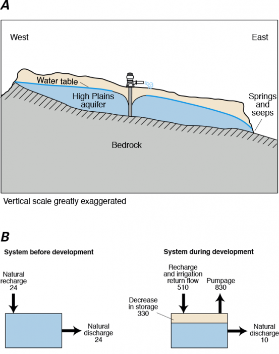
The High Plains Aquifer
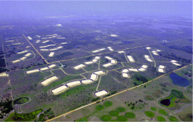
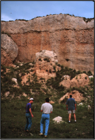
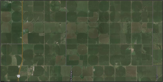
The High Plains Aquifer system consists of Tertiary sedimentary rock, dominantly sandstone and gravel (Figure 45), eroded from the ancient Rocky Mountains and deposited in the Tertiary period (from about 31 to 5 million years ago). The Ogallala Formation is the primary aquifer unit in the system. The aquifer underlies almost 175,000 mi2 and spans eight states, with most of its area in Nebraska, Texas, and Kansas. This region is among the largest and most productive croplands in the U.S. and is the source of almost 20% of our corn, wheat, and cotton production, as well as a significant portion of our soybeans, sorghum, and alfalfa. It is also host to almost 20% of the cattle raised in the US. Because the climate is semi-arid, with mean annual precipitation ranging from 12 inches in the West to 33 inches in the East, growing economically viable crops requires substantial irrigation. If you have ever flown over the Midwest on a clear day you may have seen circular “patches” of irrigated land - the hallmark of center-pivot irrigation systems (Figure 46).
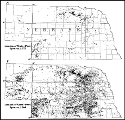
Although farming has been a major part of the economy in the region since the late 1800s, in the 1960’s new technology in electrical pumps allowed access to deeper groundwater and ushered in an era of rapidly expanding irrigated acreage (Figure 47). Accompanying this expansion, aquifer-wide groundwater withdrawals increased from a few million acre-feet (M-AF) per year to almost 20 M-AF. Water level declines began in the 1950s, with the onset of intensive groundwater extraction for irrigation-based agriculture. The total overdraft of the aquifer is almost 250 million acre-feet, from pre-development (ca. 1950) to 2011 – this is almost 17 times the annual flow of the Colorado River.
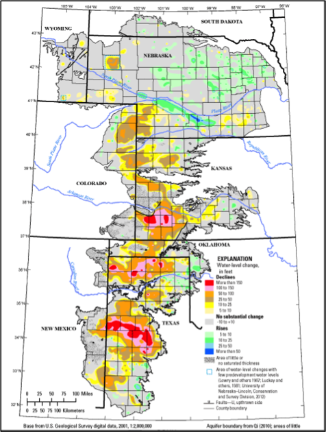
As a consequence of sustained overdraft for several decades (see Figure 42 above), water levels in the aquifer have dropped substantially, by more than 100 feet in many areas (Figure 48). Over half of this decline has occurred since 2000. Water level declines are not evenly distributed, however. The highest rates of decline are focused in the southern reaches of the aquifer system, where recharge rates are low and irrigation demand is highest. In the northern portions of the aquifer system, water level declines are considerably smaller – and in some cases, the water table has actually risen – primarily due to locally higher recharge focused along the Platte River (Figure 48).