Making Sense of Hydrologic Variability
Making Sense of Hydrologic Variability
Video: Advanced Hydrologic Prediction Service (1:37)
This short video introduces the NWS Advanced Hydrologic Prediction Service that provides alerts for droughts and floods in the United States.
Montra Lockwood - Forecaster, National Weather Service, Lake Charles, LA: Floods are one of nature's deadliest natural disasters. Timely and accurate forecasting of floods is vital to the protection of life and property. The Advanced Hydrologic Prediction Service, also known as AHPS, was created for this purpose.
AHPS is a national weather service program designed to provide improved river and flood forecasting. This service provides a suite of text and graphical products that are available online to assist the public, community officials, and emergency managers, in making better life and cost-saving decisions about evacuations and protection of property before flooding occurs. AHPS provides detailed and accurate answers to such questions as, How high will the river rise? When will the river crest? Where will it flood? How long will the flood last? How certain is the forecast? and What are the impacts of the flood? Additional enhancements to the AHPS pages include multi-sensor precipitation information and flood inundation maps for specific locations. To view AHPS information, please visit the AHPS website at water.weather.gov/AHPS. And for more information on flooding and what you can do to protect yourself and your property, visit the National Weather Service's Flood Safety page at nws.noaa.gov/floodsafety.
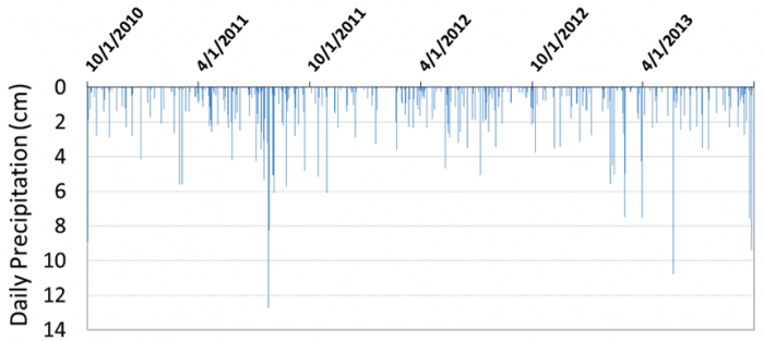
Precipitation and streamflow are both incredibly variable aspects of the environment, often changing dramatically over short time scales and small spatial scales. If you look up the precipitation record for a location of interest (data freely available from the National Weather Service, Natural Resource Conservation Service, and many other outlets), you would see that events seem to happen ‘randomly’, often without an obvious pattern in the frequency, magnitude or duration. Take, for example, the precipitation record for Kingston, New York from October 1, 2010, through September 30, 2013 (Figure 1). There is an immense amount of variability from day to day. So what can we really say about precipitation from these data? July and August of 2011 appear to be a very wet time period, with many events clustered and one event reaching over 12 cm (nearly 5 inches)! Do you think that caused a flood? Precipitation was very sparse from mid-December 2011 to mid-February 2012. Do you think that was a drought?
It is essentially impossible to answer the questions posed above about July 2011 being a flood or winter 2011-2012 being a drought from the precipitation data alone because precipitation is not the only factor that causes floods and droughts. Processes of water use and transport occurring in a landscape also matter. For example, an increased impervious surface associated with urbanization is known to dramatically increase runoff, resulting in much higher peak discharge (bigger floods) for any given amount of rainfall. In contrast, a large rain event occurring on dry soil will have a relatively small effect on streamflow compared with the same rainfall event occurring on very wet or saturated soils, because more of the rain would be absorbed by the dry soil. Landscape processes also influence droughts. While a prolonged lack of precipitation can initiate a drought, the severity of the drought is strongly influenced by the water demand, by vegetation and/or humans, throughout the landscape. Landscape processes can amplify or dampen precipitation variability. This greatly complicates the job of forecasting floods and droughts. Hydrologists must account for numerous factors that vary in time and/or space.
Though it is difficult, hydrologists can make remarkably accurate and timely predictions of floods and droughts. For example, the National Weather Service (NWS) uses large amounts of real-time data from precipitation gauges, radar systems, river discharge gages, and satellite imagery. The NWS maintains a network of 13 river forecast centers and 50 hydrologic service areas that provide real-time flood warnings throughout the US, which can greatly reduce loss of life and property damages.
| Date | Daily Precipitation (cm) |
|---|---|
| October 1, 2010 | 3 |
| April 1, 2011 | 2.25 |
| October 1, 2011 | 5 |
| April 1, 2012 | 1.5 |
| October 1, 2012 | 3.75 |
| April 1, 2013 | 7.5 |
Forecasting and Predictions
Forecasting and Predictions
Meteorologists have made excellent progress in the past few decades to improve our abilities to forecast when rain events might occur over the next week or so, which facilitates the short-term forecasting of floods and droughts discussed in the paragraph above. However, complex atmospheric dynamics prevent forecasts beyond more than a few weeks in advance. Nevertheless, we must have some basis for making decisions about development, infrastructure and agriculture (e.g., How big should we build a culvert under a road? What size retention basin is needed next to a new housing development? Which agricultural fields will require artificial drainage and which will require irrigation?).
For these longer-term predictions we can use statistics to determine how likely it is that a given location will experience, for example, more than 10 cm of rain in a day, or less than 5 cm of rain during a given month. Many million- and billion-dollar decisions about development and infrastructure are based on such predictions.
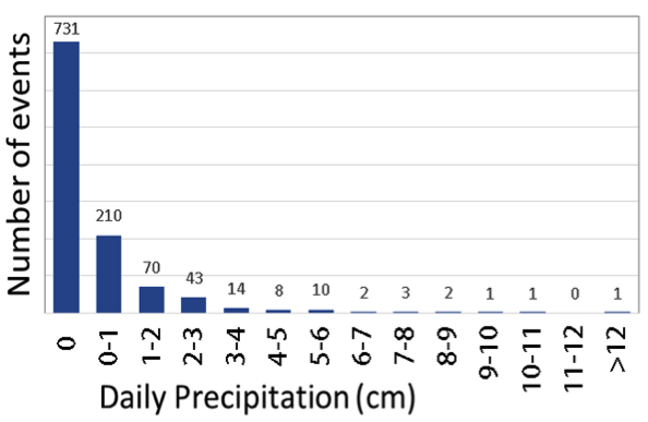
To make these predictions, hydrologists synthesize historical data and use a statistics-based approach to determine the likelihood that a given event might occur. While Figure 1 highlights the ‘messiness’ of precipitation events over time, reorganization of the data provides useful information. Figure 2 shows a histogram of the precipitation data presented in Figure 1. A histogram is a plot showing the number of events that fall within chosen data groups or “bins” (shown on the x axis). From these data you can quickly determine that Kingston, NY experiences no rain about 2 out of every 3 days (731 out of the total 1096 days in this record). Only 10 days in the record had rainfall that exceeded 6 cm, so from these data alone you would expect such large rainfall events to happen 10 days out of 1096, or about 1% of the time. On 210 days during this time period the amount of rainfall was between the minimum measurable (typically 0.025 cm or 0.01 inch) and 1 cm (0.4 inches).
Hydrologists tend to use the term ‘forecast’ when referring to a future projection for which we have a lot of information (and therefore relatively high certainty of when an event might occur and what magnitude it might be). In contrast, hydrologists use the term ‘prediction’ for future projections for which less information is available, and therefore uncertainty is greater.
| Daily Precipitation (cm) | Number of events |
|---|---|
| 0 | 731 |
| 0-1 | 210 |
| 1-2 | 70 |
| 2-3 | 43 |
| 3-4 | 14 |
| 4-5 | 8 |
| 5-6 | 10 |
| 6-7 | 2 |
| 7-8 | 3 |
| 8-9 | 2 |
| 9-10 | 1 |
| 10-11 | 1 |
| 11-12 | 0 |
| >12 | 1 |
Learning Checkpoint
The National Weather Service maintains a Precipitation Frequency Data Server (PFDS) website [1] that allows you to look up the frequency of precipitation events of different duration and magnitude for most locations in the US. The PFDS website will open in a new window. Peruse the website and answer the following questions:
Zoom in on Logan, Utah and place the red crosshair directly over Logan. Below the map a table will appear showing the amount of precipitation associated with a range of time periods (durations shown in left column, ranging from 5 minutes to 60 days) and the average frequency with which such an event might happen (the recurrence interval, listed in years).
1. What is the amount of precipitation that you would expect to get in Logan, Utah on an annual basis, within a 24 hour time period?
(a) 0.1 inches
(b) 0.7 inches
(c) 1.2 inches
(d) 2.4 inches
ANSWER: (c) 1.2 inches
2. What is the amount of precipitation that you would expect to get in Logan, Utah on an annual basis, within a 60 minute time period with a frequency of once every 10 years?
(a) 0.1 inches
(b) 0.7 inches
(c) 1.2 inches
(d) 2.4 inches
ANSWER: (b) 0.7 inches
Zoom in on Chickamauga, Georgia and answer the following questions.
(a) 0.1 inches
(b) 1.3 inches
(c) 2.1 inches
(d) 3.3 inches
ANSWER: (d) 3.3 inches
4. What is the amount of precipitation that you would expect to get in Chickamauga on an annual basis, within a 60 minute time period with a frequency of once every 10 years?
(a) 0.1 inches
(b) 1.3 inches
(c) 2.1 inches
(d) 3.3 inches
ANSWER: (c) 2.1 inches
Predicting Frequency and Magnitude
Predicting Frequency and Magnitude
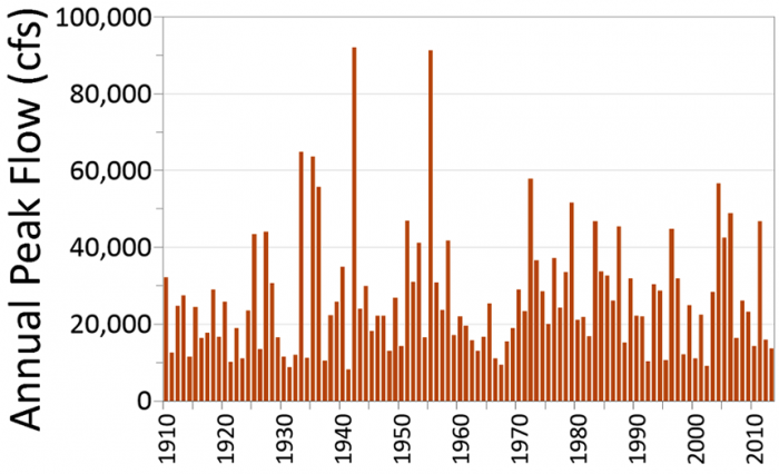
We can do similar calculations to estimate the frequency and magnitude of floods. For example, Figure 3 shows the annual maximum series of flows for the Lehigh River at Bethlehem, PA from 1910 to 2013. The annual maximum series is simply the highest flow value recorded for each year (typically for the water year, October 1 – September 30 as discussed in module 3). The largest flow on record (92,000 cfs) occurred in 1942 (on May 23, to be exact). Note that these are daily flow values which average flow over the course of the entire day, so the actual peak that occurred on May 23 was probably slightly higher. Interestingly, the year that had the smallest peak discharge on record was April 6, 1941 (only 8210 cfs, less than 10% of the whopper flood that came through the following year). But note that we are still talking about the highest flow for that particular year, which is still considerably higher than the average annual flow which is about 1,300 cfs. How can we use this information to predict what might happen in the future to support decisions about development, flood risk, or factors that may influence biota in the river or floodplain (e.g., factors limiting the return of certain fish)?
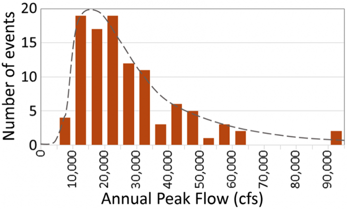
Similar to the precipitation example above, it helps to reorganize the data. The histogram shown in Figure 4 illustrates the frequency of events in 19 different “bins”. For example, the Lehigh River at Bethlehem, PA has never experienced an annual peak flow less than 5,000 cfs, so there is no orange bar in that bin. But it has experienced 4 peak flows that fall between 5,000 and 10,000 cfs. It has experienced a total of 55 peak flows that fall within the range of 10,000 to 25,000 cfs. These are the most common peak flows for the Lehigh River. And you can see the two outliers at the high end (92,000 cfs in 1942 and 91,300 cfs in 1955).
Typically, hydrologists will approximate the distribution of events that you see in Figure 4 as a probability density function, represented by the smooth, dashed-grey curve superimposed on the plot. This allows them to integrate under the curve above a value of interest to determine the probability that a flood of that magnitude (or larger) will occur. For example, integrating to find the area under the grey dashed curve above 60,000 cfs in Figure 4 would tell you the probability in any given year (in the future) that a flood of that magnitude (or larger) will occur. From that information, you can build your bridge to the appropriate size, or set your flood insurance rates accordingly, etc. Calculating probabilities associated with floods of a given magnitude is discussed in greater detail in the exercise associated with this module.
The same general principles apply to studying droughts. However, as we discuss below, droughts are more difficult to define and quantify because they build up over time and vary immensely over any given area. Nevertheless, similar plots of drought frequency, severity and duration can be developed for droughts, similar to Figure 4, to make sense of all the messy variability we observe in water deficiencies. With this brief introduction hopefully you can appreciate the great challenges in predicting the occurrence and severity of floods and droughts, and you can begin to see the implications for socio-economic systems and ecosystems.