Water Moves Through the Landscape
Water Moves Through the Landscape
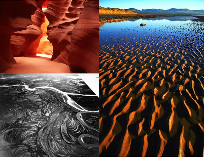
The most obvious way water moves through a landscape is via stream and river channels. There is no formal definition to distinguish between brooks, creeks, streams, and rivers, but generally speaking, the former terms refer to smaller waterways and the latter refer to larger waterways. The terms stream and river are often used interchangeably. There are over 3.5 million miles (5.6 million kilometers) of streams and rivers in the US. If all the streams and rivers throughout the US were lined up one after the next, they would extend the distance from Earth to the moon and back...seven times! That is an incredible length of streams to be monitored, protected, regulated, and (occasionally) repaired by federal, state and local agencies, as well as industry and non-profit organizations and individuals. In addition, streams sculpt much of the surface of the Earth, forming a multitude of beautiful patterns and awe-inspiring features, as shown in Figure 1.
Channel Networks and Watersheds
Channel Networks and Watersheds
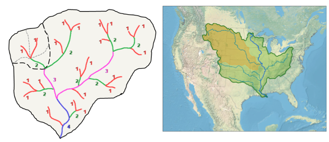
Streams naturally assemble themselves into surprisingly well-organized (quasi-fractal) networks. Figure 2 shows a typical channel network where many small streams converge to make progressively larger streams. The smallest streams in the network, which have no other streams flowing into them, are referred to as first order streams. When two first order streams meet, a second order stream is formed. When two second order streams meet, they form a third order stream, and so on. According to this conventional stream ordering system, first developed by Horton (1945) and refined by Strahler (1957), when a smaller order stream (e.g., first order) meets a larger order stream (e.g., second order), the resulting stream retains the order of the larger stream (in this case, second order).
Each stream has a watershed, also known as a ‘river basin’ or ‘catchment’ because it is the land that ‘catches’ precipitation and funnels it towards the stream. The watersheds of two first order streams are outlined with grey dashed lines in Figure 2. The watershed of a second order stream is outlined in black dashed lines and encompasses the two first order watersheds. The solid black outline in Figure 2 shows the watershed boundary for the fourth order watershed, which encompasses all other watersheds nested within it. The right side of Figure 2 shows the Mississippi River watershed highlighted in green, with the Missouri River watershed nested within it, highlighted in orange. By the time the Mississippi River reaches New Orleans, it is a tenth order stream (though only a few of its largest tributaries are shown in Figure 2), and drains more than one-third of the contiguous US.
The concept of connectivity between rivers and their watersheds will come up again towards the end of this module in the context of restoration. If a particular stretch of stream is impaired for one function or another (e.g., fish habitat has been degraded), in some cases it makes sense to ‘fix’ that specific stretch of river, while in other cases the impairment is simply a symptom of problems higher up in the watershed, so the ‘fix’ may need to be applied at that location in the watershed before human intervention or natural processes can begin to repair the impaired stream. Such is the way that watersheds and streams are connected.
Watersheds are Complex Systems
Watersheds are Complex Systems
When you look around, you see that the world is full of systems…assemblages or combinations of things that form a functional unit. Some systems are human-made, others are made by nature. Some systems are simple, meaning the way they work is straightforward and the outputs from the system are easily predictable. Other systems are complex, meaning they often have many parts that interact, often in non-linear ways, making the outputs from those systems more difficult to predict.
For example, a coffee maker is a pretty simple system. You put in 8 cups of water and two cups of coffee grounds and (assuming you put them in the right places), you turn the machine on and get ~8 cups of coffee. If you change the amounts of either of the inputs, it is pretty easy to predict the impacts on the coffee you brew.
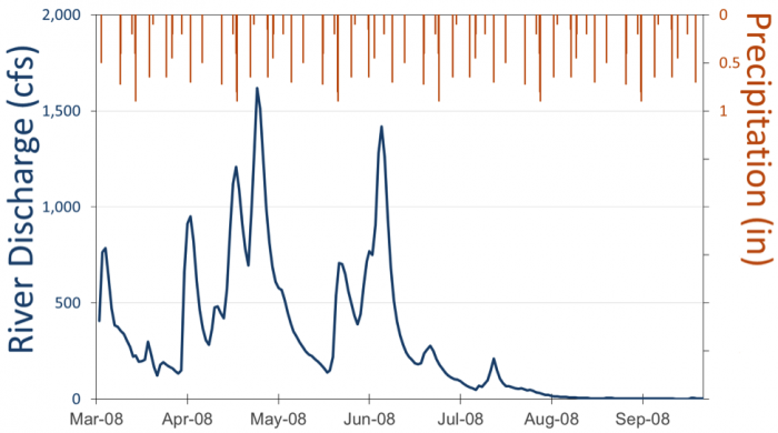
Watersheds are not such a simple system. They are incredibly complex. One example can be seen in how the relationship between rainfall and runoff changes throughout the year. In a simple system, you would expect a constant relationship between incoming rainfall and outgoing flow. For example, a 1-inch rain event should translate to a stormflow hydrograph that might last 2 days and peak at 1000 cfs. But this isn’t what we see. Figure 3 shows streamflow (blue line, values on the left axis) and precipitation (orange bars, values on the right axis) from March through September 2008 for the Maple River near Rapidan, Minnesota. Precipitation is relatively evenly distributed throughout the year. As you can see, in April and May, rainfall events that are 0.5 to 1 inch result in relatively high flows (1000 to 1500 cfs). However, in July, August, and September, similar rainfall events hardly elicit any flow response whatsoever! Why do we see such non-linear behavior?
Activate Your Learning
The Maple River example above is a relatively extreme example of changes in rainfall-runoff relationships because soils are relatively wet (and therefore can’t absorb much of the incoming rainfall) in the spring and there is very little vegetation to intercept or evapotranspire water (the watershed is covered in row crops that don’t grow much before mid-June). In contrast, the row crops are in full effect by mid-summer and early fall and therefore they dry out the soil, intercept some incoming rainfall and evapotranspire most of the rest of the incoming rainfall…so it never gets to the channel! But similar phenomena can be seen in other watersheds. Find precipitation and streamflow data for a watershed of interest to you (from the USGS website, NRCS SNOTEL website, or NWS website). Plot them as shown in Figure 3. How well does flow correlate with precipitation? Are there seasonal differences? Differences from year to year?
ANSWER - NEED ANSWER OR TALKING POINTS.
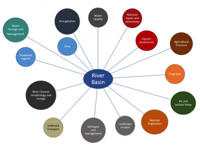
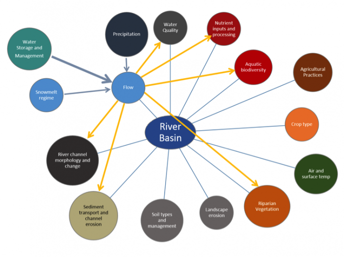
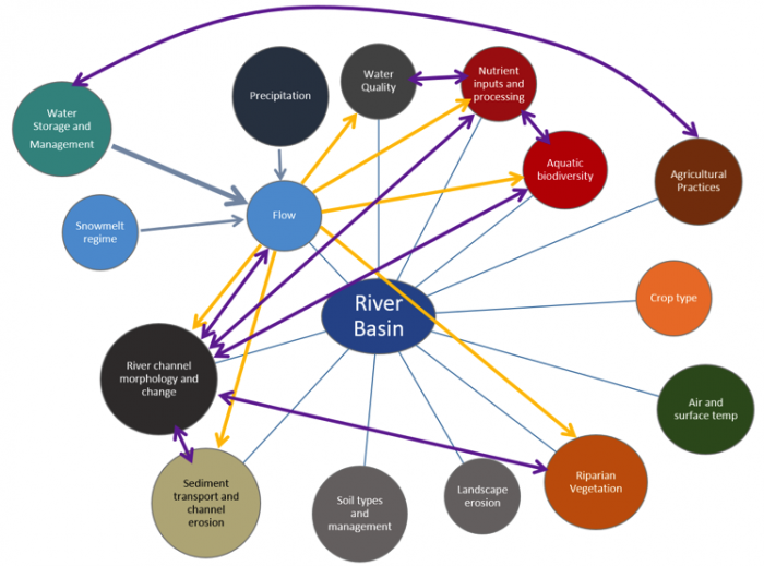
Watersheds comprise many interacting parts. Figure 4 (top panel) is one way to represent various ‘parts’ that might be considered to comprise the watershed. While this is clearly a very simple view of this complex system, it is useful to take a “crude look at the whole”, a term coined by Nobel Prize-winning Physicist Murray Gell-Mann, as a starting point. When one component of the system is systematically changed, it may have direct as well as indirect impacts that propagate through the system. For example, changes in precipitation, snowmelt regime, or water storage may change streamflow. This altered streamflow has direct effects on river channel morphology, sediment transport, riparian vegetation, water quality, nutrient processing, and biodiversity, as indicated by the yellow arrows in the middle panel of Figure 4. But there are other interactions within the system, feedbacks that are indicated by purple arrows in the bottom panel of Figure 4. So to predict impacts of the changes in flow on aquatic biodiversity you would have to take into account not only the direct effects (yellow arrow between flow and aquatic biodiversity, but also the indirect effects associated with changes in channel morphology. This concept is also relevant in the context of watershed ‘restoration’. If a particular stretch of stream is impaired for one function or another (e.g., fish habitat has been degraded), in some cases it makes sense to ‘fix’ that specific stretch of river, while in other cases the impairment is simply a symptom of problems higher up in the watershed, so the ‘fix’ may need to be applied at that distant location in the watershed before human intervention or natural processes can begin to repair the impaired stretch of stream.
These notions of complex feedbacks and cascading effects greatly complicate the process of predicting what impacts human activities or natural disturbances within a watershed might have downstream. We’ll come back to this theme of system dynamics and complexity throughout the course.
Streams
Streams
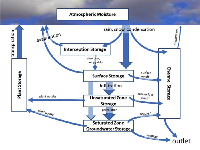
Streams are the most obvious way that water is moved through a watershed because we see them all over. But there are many other means by which water moves, as discussed in module 2. Figure 5 illustrates the various stocks (places were water is stored, even if only temporarily) and fluxes (mechanisms by which water moves) of water that may exist within any given watershed. For example, one raindrop might fall onto vegetation (called interception) and subsequently be evaporated back up into the atmosphere. Another raindrop might fall onto the soil surface and then runoff the surface into the stream channel or it might infiltrate down into the soil. Once in the soil, the water might further percolate down into the groundwater, where the soil or rock is saturated with water. Alternatively, once in the soil, the water might travel downhill within the soil and runoff into the stream or it might be taken up by vegetation and transpired back into the atmosphere. Estimating and predicting which, and to what extent, water travels through these pathways is an active field of hydrologic research and is also vitally important for environmental management and policymaking, as certain pathways may be more or less prone to filtering or polluting water along its journey to the place where you might want to use it for drinking, irrigating, fishing, swimming or the myriad other purposes for which we need water.