River Flow Changes Over Time
River Flow Changes Over Time
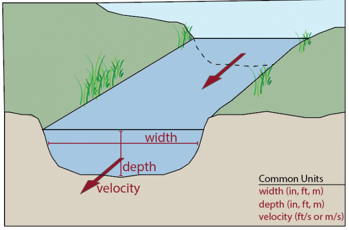
The amount of water moving down a river at a given time and place is referred to as its discharge, or flow, and is measured as a volume of water per unit time, typically cubic feet per second or cubic meters per second. The discharge at any given point in a river can be calculated as the product of the width (in ft or m) times the average depth (in ft or m) times average velocity (in ft/s or m/s).
The vast majority of rivers are known to exhibit considerable variability in flow over time because inputs from the watershed, in the form of rain events, snowmelt, groundwater seepage, etc., vary over time. Some rivers respond quickly to rainfall runoff or snowmelt, while others respond more slowly depending on the size of the watershed, steepness of the hillslopes, the ability of the soils to (at least temporarily) absorb and retain water, and the amount of storage in lakes and wetlands.
Video: How to Measure a River (8:35)
Good morning. I'm Barry, I'm Ben. We're the Geography Men.
Ben: Now today I'm going to be showing you how to measure the discharge of a river. Now for this what you're going to need is a tape measure, a meter stick, a flowmeter, a couple of stakes to help you out, and a recording sheet to record your data.
So the first thing you're going to want to measure is the width of the river. Now as I said before, for this you're going to need a tape measure, preferably let's say a 30-meter tape measure. Now from the left-hand bank, you want to have your 0-end of your tape measure. The easiest way to do this is to tie it to something or to use a stake in the ground. Now here I'm going to tie it to this root just to help me out. Now you want to stretch the tape measure across the river, making sure that it is tight across the surface of the water. You do not want to allow it to go slack, otherwise, that tape is going to get carried off by the river and you are going to get a false measurement of the width of your river.
Now that you have your tape set across your river, you want to record where the river begins, where the water meets the bank. Record on the other edge, on the other bank, where the water meets the bank, and then work out that distance from one bank to the other.
With this river here, our left-hand bank starts at 1 meter 60 and our right-hand bank ends at 5 meter 60, giving us a width of our river of 4 meters. Now the next thing we need to do with that width is we need to divide it by 11, in order to work out the intervals at which we need to work out the depths of our river. The reason we divide it by 11 is because we're going to take a measurement at each of the banks. This will give us 10 intervals across our river to take our depth.
Now for our depth, we're going to want to use a meter stick. Now with the meter stick, there's some very simple things that you need to remember. Number one, make sure the zero end of the stick is at the bottom of the river. You don't want to have it upside down and be getting readings of 80 or 90 centimeters. You want to turn the meter stick parallel to the flow of the water, so as that meter stick does not block that flow of the water giving you two false values on either side. Starting at the bank, place that meter stick into the water until it reaches the bed of the river. Now you want to take a reading and you want to convert that reading straight into meters, as you want the same units for each of your measurements. So here we have 25 centimeters, so we have naught .25 meters. Find your next interval on the tape and do exactly the same again. We have naught .21. Naught .24. And you would then follow that across the river until you reach the right-hand bank.
Now the final measurement you want to take at your site, to work out the discharge of the river, is a flow reading. You want to work out how fast that water is rushing past your feet. Now for this, the flow meter is the best option. However, if you do not have a flow meter, you can use a float and a tape measure and work out how fast that float flows down 10 meters of your stream. You can then convert that into a speed. With the flow meter, the propeller on the end spins as the water rushes past it and you get a reading in meters per second. As we take three readings across our river, you want to do it a quarter of the way across, a half of the way across, and three-quarters of the way across channel, making sure that you or anyone else in the group are with you, are not stood directly in front or behind the flow. You want to place the flow meter into the river 1/3 of the way down and record the flow in meters per second from the electronic box, every 10 seconds for one minute you. So here our first reading is naught .94 meters per second. Now we leave it another 10 seconds. Our next is naught .78. And you would then repeat this every 10 seconds for one minute, giving you six readings for the left-hand bank, one-quarter of the way across the river. You then repeat this at the halfway mark. So you're halfway across your river again, you want to place that flow meter a third of the way down into the channel. And again, every ten seconds for one minute record how fast that water is flowing in meters per second. You then repeat that on the right hand back three-quarters of the way across the river.
Now that you've got your measurements done, the next step is to work out some calculations. The first calculation you're going to need to work out is your cross-sectional area. For your cross-sectional area, you need to times your width by your mean depth. For our calculations, we got a width of 4 meters and our average depth worked out at 0.2 meters. Now this gives us a cross-sectional area of naught .8 meters square. Now with our cross-sectional area we can now use our velocities and work out a mean velocity from our six at the left bank, our six in the middle, and our six at the right bank, and used both of those calculations to work out the discharge of our river in meters cubed per second or cumecs. Now we know that our cross-sectional area is 0.8. And we've worked out that our average velocity, our mean velocity, is one meter per second. This quite simply gives us a discharge of 0.8 cumecs or meters cubed per second.
Hydrograph
Hydrograph
A hydrograph is a graph of discharge over time. The time period shown could be short, for example, the flow resulting from an individual rain storm, or it could be long, for example, a continuous record of flow over many decades. While numerous federal and state agencies, corporations, and individuals monitor discharge in streams throughout the country, the US Geological Survey is the chief entity charged with monitoring streamflow, maintaining over 9,000 stream gages, most of which record water discharge in 15 minute intervals and many of which also include water quality data. Visit the USGS Water Resource webpage (water.usgs.gov) and peruse the wealth of information compiled to assess water resources. Exercises utilizing these data are included below in module 3 as well as module 4.
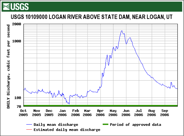
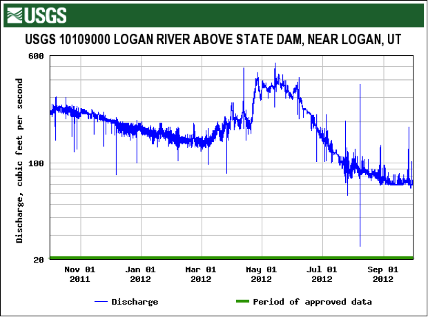
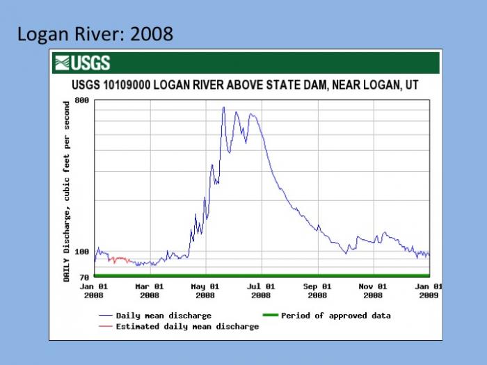
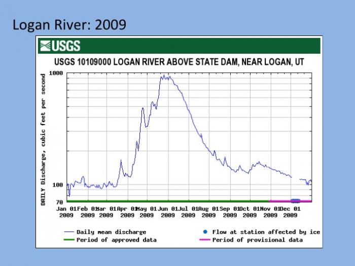
The Figure 4 shows example hydrographs from the Logan River, near Logan, Utah for two different water years (2006 and 2012). The water year begins October 1 and ends September 30. Hydrologists often prefer to conduct analyses based on the water year rather than the calendar year to facilitate comparison of incoming precipitation and outgoing streamflow, and specifically to ensure that snow delivered in October, November, or December is accounted for in the same time period that it is likely to melt, which may be in spring or summer of the following calendar year.
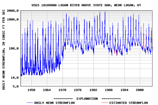
The Logan River hydrograph shows a long (about 5 month) prominent peak in discharge, primarily driven by snowmelt, with many other smaller peaks superimposed (from accelerated snowmelt during warm periods or rain events). The hydrograph of the Logan River over a 50 year time period (Figure 6) shows the prominent peak from snowmelt each year, but provides little information about the smaller scale variability that is visible on the annual timescale. Note the non-linear y-axis of the plots. Such axes can be useful for visualizing detail in both high and low flow conditions, whereas the detail in low flows would not be visible on (typical) linear axes. The apparent shift in low flows circa 1970 on the Logan River was caused by removal of a water diversion upstream from the gauge. Note that there is a considerable amount of ‘noise’ (i.e., variability) in streamflow over the past 50 years. This variability is not random, but rather has some ‘structure’ to it, some of which is visibly obvious (annual peaks) and other portions that can only be quantified using advanced analytical or statistical techniques, which are beyond the scope of this course, but currently represent a vibrant facet of hydrologic research.
Examples of Logan River Hydrographs 2008-2009
River Flow Regimes
River Flow Regimes
The temporal patterns of high and low flows are referred to collectively as a river’s flow regime. The flow regime plays a key role in regulating geomorphic processes that shape river channels and floodplains, ecological processes that govern the life history of aquatic organisms, and is a major determinant of the biodiversity found in river ecosystems. There are five components that characterize the flow regime:
- Magnitude: the total amount of flow at any given time
- Frequency: how often flow exceeds or is below a given magnitude
- Duration: how long flow exceeds or is below a given magnitude
- Predictability: regularity of occurrence of different flow events
- Rate of change or flashiness: how quickly flow changes from one magnitude to another
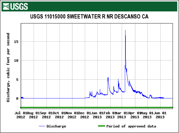
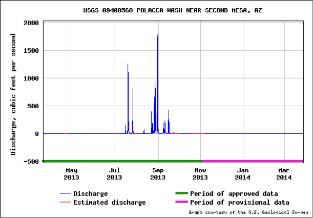
River in regions with similar climate, geology, and topography tend to have similar flow regimes. For example, rivers draining high mountains, such as the Logan River, tend to have relatively infrequent, high magnitude, long duration, and predictable flood events that have a slow rate of change (Figure 6 on the previous page). Rivers in many tropical climates have similar flow regime characteristics as mountain rivers, due to predictable rainy and dry seasons. In contrast, rivers in arid regions are often characterized by high magnitude, short duration floods of low predictability and high flashiness (e.g., Figure 11 on the next page).
Within regions of similar climate, local factors such as soil type, soil depth, vegetation cover, and watershed size influence the natural flow regime. For example, watersheds with deep, permeable soils will be able to absorb more precipitation than watersheds with thin, impermeable soils, and will thus tend to have less flashy floods of lower magnitude and longer duration. Large rivers tend to be less flashy than small streams, which respond more quickly to individual precipitation events. Thus, natural flow regimes can be somewhat variable between nearby watersheds. Also, although general patterns in flow regime can be determined from watershed characteristics, yearly variation in precipitation patterns means that many years of flow monitoring will be required to fully characterize the flow regime of individual rivers.
Temporary vs. Perennial Streams
Temporary vs. Perennial Streams
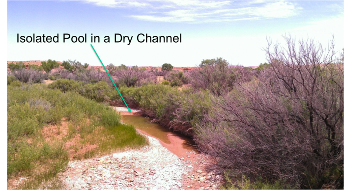
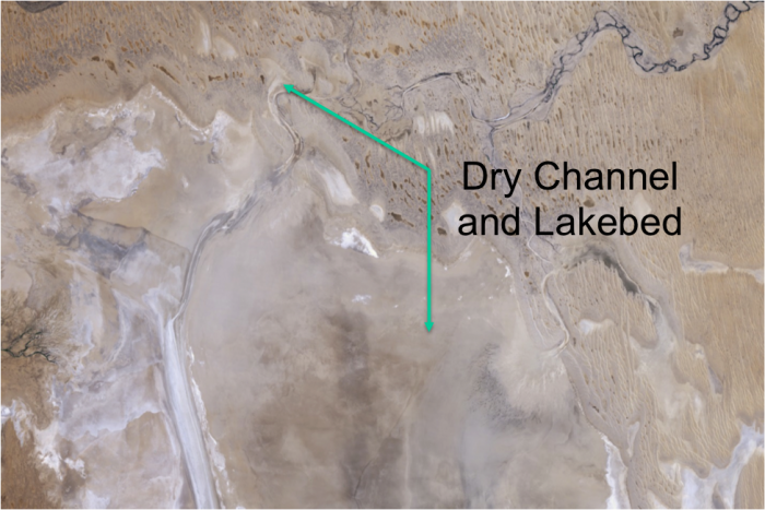
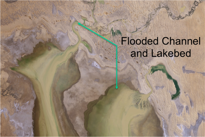
Most large rivers are perennial, meaning they maintain flow throughout the year. However, many headwater streams or streams in arid regions sometimes run dry. A stream is considered temporary if surface flow ceases during dry periods. Temporary streams are often classified further as intermittent and ephemeral. An intermittent stream becomes seasonally dry when the groundwater table drops below the elevation of the streambed during dry periods. A spatially intermittent stream may maintain flow over some sections or surface water in deep pools even during dry periods due to locally elevated water tables or perched aquifers. An ephemeral stream only flows in direct response to precipitation such as thunderstorms. Thus, the flow variability of an intermittent stream is much more predictable than in an ephemeral stream.
In many parts of the world, such as the desert southwest, temporary streams may comprise a majority of the river network, >80% in some areas. However, even in wet regions, temporary streams at the head of river networks can account for >50% of the total stream network. Thus, river networks can be considered dynamic systems, with total miles of surface flow expanding and contracting in response to precipitation events.
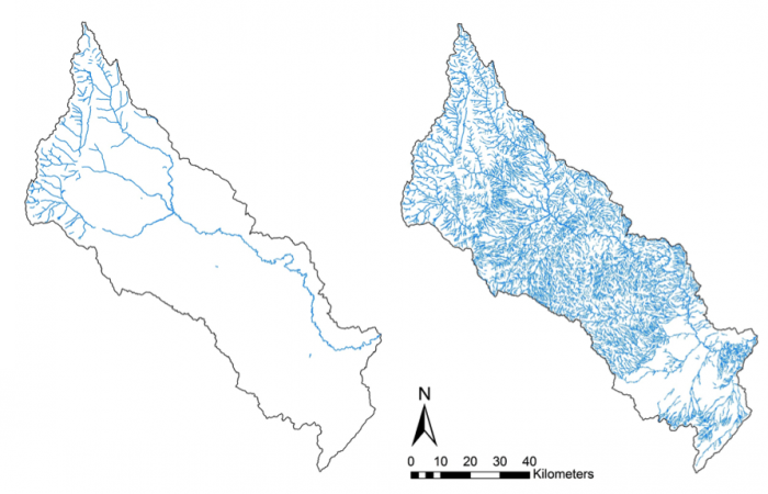
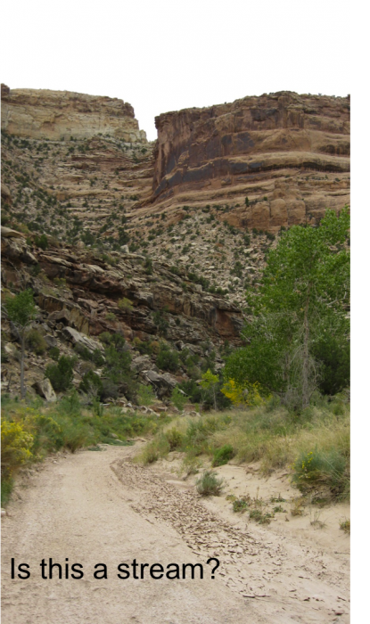
Why would we still call a channel that goes dry for much of the year a stream? In other words, how can we distinguish between a temporary stream and an upland terrestrial ecosystem? In short, a stream has characteristic hydrological, geomorphological, and ecological processes. However, as with many topics in environmental science, the distinction between stream channels and uplands and between perennial streams and temporary streams is often fuzzy and scale-dependent. Individual stream channels may hold water for decades and then become dry during exceptional droughts that occur infrequently (once every 50-100 years). Similarly, small gullies on hillsides may flow only a few days of the year and may transport sediment but not be resident to aquatic life. Are such systems part of the river network?
What is a Stream?
What is a Stream?
A channel is generally classified as a stream based on the occurrence of several processes including Hydrological Processes, Geomorphological Processes, and Ecological Processes.
Hydrological Process
Hydrological Process
Definition
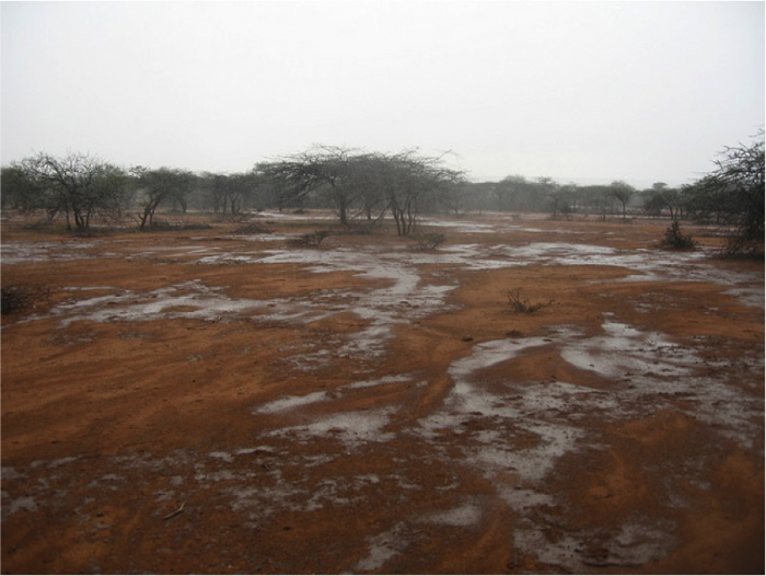
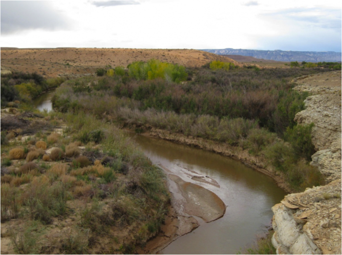
A proper stream generally consists of concentrated, channelized flow, even if it only carries water for a few days of the year. In contrast, an upland system may have surface water flow, but the flow is more akin to sheet flow and typically not concentrated into channels.
Geomorphological
Geomorphological
Definition
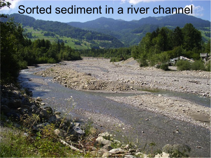
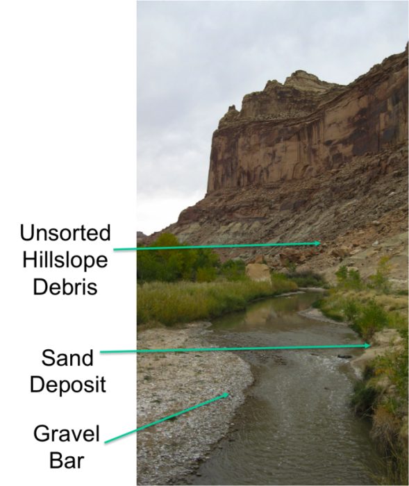
A stream channel is an area of rapid conveyance of sediment and dissolved constituents during periods of flow. However, not all sediment can be transported during all flows, and this provides a mechanism and particular pattern of sediment sorting that is a hallmark of stream channels not found in terrestrial systems.
Ecological Processes
Ecological Processes
Definition
A stream channel supports populations of aquatic organisms such as fish and insects. In contrast, upland systems do not provide even temporary habitat for aquatic organisms. Even when stream channels go dry on the surface, fish and other organisms can survive in isolated pools of water or in isolated areas of flow such as springs and perched aquifers.
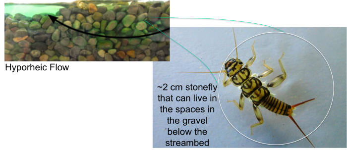
Many organisms can survive in the bed of a stream channel even if the surface is dry, due to hyporheic flow, which is water that flows in the sediments of a stream channel beneath the surface.
Even if aquatic organisms do not persist in stream channels year-round, temporary flooding can provide productive systems and isolation from predators, favorable for reproduction and development of young organisms, which can then migrate to perennial rivers as the stream dries.
Flow Duration Curve
Flow Duration Curve
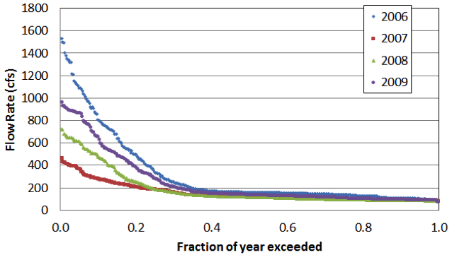
While it can be very informative to study hydrographs and the other flow metrics described above, often an important question often asked about rivers is ‘what percentage of time does flow exceed (or not exceed) a given value (e.g., 100 cfs)?’ It might be important to answer that question to determine the percentage of time when the flow is too low to support a particular fish species. Or it may be important to know what percentage of time the river exceeds a certain value known to cause flood damage. The proportion of time any given flow is exceeded can be determined by generating a flow duration curve. Figure 21 shows the flow duration curve for the hydrograph shown in Figure 21 (2006 water year) as well as the three subsequent years. You can immediately see that the mid and lower flows (exceeded about 40% (or 0.4) of the year) are relatively similar in each year, but the larger flows exhibit quite a bit of variability. In 2007 the highest flow of the year was only a bit over 400 cfs, while it was over 1500 cfs in 2006. The flow that was exceeded 20% of the time (0.2 on the x-axis) was approximately 450 cfs in 2005, but only 200 cfs in 2007.
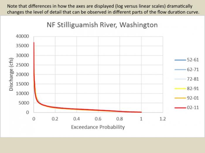
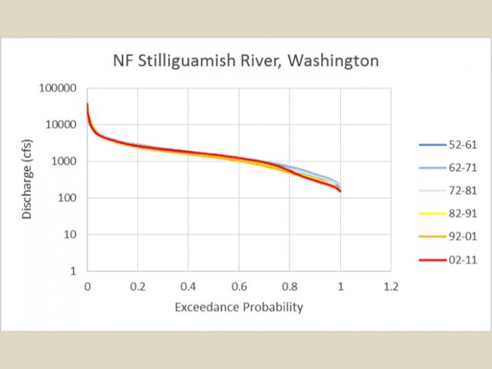
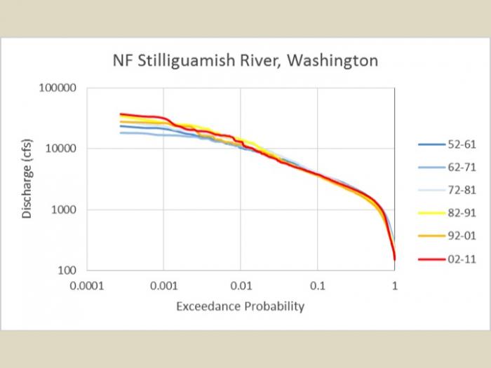
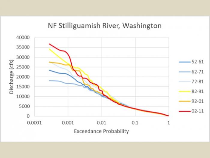
Note that this plot provides detailed information on different parts of the flow duration curve depending on whether you use linear or log scales for the x or y axes (see example from the Stilliguamish River, Washington below in Figures 22-25).
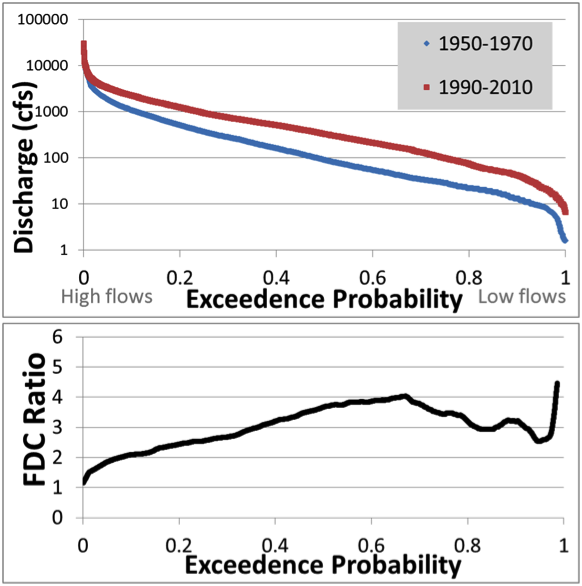
Flow duration curves can be made for a given river over two different time periods to illustrate if/how the range of flows has changed over time. For example, Figure 27 shows flow duration curves for the Le Sueur River in southern Minnesota for two different time periods (1950-1970 in blue, 1990-2010 in red). Note that in these plots the fraction of year exceeded is labeled as ‘exceedance probability’. These two terms are interchangeable, both being computed as:
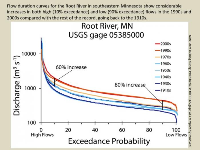
Where Ep is the exceedance probability or the fraction of the year that a given flow is exceeded, R is the rank, and n is the total number of values (365 if you are using daily-averaged flow values for a non-leap year). High flows (toward the left side of each plot) and low flows (toward the right side of each plot) appear not to have changed in the Elk and Whetstone rivers. In the Blue Earth River, low flows (exceeded more than 85% of the time) have not changed much, but mid-range and high flows all appear to have increased. In the Le Sueur River, the full range of flows appears to have increased. Note that the y-axis is plotted on a log scale, so even the modest difference between the two curves represents a significant increase in high flows (e.g., those that are only exceeded 5-10% of the time). The Root River, in southeastern Minnesota, has experienced significant increases in high and low flows within the past two decades, see example above.
Learning Checkpoint
1. What percentage of an average river network is made up of temporary streams:
(a) 0%
(b) 100%
(c) 10%
(d) 50%
ANSWER: d. 50%
2. What percentage of an average river network is made up of temporary streams:
(a) 0%
(b) 100%
(c) 10%
(d) 50%
ANSWER: b. 0.25
3. Given your answer to the previous question, how many days of the year was flow of the Logan River above 400 cfs in 2006?
(a) 37
(b) 91
(c) 256
(d) 329
ANSWER: b. 91
4. In Figure 21, what fraction of the year did flow of the Logan River exceed 400 cfs in 2007? Click to see Figure 21. [4]
(a) 0.01
(b) 0.1
(c) 0.9
(d) 0.99
ANSWER: a. 0.01
5. Given your answer to the previous question, how many days of the year was flow of the Logan River above 400 cfs in 2007?
(a) 4
(b) 37
(c) 329
(d) 361
ANSWER: a. 4
6. According to Figure 27, how much did the median (i.e., 50% exceedance) flow change in the Le Sueur River between the two time periods represented. Click to see Figure 27 [5]
(a) by a factor of 0.5
(b) by a factor of 2
(c) by a factor of 3.5
(d) by a factor of 10
ANSWER: c. by a factor of 3.5