Driving Forces for Groundwater Flow
Driving Forces for Groundwater Flow
The driving forces that control groundwater flow are a bit more complicated than those controlling flow in rivers and streams. As you learned in Module 3, surface water flows downhill due to gravity, and the flow direction is defined by the topography. Water flows downhill because gravity is a form of potential energy – and the water, or anything that falls or rolls downward – flows in response to differences in potential energy (from high to low).
In contrast to surface water, groundwater is separated from the atmosphere, and as a result, it can be under considerable pressure. Therefore, the potential energy that drives groundwater movement includes both pressure and gravity. In this section, you will learn about these driving forces, how we define them, and how they translate to the direction and rate of groundwater movement in the subsurface.
Potential Energy and Hydraulic Head
Potential Energy and Hydraulic Head
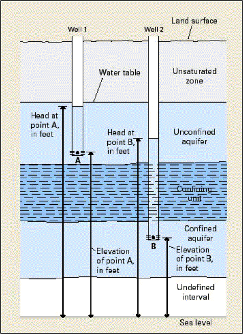
The flow of both surface water and groundwater is driven by differences in potential energy. In the case of surface water, flow occurs in response to differences in gravitational potential energy caused by elevation differences. In other words, water flows downhill, from high potential energy to low potential energy. In groundwater systems, things are a bit more interesting. Unlike surface water, which is in contact with the atmosphere and therefore rarely under pressure, water in groundwater systems is isolated from the land surface. This means that groundwater can also have potential energy associated with pressure. In extreme cases, water in confined aquifers may be under sufficient pressure to drive flow upward, against gravity. Artesian wells are one manifestation of this.
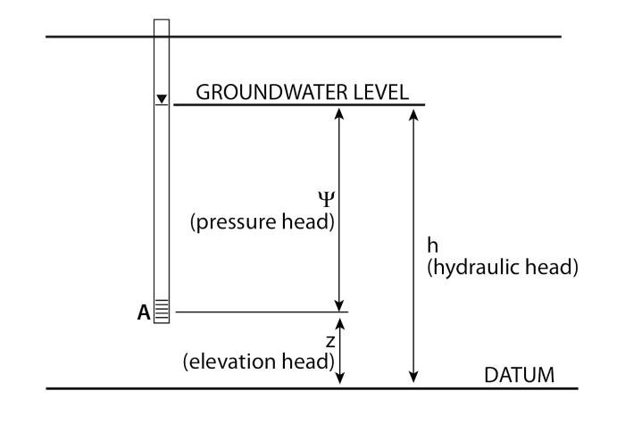
Fundamentally, groundwater and surface water are similar in that flow is in the “downhill” direction. But what does “downhill” mean in a groundwater system? To define the flow direction, we need to account for the two types of potential energy. Unfortunately, the potential energy of the water cannot be measured directly. However, we can measure a proxy for the potential energy by measuring the hydraulic head, or level to which water rises in a well (Figures 26 and 27). The hydraulic head combines two components: (1) potential energy contained by the water by virtue of its elevation above a reference datum, typically mean sea level; and (2) additional energy contributed by pressure. In a well, the value of hydraulic head represents the potential energy of the water at a particular point in three dimensions – at the depth where the well is open to the aquifer (Figures 26-27). This is analogous to a temperature reading taken at the tip of a thermometer, which provides a proxy for heat energy. Hydraulic head can be written as:
h = z + Ψ,
where z is the elevation energy, and Ψ is the pressure energy.
Click to expand to provide more information
Hydraulic Head and the Direction of Groundwater Flow
Hydraulic Head and the Direction of Groundwater Flow
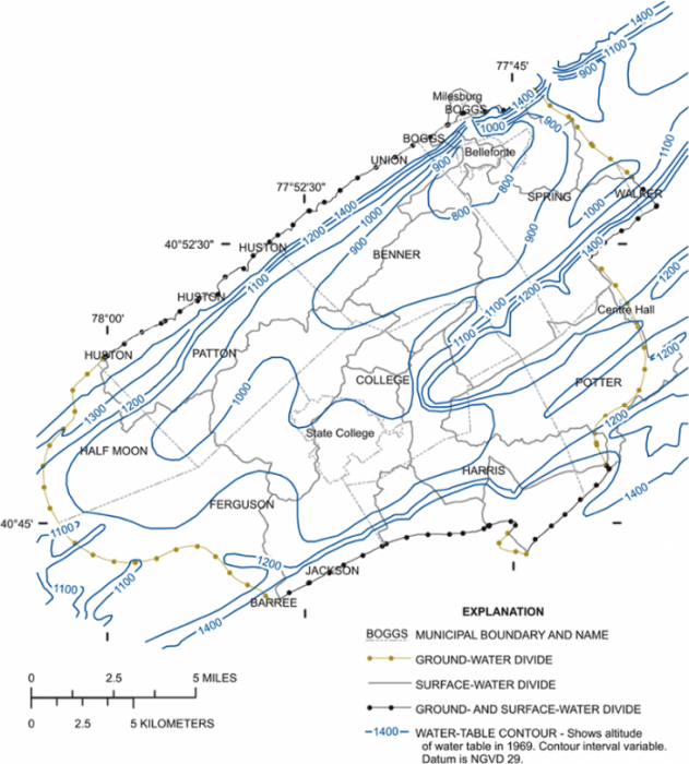
In order to define groundwater flow directions and rates through aquifers, individual measurements of hydraulic head are combined to generate contour maps of water level – or potential energy (Figure 29). These maps define the potentiometric surface, which is much like a topographic contour map but defines the distribution of potential energy in the groundwater system. Each contour, or equipotential, represents a line of equal hydraulic head.
To first approximation, groundwater flows down-gradient (from high to low hydraulic head). As is the case with surface water, or a ball rolling down a hill, the water flows in the direction of the steepest gradient, meaning that it flows perpendicular to equipotentials. There are exceptions to this – for example, if the hydraulic conductivity of the aquifer is much higher in one direction than another, or dominated by fractures with particular orientations, then these can redirect groundwater flow askew to the maximum gradient.
The potentiometric map also provides clues about the rate of groundwater flow. If you think back to Darcy material and our in-class activity from last week, you will recall that groundwater flow rate depends on the head gradient (i.e. the hydraulic gradient) and hydraulic conductivity. In a simple one-dimensional Darcy tube experiment, the head gradient is just the difference (h1-h2)/L. In two dimensions, the head gradient is defined by the slope of the potentiometric surface – just as the slope of the land surface is defined on a topographic map. The path that water takes in the aquifer, defined as a continuous line tracing the maximum gradient on a map of the potentiometric surface, is known as a flowline.
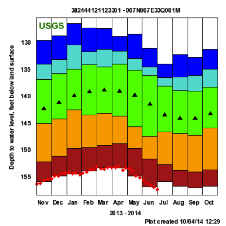
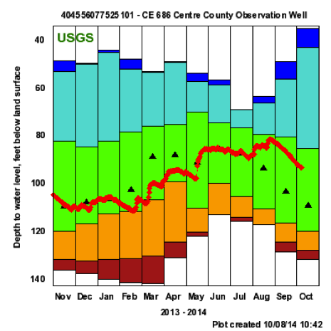
Well Hydrographs
Well Hydrographs
Just as river hydrographs are used to record and visualize variations in flow with time (as discussed in Module 4), a well hydrograph is a time series of hydraulic head recorded in a well. This provides information about the fluctuation of hydraulic head (equivalent to the water table in an unconfined aquifer), which reflects the combined effects of temporal variations in climate, recharge, and pumping (Figures 30-31). The U.S. Geological Survey maintains a database of active monitoring wells [1] in major aquifer systems across the United States. Hydrographs provide information about seasonal patterns that may be associated with pronounced wet and dry seasons typical of some regions (for example, Central CA), as well as long-term trends driven by climate change, decadal-scale climate patterns like el nino, prolonged groundwater extraction, or human-induced modifications to natural recharge. We’ll cover examples of the latter two processes in the next section of the module (Module 6.2: Water budgets).