Lesson 8: Not-So-Ordinary Earthquakes
Overview
This lesson will last one week. In it, we'll explore some things scientists have learned about how faults work that are new (since early 2000s) discoveries.
Objectives:
By the end of Lesson 8 you should be able to:
- Download, manipulate, and analyze publicly available earthquake catalog data from the Incorporated Research Institutions in Seismology (IRIS) and from the United States Geological Survey (USGS).
- Download, manipulate, and analyze publicly available geodetic data from UNAVCO.
- Calculate plate velocities and earthquake slip from geodetic data
What is due for Lesson 8?
Lesson 8 will take us one week to complete: 29 Jul - 4 Aug 2020.
The chart below provides an overview of the requirements for Lesson 8.
| Requirement | Submitted for Grading? | Due Date |
|---|---|---|
| Teaching/Learning Discussion III | Yes- this discussion will be part of your overall discussion grade | 12 Aug 2020 |
| Problem set: Spectrum of Fault Slip problem set | Yes - this exercise will be submitted to the "Slow Slip problem set" assignment in Canvas | 4 Aug 2020 |
Teaching and Learning III
Let's discuss the topics covered in Lessons 6 and 7, plus any other tidbits you've been dying to get off your chest all semester. Now's your chance!
Post to the Teaching/Learning 3 discussion board in Canvas. Don't be shy. This discussion is scheduled for this week plus the week devoted to the capstone project.
Measuring plate motion with geodesy
The sudden movements on faults that produce earthquakes are recorded by seismometers, but we know that all the plates on the surface of the Earth are in constant motion. Over the past ten or fifteen years, global positioning system satellite data has become an invaluable tool for measuring plate motion and strain accumulation across faults. This data is gathered by installing geodetic markers in the ground. Scientists then use GPS receivers at the sites of the markers to find out their exact locations from satellites. Over time, the position of the markers shift as the plate they are affixed to moves. The markers also move relative to each other; for example, markers on opposite sides of a fault may move closer together or further apart or be offset laterally as the years go by. This motion can be used to infer the strain rate in the crust. After several years of repeated measurements, the motion of the markers over the measurement time period is assessed. At active plate boundaries, such as along the San Andreas Fault on the West Coast of the United States, geodetic surveys have been used in concert with detailed records of seismicity to estimate stress buildup on faults and to predict seismic hazard. For example, a suite of geodetic markers may be placed around a fault of interest. After many measurements, the motion of the markers relative to each other can confirm the sense of motion on the fault, how fast the plates on either side of the fault are moving, and whether the fault itself is creeping or locked.
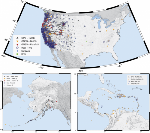
The Plate Boundary Observatory was a geodetic observatory designed to study the three-dimensional strain field resulting from deformation across the active boundary zone between the Pacific and North American plates in the western United States. The observatory consisted of arrays of Global Positioning System [1] (GPS) receivers and Strainmeters [2] (see map below for the locations of currently installed PBO instruments) which were be used to deduce the strain field on timescales of days to decades and geologic and paleoseismic investigations to examine the strain field over longer time scales.
The PBO was combined with some other networks in Central and South America in 2018 and is now called NOTA, Network of the Americas. You can read more about it UNAVCO's website [3].
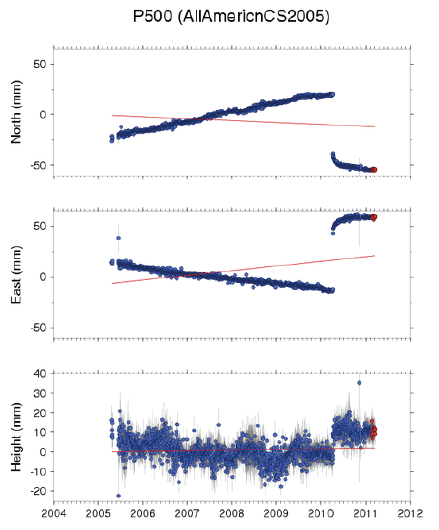
What does GPS time series data look like?
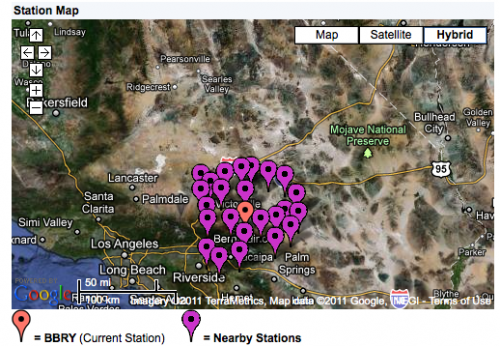
Let's walk through the signals recorded by a typical PBO geodetic station. I chose a station at random in Big Bear City, California, called BBRY. The map below shows a snapshot of the location of BBRY (the orange one) as well as a bunch of nearby stations (the purple ones).
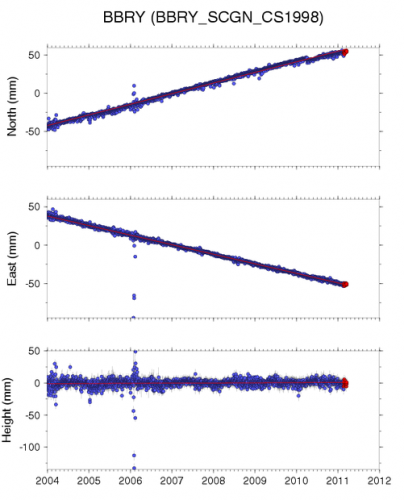
Typically, GPS stations record their position based on communicating with a satellite once per day or so. Below are plots of the three components of time series data recorded by BBRY since 2004. All three plots have time on the x axis. The top plot shows position in the north-south direction, the middle plot shows position in the east-west direction, and the bottom plot shows vertical position. When I look at these plots, I see that since 2004, BBRY has been moving steadily to the northwest and its vertical position is basically constant. How do I read this from the plots? Let's check it out together (pencast) [4]. You may also want to check out UNAVCO's reference guide [5] for reading GPS time series plots.
Calculate plate motion using GPS data
Determining plate motion: displacement
How far and in what direction did station BBRY move between since January 2004 and March 2011? This is a reasonable question to ask because it helps us determine strain rate in the crust.
The way to do it is:
- Observe each of the three components of the time series data and measure the displacement for each one. In the time series plots, each blue dot is a verified measurement, the red dots are the most recent measurement that probably have not yet been checked for accuracy, and the red line is a linear best fit line (done by a computer program) to the data.
- Then, add the three components of motion.
That's all! But there's a small wrinkle. The motion is happening in three-dimensional space. We need to use vector addition to get the right answer. This sounds fancy, but we just need to remember the Pythagorean theorem. Maybe you've only used this theorem to find the hypotenuse of a right triangle, but it works nicely in three dimensions, too:
north2 + east2 + vertical2 = total2
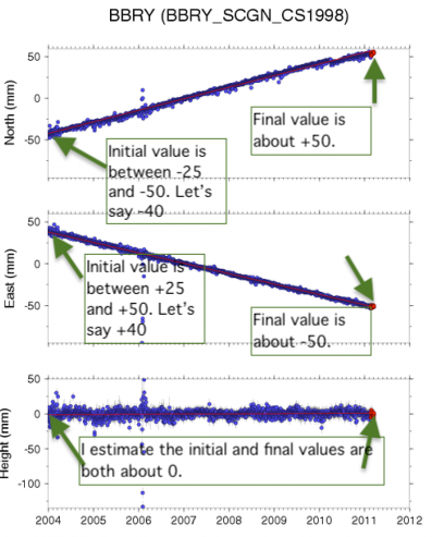
If you wanted greater accuracy, you should get the actual data for a station, instead of just visually estimating from a plot, but for our purposes here, estimation is going to be good enough. So let's do it. The north component has gone from -40mm to +50mm, for a total of 90mm north. The east component has gone from +40mm to -50mm for a total of 90mm west. (WEST! because negative East is West). The vertical component looks like it hasn't changed. Let's assume the vertical motion is zero, so neither up nor down over this time period.
We can use the Pythagorean theorem to get the answer:
902 + 902 +02 = total2
8100 + 8100 + 0 = total2
16200 = total2
sqrt(16200) = total
127.28mm northwest is my answer. I probably shouldn't keep two places past the decimal given how cavalier I was about my initial observations from the plot, so let's round to a whole number. BBRY moved about 128 mm northwest between January 2004 and March 2011.
Determining plate motion: velocity
What was the average velocity of BBRY between January 2004 and March 2011? We already have all the information we need to make this calculation.
velocity = distance / time
We know the distance because we just calculated that. What about time? Here's something fun about geodesy: The convention is to divide up a year into 10 equal parts instead of using months, or days. Months are all different lengths, so this way of doing things makes calculations easier. See how each year on the x axis has 10 little tick marks on the plot of BBRY that we've been looking at. What time span is covered by the data in the plot? It goes from the beginning of 2004 up to about the second tick mark after the beginning of 2011. So let's call that 8.2 years.
velocity = 128mm / 8.2 years
velocity = 15.61mm/year
Once again I don't think we should keep so many digits after the decimal. We can't justify that level of precision. Let's round and say BBRY has moved at a rate of about 16 mm/year northwest. Now we could look up what an "accepted value" is for how fast various plates move and compare our calculations to those. We'd need to look at a map and make sure we know which plate BBRY is sitting on.
This kind of calculation verifies the calculations you did back in Lesson 3 with Fred Vine's data from the 1960's, which is cool!!
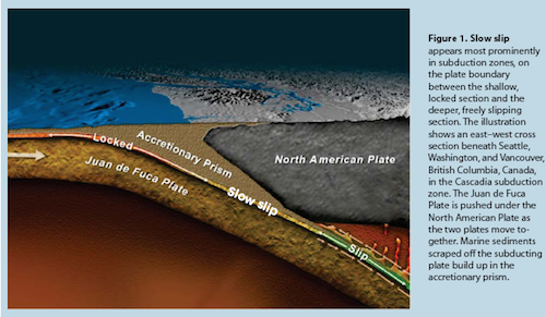
The Secret Lives of Subduction Zones
Cool things happen at subduction zones. In Lesson 6 we explored volcanoes that happen at these plate boundaries. Now let's explore how those plate boundaries move mechanically to generate earthquakes, and a relatively newly discovered phenomenon called "slow slip." First of all, let's remember what a subduction zone looks like, and what kinds of instruments we use to figure out what it's up to.
Quiz Yourself Review!
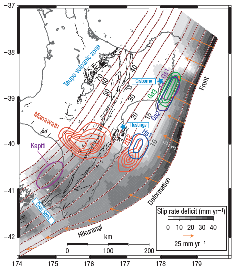
Let's review some things from Lesson 6 by looking at the drawing of the Cascadia subduction zone above.
Where are the Cascade Range volcanoes on the upper plate? Where does that correspond to on the lower plate? What kind of volcanoes are they? What kind of melting produces these volcanoes and how is it depicted in the cartoon?
Think about it and then watch my explanation as a screencas [6]t. You can also read a transcript of my quick Lesson 6 review [7].
Subduction zone mechanics: standard textbook vs. what we know now
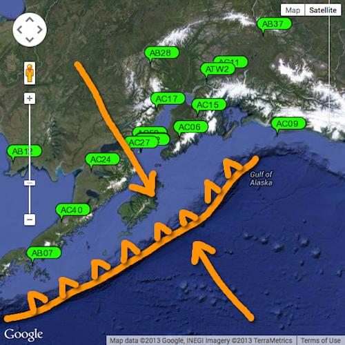
Below is a “textbook” depiction of a subduction zone [8] and associated plate movement. This is a map of southern Alaska. In an introductory class or typical textbook, we’d probably draw arrows right on the plate boundary (trench) showing the two plates converging, like I did in this map. The teeth are on the upper plate. The Pacific Plate is heading northwest and diving under Alaska. The green bubbles are GPS station locations. The orange arrows show the direction of motion of the two converging plates.
Geodetic data from instruments near plate boundaries tell us that the image above is an oversimplification. In a subduction zone capable of sustaining great earthquakes, the upper plate and lower plate are locked together for some distance inboard of the trench. Therefore GPS stations on the upper plate near the plate boundary will record motion consistent with the direction of the lower plate. In fact, geodetic data can be used to infer the location of the locked section (see figure below).
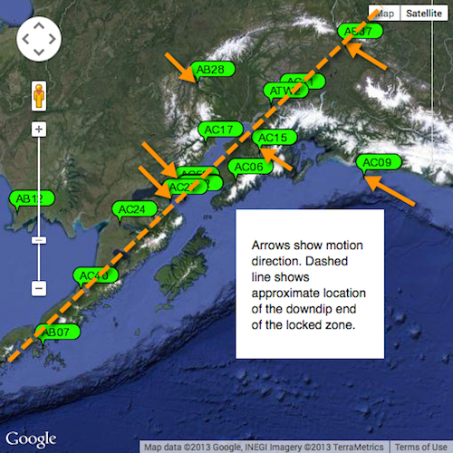
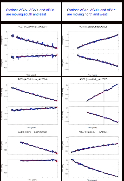
The point here is to see, via GPS, how the portion of the upper plate directly on top of the locked zone is dragged along in the direction of subduction because the plates are locked together. Green bubbles point to PBO stations. GPS stations on top of the locked zone show motion in the direction of the lower plate (northwest). GPS stations on top of the freely slipping zone show movement in the direction of the upper plate (southeast). We can infer where the locked zone ends by knowing the angle of subduction and by looking to see where the GPS stations record direction of motion consistent with the upper plate’s macro-motion.
The GPS time series plots show motion south and east for stations AC27, AC59, and AB28. Those three stations are all far enough inboard on the upper plate that they are not over the locked zone. The GPS time series plots show motion north and west for stations AC15, AC09, and AB37. Those three stations are closer to the plate boundary and are over the locked zone. They are moving in the direction of the lower plate.
What does an earthquake look like in a GPS time series?
A GPS station normally records its position once per day. An earthquake only takes seconds to minutes to happen so a GPS station doesn't record all the details, like the arrival of P waves and S waves and things like that. It only records its own position. If the earthquake is big enough and nearby enough, GPS will show a sudden jump in the direction of earthquake slip. Let's check that out with an example.
This is a station near the border of Baja CA and the US. It shows background plate motion to the northwest, then a sudden jump to the southeast. Sudden big jumps in geodetic data (that are not data dropouts!) are earthquakes. Most geodetic data is recorded daily but earthquakes take way less than a day to slip, so there is a sudden gap on the y axis. (A gap in x denotes a data dropout due to an equipment problem or something like that)
Slow Slip Events
For a long time we were all pretty happy with the idea that the life of a subduction zone involved a cycle of building up stress and having an earthquake that released the stress, then starting over again. But it turns out there's more going on.
Slow slip events have only been discovered in the last 10 or 15 years! They occur between the locked section and the freely slipping section of a subduction zone. Some people refer to the “locked section” as the seismogenic zone. If you are going to have a great subduction zone earthquake, such as Alaska 1964, or Chile 1960, or Tohoku-Oki 2011, this is the zone where it initiates and ruptures. The freely slipping section is the part of the downgoing plate that is too deep to be touching the other plate. It's the part that is hanging down into the mantle. In most subduction zones there is a region between the locked and the freely slipping parts, and that is where slow slip happens. It is usually at about 30-70 km depth.
Slow slip events do not generate seismic waves, so seismometers do not record them. GPS stations can, though! What does one look like? Let's check that out.
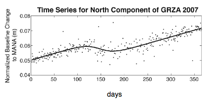
This figure was modified from Outerbridge et al., 2010 and depicts GPS time series data that was recorded in Costa Rica in 2007. It shows a slow slip event that took place between about day 125 and day 175 on this plot. Why do we call this a slow slip event? It is too fast to be the usual plate rate, and it is also in the opposite direction. It is way too slow for an earthquake because remember in the earlier GPS time series from Baja that an earthquake basically looks like a sudden jump that happens all at once, not something that takes 50 days to happen.
Check that you can read this plot!
What is the background plate direction and rate? What is the duration, direction, and rate of the SSE? Try it yourself and then click below to see my answers:
My answers to the posed questions.
The background plate rate (eyeballing here) looks like about 0.01 m per 100 days to the north, which is equivalent to 3.7 cm/year. That's a reasonable ballpark number. Note that we are only looking at the north component here so we can't say anything about whether it's east/west or up/down. The SSE begins around day 125 and lasts about 50 days. During that time this station moved about .005m south. From about day 175 until the end of 2007, this station was back to its usual plate rate.
Quick quiz to check yourself
An SSE involves slip in the same direction an earthquake would move, or in the same direction as background plate rate? Or are those two directions the same?
Answer to the quick quiz
An SSE involves slip in the same direction an earthquake would move, which is opposite the ordinary direction of this station because this station is on the part of the upper plate locked to downgoing plate. One way to remember this is that GPS stations are land-based. Land is always on the upper plate side of a subduction zone. So, GPS stations at subduction zones are measuring the position of stations on the upper plate. Stations over the locked zone will show you the sense of motion of the lower zone. Stations farther away from the plate boundary in the interior of the upper plate record the motion of the upper plate. Mechanically, the upper plate over top of the locked zone is getting scrunched during interseismic periods. During an earthquake it suddenly unscrunches. A slow slip event is a really slow unscrunching that seismometers can't hear.
Slow Slip Events: More details
Rupture characteristics of slow slip events
- They slip faster than the plate speed but slower than an earthquake. Millimeters per week is a good ballpark estimate of the speed.
- The ones measured so far slip as much as a large-magnitude earthquake but take a lot longer to accomplish that slip. That's why they are called "slow slip events."
- They are not detectable by seismometers due to the long rise time and slow rupture velocity. We use Global Positioning System data to measure them.
For example, the rise time for an earthquake is often negligible compared to the rupture duration, but for a slow slip event, the rise time can be a significant fraction of the overall time of rupture.

Rise time? What's rise time?
The rise time is how long it takes an earthquake to go from zero to its seismic rupture velocity. Generally speaking, earthquake rise times are fast compared to how long the earthquake lasts. Another interesting thing about earthquake rise times is that they are about the same regardless of the final size of the earthquake. The rise time of a magnitude 5 and a magnitude 8 are about the same. The difference is that a magnitude 8 lasts longer and a bigger chunk of ground is involved in the earthquake. For a slow slip event, the rise times are incredibly long and the event never does get up to a seismic speed at all. Since the motion is all so smooth and slow, seismic waves aren't generated. That's why we have to use GPS instead of seismometers to measure slow slip events. See my screencast for a sketch explaining rise time [9]. Click here for a close-captioned version of the rise-time sketch [10].
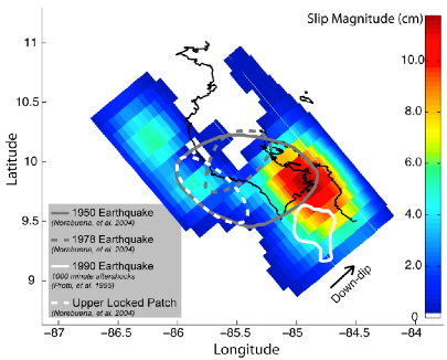
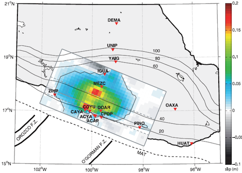
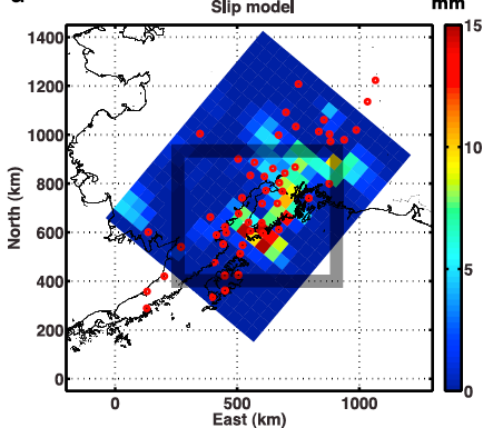
Where have slow slip events been found?
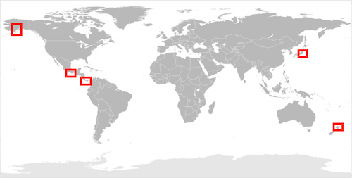
The figures below are reproduced from published papers that describe slow slip events detected in New Zealand, Nicaragua, Mexico, and Alaska. Their locations in the grand scheme of the world are shown with rectangles on the world map above, except Japan is missing from the detailed maps below. All the slow slip events shown here have two main things in common:
- Long duration compared to an earthquake (days to months instead of seconds to minutes), and
- Cumulative slip equivalent to 6.9-7.5 moment magnitude.
Spectrum of Fault Slip problem set
Note for Fall 2017
The problem set is a pdf file in CANVAS in the Lesson 7 module called "SSEProbSet.docx"
Download it, create your own word processing document with your answers, then
Turn it in to the Canvas assignment called L7-Slow slip problem set
Bibliography and Additional Resources
Bibliography
Schwartz, S. Y., and J. M. Rokosky (2007), Slow slip events and seismic tremor at circum-pacific subduction zones, Rev. Geophys. 45, RG3004, doi:10.1029/2006RG000208
Radiguet, M., F. Cotton, M. Vergnolle, M. Campillo, B. Valette, V. Kostoglodov and N. Cotte (2011), Spatial and temporal evolution of a long term slow slip event: the 2006 Guerrero Slow Slip Event, Geophys. J. Int., 184, 816–828, doi: 10.1111/j.1365-246X.2010.04866.x
Outerbridge, K. C., T. H. Dixon, S. Y. Schwartz, J. I. Walter, M. Protti, V. Gonzalez, J. Biggs, M. Thorwart, and W. Rabbel (2010), A tremor and slip event on the Cocos‐Caribbean subduction zone as measured by a global positioning system (GPS) and seismic network on the Nicoya Peninsula, Costa Rica, J. Geophys. Res., 115, B10408, doi:10.1029/2009JB006845
Wei, M., J. J. McGuire, and E. Richardson (2012), A slow slip event in the south central Alaska Subduction Zone and related seismicity anomaly, Geophys. Res. Lett., 39, L15309, doi:10.1029/2012GL052351
McCaffrey, R., L. M. Wallace and J. Beavan (2008) Slow slip and frictional transition at low temperature at the Hikurangi subduction zone, Nature Geoscience, 1, 316-320, doi:10.1038/ngeo178
Vidale, J.E. and H. Houston (2012), Slow slip: A new kind of earthquake, Phys. Today 65, 38, doi: 10.1063/PT.3.1399
Here are a few more books that discuss the links between archaeology and earthquakes.
de Boer, J. Z. & Sanders, D. T. (2007). Earthquakes in Human History: The Far-Reaching Effects of Seismic Disruptions. Princeton University Press, p. 304.
Kovach, R. L. (2004). Early Earthquakes of the Americas. Cambridge University Press, p. 280.
Nur, A. & Burgess, D. (2008). Apocalypse: Earthquakes, Archaeology, and the Wrath of God. Princeton University Press, p. 324.
Here are other articles relevant to this lesson.
Showstack, Randy. (2011). Scientists Examine Challenges and Lessons From Japan’s Earthquake and Tsunami, Eos 92, p. 97-99.
Tell us about it!
Have another reading or Web site on these topics that you have found useful? Share it in the next Teaching/Learning Discussion!