Lessons
Lesson 1
Lesson 1 Introduction
Did you glance at the Course Orientation?
Before you begin Lesson 1, it might be helpful to check out the Course Orientation [1].
About Lesson 1
In this lesson, you will begin a trek toward understanding the significance of water on Earth and its importance to a host of unique features on your home planet. You will also apply the scientific method along the way, think about how hypotheses are best evaluated, and get a chance to hone your skills of critical reading. Reading scientific articles and papers in a critical way is an invaluable skill. You will be doing this with your own students' work as well as with the published literature. Not everything you read, even in the scientific literature, is correct, or even well-reasoned. In Earth science, well-reasoned speculation is acceptable, as long as it is identified as such. Thus, scientific articles should present one or more clear, identifiable hypotheses and should evaluate those hypotheses using data collected for that purpose, presented in the paper along with other supporting information.
With the proliferation of "self publishing" on the Web, one can find all sorts of "bad science." How do we promote the "critical thinking and reading" skill to our students to allow them to sort the wheat from the chaff? Practice, of course! We will ask you to read selected articles, discuss them with the class, and provide data plots that support your views and points. We will also ask you to translate that science-speak into a product that is interesting and accessible to the lay person. Let's dive in!
What will we learn in Lesson 1?
By the end of Lesson 1, you should be able to:
- Explain the Scientific Method and the concept of Multiple Working Hypotheses
- More critically read and evaluate scientific papers
- Communicate complex scientific arguments to nonscientists
- Plot and analyze data
- Explain current thinking about the origin of water on Earth
- Explain the Goldilocks principle of life on Earth
- Explain the importance of water oceans to the evolution and continuity of life on Earth
What is due for Lesson 1?
The chart below provides an overview of the requirements for Lesson 1. For assignment details, refer to the lesson page noted.
| REQUIREMENT | LOCATION | SUBMITTED FOR GRADING? |
|---|---|---|
| Activity 1: Quantification and Plot Analysis (1) | See "Activity 1" in Lesson 1 menu | Yes - Your discussion board participation counts toward your overall class participation grade [participation spanning 18 May -2 Jun 2020] |
| Activity 2: Critically Reading Scientific Literature and the Scientific Method | See "Activity 2" in Lesson 1 menu | Yes - Submitted to "Lesson 1, Activity 2" in Canvas Assignments by 2 Jun 2020 |
Questions?
If you have general questions, please post them to our Questions discussion forum, which is linked under the Discussions link in Canvas.
Venus, Earth, & Mars
The Habitable Zone and Earth’s Oceans
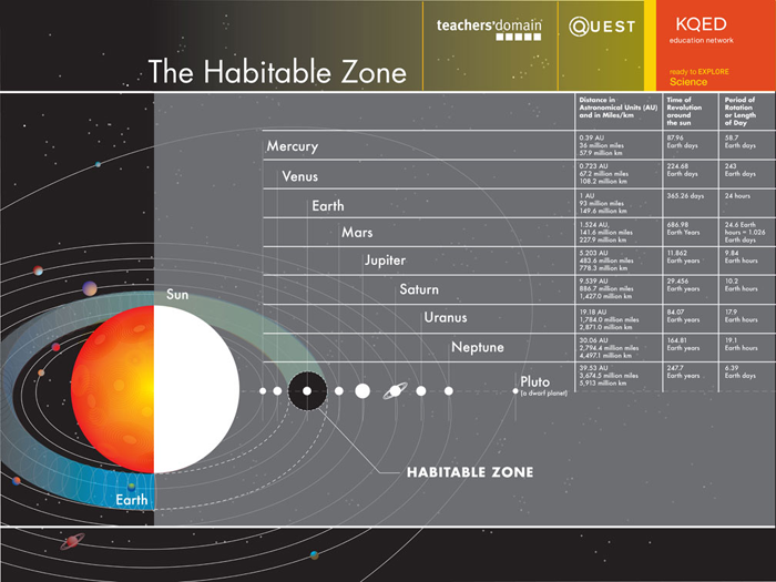
| Planet | Distance in Astronomical Units (AU) and in Miles/km | Time of Revolution around the sun | Period of Rotation or Length of Day |
|---|---|---|---|
| Mercury |
0.39 AU 36 million miles 57.9 million km |
87.96 Earth days | 58.7 Earth days |
| Venus |
0.723 AU 67.2 million miles 108.2 million km |
224.68 Earth days | 243 Earth days |
| Earth (Habitable Zone) |
1 AU 93 million miles 149.6 million km |
365.26 days | 24 hours |
| Mars |
1.524 AU 141.6 million miles 227.9 million km |
686.98 Earth Years | 24.6 Earth Hours - 1.026 Earth days |
| Jupiter |
5.203 AU 483.6 million miles 778.3 million km |
11.862 Earth years | 9.84 Earth hours |
| Saturn |
9.539 AU 886.7 million miles 1,427 million km |
29.456 Earth years | 10.2 Earth hours |
| Uranus |
19.18 AU 1,784.0 million miles 2,871.0 million km |
84.07 Earth years | 17.9 Earth hours |
| Neptune |
30.06 AU 2,794.4 million miles 4,497.1 million km |
164.81 Earth years | 19.1 Earth hours |
| Pluto (a dwarf planet) |
39.53 AU 3,674.5 million miles 5,913 million km |
247.7 Earth years | 6.39 Earth days |
Reading assignment
In our Astrobiology Research Center at Penn State, there is a room called “The Habitable Zone.” This whimsical name is a reference to a concept that has developed in the search for life on other planets. Of course, in “The Habitable Zone” room, there are comfortable couches, a coffee pot, computer connections and large screens for projection of computer images or teleconferences—all the ingredients for encouraging development of scientific intercourse, the lifeblood of the Astrobiology Research Center. A zone of habitability for life within a solar system has certain requirements too, including an optimal distance from a sun, optimal planet size and gravity, perhaps a magnetic field, and even the presence of a planet of large mass somewhere else in the solar system, among other characteristics. Some scientists speak of the “Goldilock’s Principle” for which everything needed to be “just right” for life to originate and prosper on Earth. We will explore this principle below, and you will need to discover what parameters are potentially important and why?
Question 1: What are the essential elements of a “habitable zone” for life and why is each important?
Not too long ago, we were pretty sure that Earth is the only planet in our solar system that has water present in all three phases on its surface. Quite a lot has changed in the past three or four years, with recent discoveries of liquid water on Europa, Mars and other bodies. Much of this is still very recent and uncertain, which makes it both exciting and also a nice example of science in action! For the Earth, oceans occupy about 71% of the surface area. Recent work suggests the presence of water oceans on Earth shortly after its formation (4.6 x 10⁹ years ago), as early as 4.3 to 4.4 x 10⁹ years ago. But from where did this water come? And why is there not abundant water on other planets today? Yes, we have good evidence for water in the subsurface on Mars, and water is a component of the Martian polar ice cap. Some scientists have suggested that water was once much more abundant on Mars’ surface—even forming large oceans.
Question 2: From where could Earth’s water have originated and what is the evidence in support of the origin(s)?
We don’t really have a definitive answer to this question at this time. Assuming that Earth and other planets accreted from a pre-existing solar nebula, possible sources of water on Earth could include capture of solar nebula gas (including volatile water vapor), adsorption of water from gas onto grains during accretion of these planets, accumulation and trapping of hydrous (water-bearing) minerals forming in the inner solar system or falling in from the asteroid belt, and impacts with comets and water-bearing meteors. Theories of the origin of water run the gamut from suggesting that all Earth’s water accumulated early in its history and, through various processes, was pooled into its vast surface oceans, to those that suggest importance for later water accumulation by repeated impacts of extraterrestrial objects. To be sure, Earth’s early accretion was a violent episode characterized by many impacts of “planetesimals,” from dust particles to objects as large as one tenth to one third of the mass of the accreting planet. Impacts ultimately provided sufficient energy to melt much of the earliest Earth, producing one or more “magma” (molten rock) oceans. At least one massive impact ejected material into Earth orbit, and this material subsequently accreted to form Earth’s Moon. We will revisit the Moon (at least in a virtual sense) and its significance to the oceans later in this course. Intense bombardment, referred to as the “late heavy bombardment”, ended about 3.9 x 10⁹ years ago. Evidence for this includes the large lunar mare (huge basins) produced by these large impacts.
Ocean Origins
The mass of Earth’s oceans is about 1.4 x 10²¹ kg. (How do we know this? See Activity 1, problem 1). But there appears to be far more water in Earth’s interior, something between 10 and 50 oceans' worth. It is likely that most of this water accreted within the Earth early in its history and that, in steady-state, some 5 to 10% remains on the surface in the ocean-atmosphere system. Although some evidence supports water delivery by later cometary or meteoritic (asteroidal) impacts, it is likely that surface water was accreted early and outgassed from within the Earth. Nonetheless, some new observations of comets (comet LINEAR) provide new support for cometary origins of water on planets in the inner solar system.
Want to learn more?
See "A Taste for Comet Water. [3]"
Question 3: Why are there oceans on Earth and not now on Mars or Venus?
Those two planets also likely accreted much water during their formation as well as having been bombarded by comets just as the Earth was.
Question 4: Why is liquid water on the surface of a planet important?
In a poll of the readers of Astrobiology Magazine, a scientific journal, 41% rated liquid water as the key factor needed to make a planet habitable, followed by a combination of all other candidate elements [nutrient, water, oxygen, ozone, photosynthetic sources like sunlight, and carbon dioxide].
Want to learn more?
See this collection of recent papers [4]. Start with the Introduction by J. Grotzinger [5]
Also see "Life's Little Essential [6]" by Peter Tyson.
Coevolution of Oceans & Life
Reading Assignment
For background in this section you will need to read two articles:
So, the "Goldilock's Principle" postulates that everything was "just right" on Earth for life to originate and prosper. Did water play a role? Make a list of all the ways that water could be important to the evolution and continuity of life on Earth (think broadly). For example, if Venus and Mars once had water, and even oceans, why do they not now have them? Clearly, if life arose in the presence of water, that water would have to persist in order to sustain life. Could life have evolved on Mars? Where would you look for life on Mars today?
One of the key constraints on the accumulation of oceans at the Earth's surface and the origin and survival of the earliest life on Earth is the size and frequency of objects that impacted the Earth. Lunine (2006) summarizes the impact history on Earth (largely inferred from the preserved record of impacts on Earth's Moon; why not directly from the earthly record?). Note that in the first 0.3 billion years (4.5-4.2 Ga) after Earth's accretion, the frequency and size of impactors was such that multiple "sterilizing" impacts occurred. In addition, these impacts probably "blew away" any oceans that may have accreted early and created a "steam" atmosphere. Certainly, some water was lost from Earth's surface to space. Fortunately, sufficient water existed either through accretion or continued addition by comets and asteroids (section 1) that oceans could again accumulate on Earth's surface. But life could have originated multiple times and been erased from Earth's surface by these large impacts. However, some models suggest that some life might have survived if it had evolved in higher-temperature environments, such as hot springs systems. In contrast, Venus and Mars somehow lost much of their water (and/or were initially endowed with much less than Earth?) during their early history, leaving Earth in the Goldilocks zone, and, perhaps, prohibiting an origination of life and/or continuity of life at their surface.
There is some evidence (what is it? See Lunine, 2006) for free water near Earth's surface as early as 4.4 Ga (the earliest known rocks extant on Earth) and fairly definitive evidence in rocks for large bodies of water (oceans?) by 3.6 Ga. Life may have arisen at that time, and there is reasonably strong evidence from structures and cellular features preserved in rocks that there were widespread mats of bacteria in shallow marine environments by about 3.3 Ga (Lesson 3 will entertain some hypotheses regarding the chemical composition of seawater). However, it took until nearly 0.54 Ga for multicellular marine animals to evolve. There is much speculation regarding the origin of life and why evolution took "so long" to allow more complex animals to exist. Little or no oxygen in the early atmosphere and oceans may have been a limiting factor, but there is disagreement regarding when the atmosphere-ocean system became "oxygenated." Available data indicate that some oxygen may have persisted in the atmosphere after 2.4 Ga, but more limited data may support an earlier timing for the "rise of oxygen." Note that oxygen can be considered a toxin to organisms that evolved in oxygen-deficient environments. Microbial organisms that once lived at the ocean surface would have been forced to seek refuge in oxygen-depleted environments below the seafloor when the oceans became oxygenated. Much work on this topic is going on in the Penn State Astrobiology Research Center as you read this.
Activity 1: Plot, Post, and Discuss
Activity 1: Quantitation and Plot Analysis (1)
Directions
Back of the envelope (BOTE) calculations are often useful to provide a perspective on the relative importance of a process or system mass balance (inputs vs. outputs). At times BOTE calculations are useful just to give one an idea how to approach a problem and to understand the relationships among the key parameters, and, perhaps, which ones need to be more precisely known. Scientists and others use plots to convey data relationships that are viewed as meaningful—perhaps to examine possible patterns or correlations that can provide insights into cause and effect.
We will use both in this course to help elucidate key ocean system details. So let's practice a bit. The exercise will also let you practice with scientific notation and unit analysis.
Start: A BOTE calculation (it's simple, but let's step through it).
Question: What is the mass of water in Earth's oceans? How would you go about determining this from some basic information? In other words, what values/parameters do you need?
Digression about mass, density, and volume
mass [m] is the amount of material that occupies a given volume. We will use SI units, so we'll talk about mass in kilograms (kg).
If you want to write the English sentence, "mass is the amount of material that occupies a given volume" as a math equation, you can write . Substitute the common symbols for mass, volume, and density, and you can write it as m=Vρ. Density is commonly the Greek lowercase rho.
Let's just check if this makes sense or not: mass is in kilograms (kg), volume is in meters cubed (m3), and density given in mass per volume, or kilograms per meter cubed, kg/m3. So if we substitute the units for the symbols in the m=Vρ equation we get kg = m3 * kg/m3. This is good news because some little algebraic manipulation shows we have the same units on both sides of the equals sign.
Back to our original problem: mass of the ocean
To obtain the mass of ocean water, we want to know the volume of the ocean and the density of seawater because volume multiplied by density gives us mass. What's the volume of the ocean? We need to find out the area of the ocean and its average depth to calculate its volume. And then we can look up a value for the average density of seawater. These numbers are known reasonably well and we can look them up in any oceanography textbook. Also I trust most internet search engines for "general knowledge" like this, so go ahead.
Note: we will often use several forms of scientific notation: 3.62 x 10¹⁴, or 3.62e14 or even 362 x 1012
Here are my numbers below, go ahead and look this up if you want to
Areaocean=3.62e14 m2 and average depth ~ 3800 m, so (you do the math)...
Vocean=1.375 x 10¹⁸ m3. Agreed?
The average seawater density is about 1037 kg/m3, therefore we have massseawater= 1.375e18 m3 x 1037 kg/m3 =1.426e21 kg. That's about 1.4e18 tons of seawater ( a metric ton=103 kg). Everybody see how we get here (and how to manipulate exponents and units)?
-
Part 1: A BOTE calculation for you to do.
- Question: What is the mass of water in Earth's interior? How would you estimate this? What values would you need (there might be several ways to do this)?
- Give it a try and post your answer in the "Lesson 1, Activity 1" discussion forum in Canvas. Engage your classmates in discussing final calculations and critical values.
-
Part 2: Plotting and Analysis (use your favorite plotting program, but produce an attractive plot with appropriate labeling).
- Find data (on the Web or in an oceanographic textbook, provide source) for the proportional distribution of water depths (area of the seafloor in each depth-range bin) for at least 13 depth bins (Hint: start with 0-200m, 200-1000m, then intervals of 1000m to maximum depth of the ocean). This may be hard to find. If you run into trouble you can use this source: Hypsometry of Ocean Basin Provinces, Menard and Smith, 1966 [9] This short article may also be of interest The Volume of Earth’s Ocean, Charette and Smith 2010, [10]
- Plot the distribution of depths as a function of the percentage of total ocean area (must sum to 100% of course). You now have what is termed a hypsometric curve for the oceans. Post this plot in the "Lesson 1, Activity 1" discussion forum in Canvas. You must figure out how to attach your plot in your post. I would suggest that you first save it as .jpg or .png or some other simple/small-file-size format. Make sure that your plot is high quality: both axes should have clear labels with units and the lines/symbols should be clear. For example, look at the plot on page 19 on this article, The Oceans, Their Physics, Chemistry, and General Biology [11]. It's a great example.
- Discuss how such a curve could provide insights into how the ocean basins formed. Why are some depth intervals such a large proportion of the ocean area? How else might a hypsometric curve be useful?
-
Part 3: Read the postings by other EARTH 540 students. Respond to at least one other posting in each part. You may ask for clarification, ask a follow-up question, expand on what has already been said, etc.
Submitting your work
- Enter the "Lesson 1, Activity 1" discussion forum in Canvas
- Reply to my starter posts for parts 1 and 2 and reply to some of your classmates' posts for part 3
Grading criteria
You will be graded on the quality of your participation. This means if you are freaked out by not being able to make a good plot, don't be. Just do your best with that and then focus on doing a good job participating in the discussions. Don't get lost in the weeds here, try to see the big picture. See the grading rubric [12] for additional information.
Activity 2: Writing Assignment
Activity 2: Critically Reading Scientific Literature and the Scientific Method
Directions
Do comets still deliver substantial water to Earth? Could the oceans be growing year by year? Frank et al. (1986) think so. What is their evidence and how was it received by the scientific "establishment?" We will give you some experience in critical evaluation of hypotheses and data using a real-world example with great relevance to our topic. Their paper was, understandably, controversial, so there has been much discussion and evaluation of the data and conclusions. It's a great example of how the scientists vet their ideas through publication and receive feedback from their (not always kind) colleagues. It is also an opportunity to explore the "scientific method" a bit.
NOTE: For this assignment, you will need to record your work on a word processing document. Your work must be submitted in Word (.doc) or PDF (.pdf) format so I can open it.
- Read: Frank, L.A., Sigwarth, J.B., and Craven, J.D., 1986. On the influx of small comets into the Earth' s upper atmosphere. II [13] Geophysical Research Letters, v. 13, p. 307-310.
The full set of papers and discussion are available here [14]
This is a fascinating paper (we have assigned just the one short paper that outlines the authors' "interpretation" of the small-comet impact data with implications for the mass balance of water on Earth; you can also read the companion data paper, available on the Web site above, for more details). - Search the Web for news articles and evaluations of the hypothesis.
For example, you could go to that same Web site (Small Comets) [15] to see what they are saying now in their defense—how they summarize the impacts (excuse the pun) of their earlier work. You can (and should!) also download pdfs of all of the comments and replies that they received (critical evaluations!) after their article was published in this respectable peer-reviewed journal. Yes, even peer review does not guarantee that the data and interpretations are without issue. - After reading the article, the comments/replies, and any other resources you found that are helpful, write a summary (1000 words or less—be succinct) of your thinking on this issue as informed by the discussions in the literature by scientists. Use the following outline:
- Briefly summarize the authors' original hypothesis (were there multiple-working hypotheses?).
- Outline the data in their paper that initially supported or refuted their hypothesis (in the scientific method one cannot "prove" an hypothesis, only disprove one).
- Summarize the authors' conclusions regarding the implications of their data.
- Has the hypotheses been refuted based on subsequent analysis of the data or methodology (by others)?
- What are the major issues that present obstacles to general acceptance of the idea that comets continue to steadily supply substantial water to Earth's atmosphere (and oceans).
- Summarize your own reactions to the original hypothesis and bring in any data or concepts that you find compelling one way or the other.
- Provide your sources: References cited
- Save your paper as either a Microsoft Word or PDF file in the following format:
L1_Activity2_AccessAccountID_LastName.doc (or .pdf)
For example, student Elvis Aaron Presley's file would be named "L1_Activity2_eap1_presley.doc"—this naming convention is important, as it will help me make sure I match each submission up with the right student!
If you'd like to discuss this activity and/or ask questions to the class, use the Questions discussion board on Canvas.
Submitting your work
- Upload your paper to the "Lesson 1, Activity 2" dropbox in Canvas. We will post the best (in our opinion) paper for discussion by the class.
- Post a comment or question to the group if you'd like to initiate a discussion of the papers you've read for this activity.
Grading criteria
You will be graded on the quality of your written work including your research efforts, meaning whether or not your arguments are supported by examples. This is not an English or Comparative Literature course but if your syntax, grammar, and spelling are so distractingly bad that it is hard to guess your meaning, your grade will reflect that. Proofread your paper and I will read a draft if you want me to. See the grading rubric [12] for additional information.
Additional Resources
Various Web site with links to resources aimed at teachers and students:
- Teaching Evolution (k-12)-resources at UC Berkeley Museum Site [16]
- Compendium of great teacher resource sites in Earth Sciences—Geology.com [17]
Links to other Web sites:
- Are we drinking comet water? [18]
- NASA mission to mars--flowing water! [19]
- NASA Astrobiology Institute [20]
- Steven J. Gould on Evolution of Life on Earth (Sci.Amer.) [21]
Tell us about it!
Have another Web site on this topic that you have found useful? Share it in the Comment area below!
Don't see the "Comment" area below? You need to be logged in to this site first! Do so by using the link at the top of the left-hand menu bar. Once you have logged in, you may need to refresh the page in order to see the comment area below.
Summary & Final Tasks
Reminder - Complete all of the lesson tasks!
You have finished Lesson 1. Double-check the list of requirements on the first page of this lesson ("Lesson 1" in the menu bar) to make sure you have completed all of the activities listed there before beginning the next lesson.
Lesson 2
Lesson 2 Introduction
Living on an Island: Origin of Ocean Basins and Sea Floor Morphology
About Lesson 2
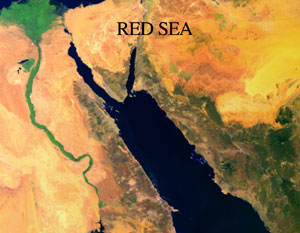
In one sense or another, we are all Living on an Island. The continents are buoyant rock masses that are floating in the Earth’s mantle-asthenosphere and surrounded by water at the surface. Earth’s surface is in constant motion and the ocean basins are continually evolving. The image of the Red Sea on this page is an example of some of the most recent change—an ocean basin is forming! We’re going to spend Lesson 2 exploring the Origin of the Ocean Basins and learning about how Sea Floor Morphology relates to the processes that have shaped the current ocean geometry. As I suspect you know, this all starts with Plate Tectonics and Sea Floor Spreading.
By the end of this lesson you should have a deeper understanding of: plate geometry and kinematics, the role of earthquakes, hot spots and how they relate to volcanic edifices, and continental margins. One of the things to think about this week is how you might develop a teaching module on Plate Tectonics.
What will we learn in Lesson 2?
By the end of Lesson 2, you should be able to:
- Explain the basic tenets of plate tectonics including relative and absolute plate motion.
- Use spherical trigonometry to calculate linear and angular distances on Earth’s surface. Employ this knowledge to work with plate motion vectors
- Use on-line resources to calculate rates of plate tectonic motion.
- Explain hot spots at a basic and sophisticated level, including how they can be used to determine relative plate motion, past theories of their origin, the concept of “Mantle wind,” and current ideas about their origin.
- Describe the Wilson Cycle and related concepts of Sea Floor Spreading.
- Discuss Earth’s internal structure, including the relationship and distinctions between chemical classifications (Crust, Mantle, etc.) and rheologic classifications (Lithosphere, Asthenosphere…).
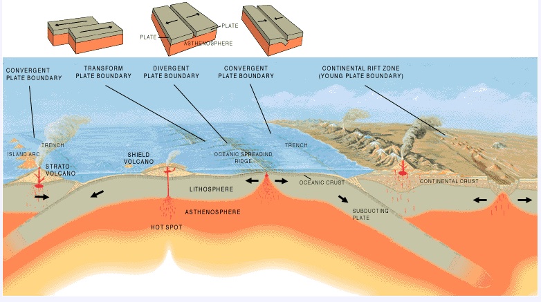
- Readily point out examples of the three basic plate boundaries and their tectonic, seismic and volcanic manifestations at Earth’s surface.
- Use on-line resources to construct maps of the ocean floor
What is due for Lesson 2?
The chart below provides an overview of the requirements for Lesson 2. For assignment details, refer to the lesson page noted. Due dates are listed in this table and in Canvas.
| REQUIREMENT | LOCATION | SUBMITTED FOR GRADING? |
|---|---|---|
| Activity 1: In five easy parts... | see "activity 1" in lesson 2 menu | Yes - You should put a file with your answers in the Canvas dropbox, due June 16th |
| Activity 2: Make map images and comment in a discussion forum. | see "activity 2" in lesson 2 menu | Yes- You should put a file with your answers and comments in the Canvas dropbox |
| Activity 3: Hotspots, background reading and discussion | see "activity 3" in lesson 2 menu | Yes- Discussion responses will be graded. |
Questions?
If you have any questions, please post them to our Questions? discussion forum (not e-mail), located in the Discussions menu in Canvas. I will check that discussion forum daily to respond. While you are there, feel free to post your own responses if you, too, are able to help out a classmate.
Overview
We need a basic understanding of plate tectonics in order to appreciate how the ocean basins have evolved over geologic time and how they will evolve in the future. I suspect that many, if not all of you, are experts on plate tectonics, and the M. Ed. program at Penn State has a course devoted to the Solid Earth (Earth 520), so we won’t cover things in an exhaustive/comprehensive fashion. Instead, we’ll pick a few representative activities that will highlight the connections we need for Oceanography and help you to see what additional background would be useful for you.
A brief background on Plate Tectonics and Continental Drift
The notion that plates move has been around since at least early 1900's. Alfred Wegener, a German Meteorologist, proposed the theory of Continental Drift. He used a variety of observations to argue that the continents had moved and broken apart –including the shapes of coast lines, palaeontological and botanical data, and geological data. But he lacked a credible theory for motion. Physicists of his day dismissed the notion that the continents could move because they thought Earth’s interior was solid and rigid. Nevertheless, various people worked on the theory and proposed modifications. One such was Alex Du Toit, a south American geologist who collected geologic observations from both sides of the south Atlantic and published them in the 1930’s. A number of discoveries in the 1950’s and early 1960’s, including age dating of rocks and magnetic signatures in rocks, led first to the theory of ‘sea floor spreading’ and then to the theory of plate tectonics. A naval captain, Harry Hess, proposed sea floor spreading on the basis of bathymetric profiles he made in the pacific. His data showed that ocean depth increased systematically and symmetrically from a long, axial ridge. Hess’ data were combined with other key observations (including magnetic stripes, heat flow, seismicity along plate boundaries) and ideas (mantle convection) to form the theory of plate tectonics.
Tenets of the theory:
- Plates are rigid
- Earth is a perfect sphere (and points on it can be specified with a radius vector)
- Plates move tangential to the radius vector.
- Material is created and destroyed at spreading ridges and subduction zones, but not at transform boundaries.
- Transform faults form small circles to poles of rotation.
Three important issues for plate tectonics
Issue #1: Earth’s Internal Structure
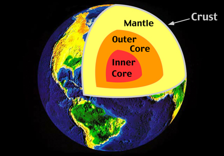
The Earth’s internal structure is made up of three layers called the crust, mantle, and core. The crust is the outermost layers made up of solid rocks mostly silicon and aluminum. The mantle is the layer beneath the crust and made up of mostly silicon and magnesium. The mantle has two layers called the upper mantle and the lower mantle, collectively called the lithosphere. The oceanic and continental plates are in the mantle. The core is the innermost layer of the Earth and is made of solid iron and nickel. The outer core is a liquid layer beneath the mantle and the inner core is the center of the Earth.
Note that there is a distinction between features defined by chemical composition (Crust, Mantle, Core, as shown in the sketch) and those defined by rheology (Lithosphere, Asthenosphere, Mesosphere --not shown here).
Check this out!
A few cool facts:
- The density contrast between the Lithosphere (roughly 2.5 to 3 gm/cc) and the Atmosphere above it (roughly 0) is not nearly as big as that between the Outer Core (roughly 11 gm/cc) and the base of the Mantle (roughly 6 gm/cc).
- Good place to learn more about Earth Structure. [24]
- Better place to learn more about Earth Structure. [25]
- Look at how thin the Crust is! Challenge: Find a better Earth analog than a Major League Baseball (see Activity 1)
Click for text description of the common ellipsoids and spheres image
Text Description of Common Ellipsoids and Spheres Table
Common Ellipsoids and Spheres Ellipsoid/Sphere Radius Thickness/ Radius: Crust Thickness/ Radius: Mantle Thickness/ Radius: Outer Core Thickness/ Radius: Inner Core Earth
Radial Thickness (km)6371†km 0.0055
35 km0.4481
2855 km0.3547
2260 km0.1916
1221 kmMoon 1738 km - - - (?)1 Titleist Golf Ball 21.3 mm 0.1315 0.2253 - 0.6432 Baseball (Major League) 36.3 mm 0.0716 0.4738 0.1680 0.2865 Baseball (Little League) 35.6 mm 0.0702 - - 0.9298 Foam Baseball 30.8† mm -- - - 1 Softball (Worth, Blue Dot) 46.9 mm 0.0490 - - 0.9510 Your_favorite_ellipsoid (?) _______ _______ _______ _______ _______ †Radius of volume equivalent sphere. Earth is an oblate spheroid; it's polar radius is 6357 km and it's equatorial is 6378 km. Foam Baseball's radii across and with the seams are 30.2 and 31.4 mm, respectively.
Issue #2: Plate Boundaries
There are three types of plate boundaries:
- Divergent,
- Convergent, and
- Transform.
In the parlance of structural geology: Divergent Boundaries correspond to normal faults, Convergent Boundaries correspond to thrust (or reverse) faults, and Transform Boundaries correspond to strike slip faults .
Want to learn more?
If you’d like more background on Faulting, see the page on "Faults" [27] from Prof. Eliza Richardson’s course, EARTH 520: Plate Tectonics and People.
Issue #3: Earth is an oblate sphere, which means it is elliptical!
Okay! The main thing is that it's roughly spherical (NOT flat!). The average radius of Earth is 6,371 km and the radius is nearly 22 km larger at the equator than at the poles (it's an ellipsoid, rather than a perfect sphere!). The lithospheric plates move on the outer surface of a sphere, so it's convenient to describe plate motion in terms of a rotation about a point on Earth's surface (or a rotation vector that hypothetically extends from Earth's center to the surface point). This point is called the pole of rotation, or just the rotation pole.
Let's start with a useful formula for the radius:
Earth is not a perfect sphere: its ellipticity can be written:
where Re is the equatorial radius=6378.14 km, and Rp is polar radius=6356.75 km. To first order, the variation in radius with latitude, , can be written:
Want to learn more?
Read about changes in Earth’s shape due to climate events in the following NASA article: "Some changes in Earth's Shape Are Due to Changes in Climate [28]."Map view symbols for plate boundaries
.jpg)
Want to learn more?
Want more background or do you need more help with plate boundaries and plate names? Take a look at This PBS Learning Site [29]
Try this!
Can you identify the type of faulting occurring at each plate boundary in the map below? What type of faulting is depicted between the Nazca and South American plates?
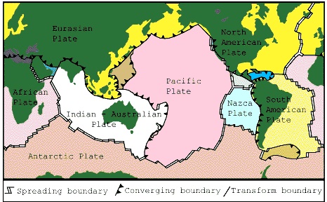
Plate Motion and Activity 1
Let's do something with Plate Tectonics and ask how fast plates move relative to one another? The answer can be found by using plate rotation vectors. Stick with me for a minute or two. This looks more complicated at first blush than it really is. For our purposes, we just need the ability to plug numbers into an equation --so we need to follow the parameter definitions and the equation.
Want to learn more?
See "Simple Euler Poles [32]."
The motion of a point on one tectonic plate relative to another plate can be described by the relative velocity vector v. The velocity v has magnitude and direction and is given by the cross product of the angular velocity vector ω and the plate rotation vector r . The equation looks like this, where the "x" means cross-product. The reason we can't just use distance=rate*time is because we are describing the motion on the surface of a sphere as opposed to making the assumption that it's all flat and distances are simply linear.
v = ω x r
For example, according to one of the accepted models for plate motion (NUVEL 1), the velocity of the North American Plate relative to the Pacific Plate is given by the rotation pole at: 48.7° N 78.2° W and angular velocity 7.8x10⁻⁷ degrees/year (that is: 0.00000078 deg/year.) Therefore, a point on the Pacific plate near Parkfield California, which is at 35.9° N 120.5° W, is moving at 47.6 mm/yr relative to the rest of North America. How long will it take for this point to reach the present location of San Francisco?
How does this calculation work? Download this pdf file for the details [33]. That file contains some useful background. The last page is the example above.
NOTE: Parkfield CA is the site of a National Science Foundation project called EarthScope [34] that has drilled into the San Andreas Fault. See SAFOD Observatory [35] for more details on the drilling project.
One of the first sketches to show tectonic plates
Note the three types of plate boundaries (compare to the figure on the previous page) and the definitions of lithosphere, asthenosphere, and mesosphere. Lithosphere means the rigid part and thus the bottom of it is defined by an isotherm (do you know why?). The base of the lithosphere is typically taken as 1300° C. Note that the plate thickens as it moves away from a divergent spreading center. Mid-ocean ridge systems are hot (they are volcanoes!) and thus ridges are relatively buoyant, which means that they have relatively higher elevation than regions around them. Ocean depth increases systematically with distance away from mid-ocean ridge systems. We'll look at this more closely in Activity 3.
Note in the sketch below that the Earth and its plates are portrayed as a block instead of a sphere. If you think spherical geometry is difficult to work with, you are right. It's hard to visualize in your head and not so easy to sketch, either.
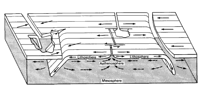
Plate motion vectors
You can always use vector algebra to calculate linear velocity v from the position vector r and the angular velocity vector ω, but there's an easier way to get the magnitude of the velocity by using the solid angle between the pole of rotation and the location of interest (see below). The solid angle can be obtained using spherical trigonometry:
cos a = cos b cos c + sin b sin c cos A
where a is the solid angle of interest, b is the co-latitude of the location on Earth's surface, c is the co-latitude of the plate rotation pole and A is the surface angle between the pole and the location (that is: A is the difference between the longitude of the pole and the longitude of the location).
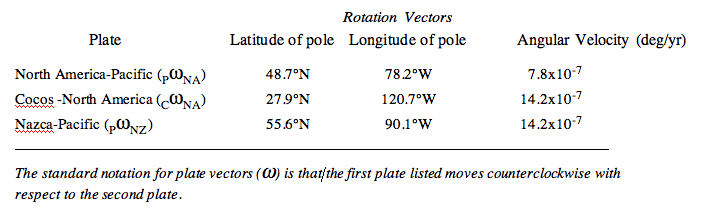
Plate Motion Vectors
Credit:Prissy.US
Click for text description of the plate motion vectors table.
Text Description of Rotation Vectors Table
| Plate | Latitude of pole | Longitude of pole | Angular Velocity (deg/yr) |
|---|---|---|---|
| North America-Pacific (PNA) | 48.7°N | 78.2°W | 7.8x10⁻⁷ |
| Cocos-North America (CNA) | 27.9°N | 120.7°W | 14.2x10⁻⁷ |
| Nazca-Pacific (PNZ) | 55.6°N | 90.1°W | 14.2x10⁻⁷ |
The standard notation for plate vectors () is that/ the first plate listed moves counterclockwise with respect to the second plate.
Some background on Spherical Trigonometry
To work with plate motion vectors, and to calculate the linear velocity of points on Earth's surface, we need to know the distances between various points on the globe. A useful analogy is that of linear and angular velocities associated with Earth's daily rotation. That is, the angular velocity is the same everywhere on Earth. All points rotate through 360° (2 pi radians) in 24 hours. But the linear velocity, on Earth's surface, depends on where you are relative to the rotation axis. If you're at the North Pole, then you cover only a small distance, whereas if you're at the equator, then you cover a distance equal to Earth's full circumference in 24 hours (2 pi R). As Earth rotates each day, the linear velocity of points at the Equator is much larger than points near the poles. The same type of thing happens with plate motions. Points that are close to the pole of rotation move with lower linear velocity than points that are farther from the pole. So, we need to calculate the distance between each point and the pole. These next two figures will help show how this works. Remember, for our purposes, we just need to be able to plug numbers into an equation, so we need to follow the parameter definitions and the equation.
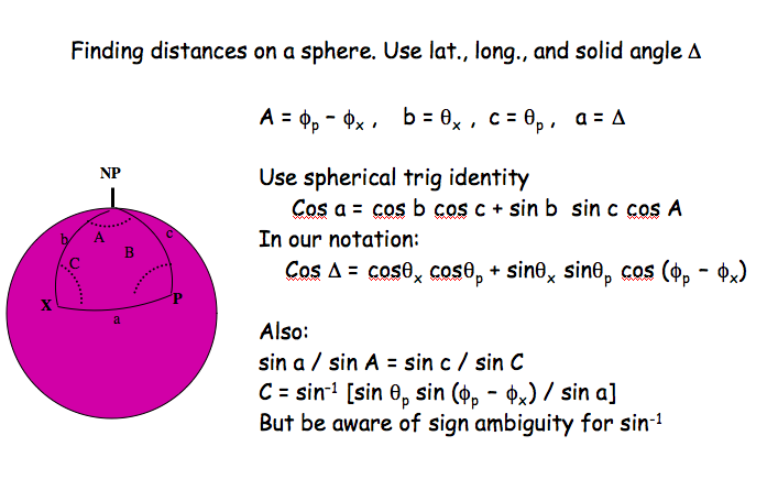
Click for text description of the spherical trigonometry image.
Use spherical trig identity
In our notation:
Also:
But be aware of sign ambiguity for sin-1
In the diagram above, upper case letters refer to surface angles and lower case letters refer to solid angles, measured between lines that extend from the Earth's center to the surface. For a point X at, say, latitude 20° N, the angle b is 70°, because b is measured from the north pole along a line of longitude. In the calculation, it's standard to use the 'co-latitude' b and c. Note that it's easy to get b and c, based on their latitudes. But the same is not true for the solid angle a. That's why we need spherical trig. Surface angles are perhaps more familiar. They are obtained from latitude and are therefore nothing more than a larger-scale version of the angle between the first-base line and the third-base line on a baseball diamond.
Here's an example that will help to fix ideas. Do you follow? If not, please post a question on Canvas.
Click for text description of the spherical trigonometry example image.
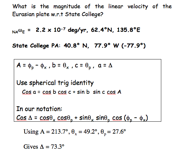
What is the magnitude of the linear velocity of the Eurasian plate w.r.t State College?
State College PA: 40.8°N, 77.9°W (-77.9°)
Use spherical trig identity
In our notation:
Check: Can you verify 73.3 deg. for this example? If not, make sure you're using co-latitude and that your answer is in degrees. Still having trouble? Then have a look at this [36].
Magnitude of linear plate velocity
Once you have the angular distance between the points (Δ), you can get the linear velocity using v = ω R sin Δ. See the last page of this pdf file for a worked example [37].
Activity 1
NOTE: For this assignment, you will need to record your work on a word processing document. Your work is best submitted in Word (.doc), or PDF (.pdf) format so I can open it.
Directions
- Find an analog for Earth's internal structure and measure the relative thicknesses of the layers. Here is an image that goes along with mine (a major league baseball), see details of my numbers on the previous page:
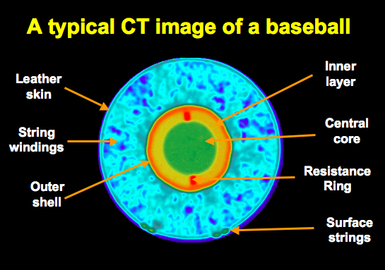 A typical CT image of a baseball
(Are you a fan? Here's a short set of ppt images showing how baseballs have changed over the years.) [38] - Using the formula given on the previous page, calculate Earth's radius at your location. Here's how: look up the latitude of where you are, and then plug-and-chug. This is the relevant equation, so you don't have to go back and find it again: in which Re is the equatorial radius=6378.14 km and lambda is your latitude, and f is the Earth's ellipticity: can be written: where Rp is polar radius=6356.75 km.
- Now, we're ready for a real problem. Calculate the rate of motion between the Pacific Plate and the North American Plate at Hollywood, CA. (I worked the example of the Golden Gate Bridge for you.) I expect that you will show enough of your work so that I can follow how you did the calculation. At the least, you should list all of the parameters and factors used in your calculation. Even better is to paste in your calculation from Google or elsewhere, as in this example: http://www3.geosc.psu.edu/~cjm38/540/sphericaltrigExample.html [36]
- 37.8 N 122.5 W (the golden gate bridge) [39]
- 34.1° N 118.3° W (Hollywood, CA)
- Check both sites using the plate motion calculator [40] at the UNAVCO Web site.
NOTE: To start, you can enter just the latitude and longitude of the point of interest and hit submit. You'll get an answer, with default parameters. Hmm, does it work to just copy/paste in the numbers above? What happens if you write 122.5 W vs. -122.5? Can you include the ° symbols?
For our example problem, you should set the Reference to "PA Pacific" when doing the Golden Gate case, and "North America" when doing Hollywood (what happens if you choose Pacific for the Hollywood case?). You can also try NNR (no net rotation). Play around with this a bit. It's useful!
Under "Model" select "All of the above" so that you can see the range of predictions. Tell me your thoughts on why there are differences in the predicted rates of motions. What happens if you use a different frame of reference?
- Go to the UNAVCO Web site [41] and determine a plate motion rate using their GPS data for the Mission Viejo, CA station. Do two things: calculate a linear velocity like we did in #3, having read the latitude and longitude of this station on its web page. Then use the plots of GPS data to calculate an approximate linear velocity using the Pythagorean theorem, as in north2 + east2 = total2. The link will take you to the UNAVCO page for Mission Viejo, CA (SBCC). (Note: The folks at UNAVCO sometimes modify their web page. If you have trouble finding the data, use this file [42]).
- You have now calculated plate motion at three different places on the North American plate with respect to the Pacific plate using spherical trigonometry. You have compared those calculations to two other methods (using UNAVCO's calculator and using properties of right triangles). Discuss in a few sentences the similarities/differences between the different calculated values and whether you think the differences are due to rounding errors, geographic location, other assumptions, and so forth. If you wanted to make an estimate the quickest way, which method would you use? If you wanted the most accuracy, which would you choose?
- Save your document as either a Microsoft Word or PDF file in the following format:
L2_activity1_AccessAccountID_LastName.doc (or .pdf).
For example, student Elvis Aaron Presley's file would be named "L2_activity1_eap1_presley.pdf"—this naming convention is important, as it will help me make sure I match each submission up with the right student!
Submitting your work
Upload your paper to the "Lesson 2 - Activity 1" dropbox in Canvas by the due date indicated on our Course Schedule.
Grading criteria
See the grading rubric [43] for specifics on how this assignment will be graded.
Activity 2; Motion Under the Ocean, Hot Spots
Activity 2
NOTE: For this assignment, you will need to record your work on a word processing document. Please submitted in Pages, Word (.doc), or PDF (.pdf) format so I can open it. Also, this doesn't have to be long. What I want is the figures I mention and some text to go with them that describes what you did and what you concluded. If we were in a classroom together I imagine this would be like an in-class or in-lab exercise, meaning I'm expecting you could do a reasonable job in an hour or two, depending on your reading speed and any prior experience with Google Earth.
Directions
- First, read this short paper. It's important background for mid-ocean ridges and the bathymetry around them:
- Macdonald, K.C. and P.J. Fox, The mid-ocean ridge [44], Scientific American 262:72-79, 1990.
- Download Google Earth [45] and spend enough time with it to make an image of the ocean floor. In particular, look at the bathymetry around a mid-ocean ridge spreading center. Paste your image into a word processing document as noted above. Note that you should look at parts 3 and 4 before you complete this.
- In your document, comment briefly on how seafloor depth and morphology varies with increasing distance from a mid-ocean ridge spreading center. For example, I'm hoping you'll produce an image in part 1 that will tie-in with the article noted above. (Can you find some of the features they discuss? If you can, describe where they are. If not, or if you aren't sure, think about any differences in our ability to image the sea floor now versus when the paper in part 1 was written.) Think big, don't limit yourself to a few km from the spreading ridge; consider seafloor morphology at the scale of an entire ocean basin, like this example image of the Ocean Basin [46].
- Look at the Crustal Age [47] Poster [47] from NOAA. Download the image, take a screen shot, or use another approach to make a map of the ocean floor showing seafloor age. Add one or two other features to your map, and describe in a few sentences whether you could use a Web site like this in one of your classes. Paste your images into the word processing doc along with your comments.
- Save your document as either a text, Pages, Microsoft Word, or PDF file in the following format:
L2_activity2_AccessAccountID_LastName.doc (or .pdf).
For example, student Elvis Aaron Presley's file would be named "L2_activity2_eap1_presley.doc"—this naming convention is important, as it will help me make sure I match each submission up with the right student!
Submitting your work
Upload your document to the "Lesson 2 - Activity 2" dropbox in Canvas (see Dropboxes folder under the Assignments tab) by the due date indicated on our Course Schedule.
Grading criteria
See the grading rubric [43] for specifics on how this assignment will be graded.
Activity 3: Discussion about recent hot spot research papers
Now that we are experts on Plate Motions, let's think about how Volcanic Island Chains work and how they can help to understand plate tectonics and ocean process.
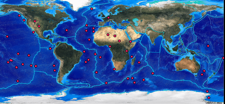
The dots on the map below show locations of major Hotspots on Earth's surface.
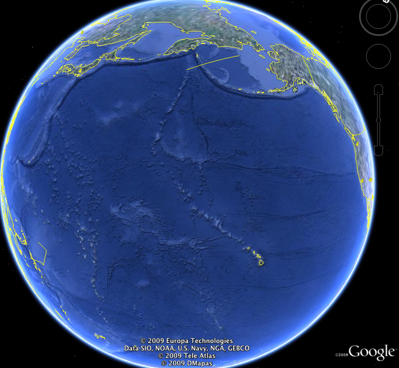
I made the image below with Google Earth. It shows the Hawaiian Island Chain and the Emperor Seamount Chain. Follow the linear track to the northwest from the Hawaiian islands (yellow lines show island coastlines). The features that are not outlined in yellow are below sealevel; they're called seamounts. The Hawaiian chain connects to the Emperor Seamount Chain, which has a more northerly trend. The seamounts are extinct volcanoes. Each one of them was once located over the Hawaiian Hotspot.
Want to learn more?
- More information about hotspots, see "'Hotspots': Mantle thermal plumes. [49]"
Hotspots and Ocean Floor Morphology
Hotspot tracks on the ocean floor were one of the first smoking guns for the theory of plate tectonics, and they were also one of the conundrums. Early evidence showed that hotspots were more or less fixed in space; they did not seem to move relative to one another. This led to the idea that they originated at great depth. But how could a narrow plume of heat, or low viscosity material, rise through the convecting mantle without being offset? Early researchers pointed to the analogy of smoke rising through the atmosphere: on a windy day, the smoke plume was offset, and when the wind changed direction, so did the plume.
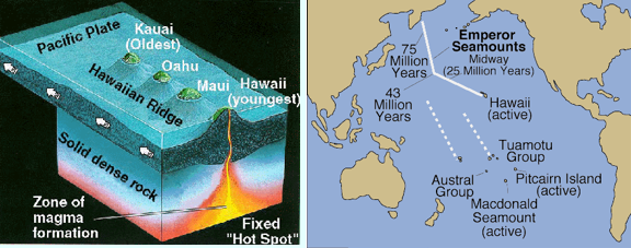
The images below shows a basic idea of how hotspots and linear island chains work.
Activity 3
Directions
- Refer to these short papers:
- Post your responses to the following questions in the discussion area on Canvas for Lesson 2 Activity 3.
- Why do hotspots form distinct volcanic islands, rather than a continuous linear axis?
- What major change occurred recently in our thinking about Hotspots, and what were the data that led people to rethink the way hotspots work?
- Many textbooks say that the change in trend of the Hawaiian Islands and the Emperor Seamounts represented a major shift in the direction of the Pacific plate motion ~ 43 Ma. Is that still thought to be true?
- Read the postings made by other EARTH 540 students.
- Respond to at least two other postings, per question, by asking for clarification, asking a follow-up question, expanding on what has already been said, etc. You should have at least six responses to other postings.
Submitting your work
- I have begun this discussion activity by posting each of the 3 questions to the discussion on Canvas. Please click on the "reply" link that follows each question in order to post your response. To respond to another student's posting, use the "reply" link that follows their posting.
Grading criteria
You will be graded on the quality of your participation. See the grading rubric [43] for specifics on how this assignment will be graded.
Additional Resources
Want to explore these topics more? Here are some resources that might interest you.
Various Web site with links to resources aimed at teachers and students:
- Animations of Plate Motion and Continental Drift, UC Berkeley Site [54]
- Hawaiian center for Volcanology [55]
- University NAVSTAR Consortium is the data warehouse and central facility for GPS and other forms of geodetic data [56]
- Early history of plate tectonics: Discovering transforms and hotspots [57]
Reading the technical/scientific literature:
- Clear As Mud: [58] A concise and stimulating summary of accessibility in scientific literature. Perfect for a discussion of how to write, and how to read, science.
- Summary of Clear As Mud [59] and suggestions for how to read scientific literature. Written by the former director of a Penn State writing center.
Tell us about it!
Have another Web site on this topic that you have found useful? Share it in the Comment area below!
Don't see the "Comment" area below? You need to be logged in to this site first! Do so by using the link at the top of the left-hand menu bar. Once you have logged in, you may need to refresh the page in order to see the comment area below.
Summary & Final Tasks
Reminder - Complete all of the lesson tasks!
You have finished Lesson 2. Double-check the list of requirements on the first page of this lesson ("Lesson 2" in the menu bar) to make sure you have completed all of the activities listed there before beginning the next lesson.
Once you've completed all lesson tasks, make sure you enter the "Teaching and Learning" discussion in Canvas and tell us how you would teach a topic from this lesson in your own classroom
Tell us about it!
If you comments about anything feel free to post your thoughts below. For example, what did you have the most trouble with in this lesson? Was there anything useful here that you'd like to try in your own classroom?
Don't see the "Comment" area below? You need to be logged in to this site first! Do so by using the link at the top of the left-hand menu bar. Once you have logged in, you may need to refresh the page in order to see the comment area below.
Lesson 3
Lesson 3 Introduction
About Lesson 3
In this lesson, we will return to the amazing properties of water and how those properties influence Earth surface processes. We will explore the structure of water molecules and of water itself (yes, water has "structure"), and relate these concepts to important processes, such as the buffering of Earth surface temperature variations and weathering (breakdown) of rocks on land. In addition, we will investigate the composition of sea salt and its origin, as well as some of the exchanges of salt and water between various reservoirs (storage bins) at the Earth's surface. Although based on chemistry (scary or "boring" to some students), this topic has some fascinating elements that can really engage students, including thinking about the importance of salt in human history, debates about the age of the Earth from an ocean perspective, and the potential for extracting metallic riches from the ocean. The topical coverage for Lesson 3 is as follows:
- Ice, water and vapor
- Latent heat, heat capacity, and other unusual properties
- Water as the universal solvent
- Why the sea is bitter
- It’s all about cycles: from vapor to rain to snow to rivers and the ocean (the "Hydrologic Cycle").
- Geochemical residence time
- Salt as a commodity and the age of the oceans
What will we learn in Lesson 3?
By the end of Lesson 3, you should be able to:
- List the important characteristics of ice, water and vapor, and cite why they are important
- Describe latent heat and heat capacity and apply concepts to understanding climate processes
- Explain why water is the universal solvent
- Speak knowledgeably about the origin of salts in seawater
- List the factors that determine seawater salinity and the elemental composition of seawater salt
- Explain the hydrologic cycle and its linkages to water properties
- Explain the concept geochemical residence time in the oceans and what insights it provides.
What is due for Lesson 3?
The table below provides an overview of the requirements for Lesson 3. For details, please see the Course Schedule.
| REQUIREMENT | LOCATION | SUBMITTED FOR GRADING? |
|---|---|---|
| Activity 1: Science Fiction Blog: If Water Behaved Differently | page 8 | Yes - Your discussion participation counts toward your overall class participation grade. This discussion will take place on Canvas. |
| Activity 2: The Residence Time of Salt in the Ocean | page 9 | Yes - Your discussion participation counts toward your overall class participation grade. This discussion will take place on Canvas. |
| Activity 3: End of Unit Quiz (Canvas) | Canvas | Yes. We will activate a set of questions to "test" your understanding of the material a few days before the end of this lesson. The exam should take no more than one hour, but you are welcome to start it and then complete it later. The exam is 'open book.' Feel free to use any resources. |
Questions?
If you have any questions, please post them to our Questions link on Canvas. I will check that discussion forum daily to respond. While you are there, feel free to post your own responses if you, too, are able to help out a classmate.
Ice, Water, & Vapor
Introduction
We will first examine water as a molecule, and then explore the implications of water's molecular structure for its physical behavior and its importance as a "universal solvent." This first section examines the phases of water.
Reading assignment
Read Chapter 6 (pp. 151-182) in Life's Matrix: A Biography of Water by Philip Ball [60], then read the material in this section. Ball, an editor for Nature, has an elegant way of framing the "weirdness" of the water molecule that highlights water's unusual properties. This chapter is a nice treatment to accompany our "drier" outline below.
The Water Molecule
A molecule of water is composed of two atoms of hydrogen and one atom of oxygen. Now, the one and only electron ring around each hydrogen atom has only one electron. The negative charge of the electron is balanced by the positive charge of the one proton in the nucleus. Protons have mass, electrons do not. One electron and one proton: hydrogen has an atomic number of one. In the hydrogen nucleus is also one neutron; no charge but the weight of one proton. One proton, one neutron: hydrogen has an atomic weight of two. The electron ring of hydrogen would like to possess two electrons to create a stable configuration. Oxygen, on the other hand, has an inner electron ring with two electrons, which is cool because that is a stable configuration. The outer ring, on the other hand, has six electrons but it would like to have two more because in the second electron ring, eight electrons make the stable configuration. To balance the negative charge of eight (2+6) electrons, the oxygen nucleus has eight protons. Eight protons and eight electrons: oxygen has an atomic number of eight. The eight protons in the nucleus are matched by eight neutrons. Eight protons, eight neutrons: oxygen has an atomic weight of 16. Hydrogen and oxygen would like to have stable electron configurations but do not as individual atoms. They can get out of this predicament if they agree to share electrons (a sort of an energy "treaty"?). So, oxygen shares one of its outer electrons with each of two hydrogen atoms, and each hydrogen atom shares its one and only electron with oxygen. This is called a covalent bond. Each hydrogen atom thinks it has two electrons, and the oxygen atom thinks that it has eight outer electrons. Everybody's happy, no?
Figure. 1:
O
/ \
H H
However, the two hydrogen atoms are both on the same side of the oxygen atom with an angle of about 105 degrees between them (see Fig. 1) so that the positively charged nuclei of the hydrogen atoms are left slightly exposed, so to speak, leaving that end of the water molecule with a weak positive charge. Meanwhile on the other side of the molecule, the electrons of the oxygen atom give that end of the molecule a weak negative change. For this reason, a water molecule is called a "dipolar" molecule. Water is an example of a polar solvent, capable of dissolving most other compounds. In solution, the weak positively charged side of one water molecule will be attracted to the weak negatively charged side of another water molecule and the two molecules will be held together by a weak "hydrogen bond," and so on. At the temperature range of seawater, the weak hydrogen bonds are constantly being broken and re-formed. This gives water some structure, but allows the molecules to slide over each other easily, making it a liquid.
Water Properties
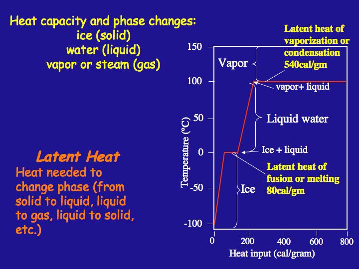
A calorie is the amount of heat it takes to raise the temperature of 1 g of pure water 1 degree C at sea level. Therefore, it would take 100 calories to heat water from 0˚, the freezing point of water, to 100˚ C, the boiling point. However, it would take 540 calories to convert that 1 g of water at 100˚ C to 1 g of water vapor still at 100˚ C. This is called the heat of vaporization. You would have to remove 80 calories from 1 g of water at the freezing point, 0˚ C, to convert it to 1 g of ice at 0˚ C. This is called the heat of fusion.
Water does not give up or take up heat very easily. Therefore, it is said to have a high heat capacity. In Pennsylvania, it is common to have a difference of 20˚ C between day and night temperatures. During the same time frame, the temperature of lake water would hardly change at all.
Water flows easily. It is said to have a low "viscosity." Compare this with motor oil or honey that each have relatively high viscosities (or to the upper mantle that has an even higher viscosity as discussed in class during our "plate tectonics" lectures). If you can't get the honey to flow out of the jar and onto your toast in the morning, you put it in the microwave and "nuke" it, then it flows easily, i.e. increasing the temperature lowers the viscosity. Similarly, warm water is less viscous than cold water.
Pure water has a density of 1.0 g/cm3 at 4˚ C. As you increase or decrease the temperature from 4˚ C, the density decreases. In fact, if you measure the temperature of the deep water in large, temperate-latitude lakes that freeze over in the winter, you will find that the temperature is 4˚ C; that is because fresh water is at its maximum density at that temperature, and as surface waters cool off in the fall and early winter, the lakes overturn and fill up with 4˚ C water. As you add dissolved solids to pure water to increase the salinity, the density increases. The density of average seawater with a salinity of 35 o/oo (35 g/kg) and at 4˚ C is 1.028 g/cm3 As you add salts to seawater, you also change some other properties. Increasing salinity increases the boiling point and decreases the freezing point. Normal seawater freezes at -2˚ C, 2˚ C colder than pure water. Increasing salinity also lowers the temperature of maximum density.
When Water Freezes, It Expands
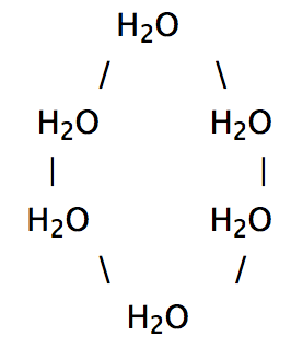
When water is a liquid, the water molecules are packed relatively close together, but can slide past each other and move around freely (that makes it a liquid). When water freezes, however, bonds are formed that lock the molecules in place in a regular (hexagonal) pattern (Fig. 2). For nearly every known chemical compound, the molecules are held closer together (bonded) in the solid state (e.g., in mineral form or ice) than in the liquid state. Water, however, is unique in that it bonds in such a way that the molecules are held farther apart in the solid form (ice) than in the liquid form. Water expands when it freezes making it less dense than the water from which it freezes. In fact, its volume is a little over 9% greater (or density ca. 9% lower) than in the liquid state. For this reason, ice floats on the water (like an ice cube in a glass of water). This latter property is very important for organisms in the oceans and fresh-water lakes. For example, fish in a pond survive the winter because ice forms on top of the pond (it floats) and effectively insulates (does not conduct heat from the pond to the atmosphere as efficiently) the rest of the pond below, preventing it from freezing from top to bottom (or bottom to top). If water did not expand when freezing, then it would be denser than liquid water when it froze; therefore, it would sink and fill lakes or the ocean from bottom to top. Once the oceans filled with ice, life there would be impossible. We are all aware that the expansion of liquid water to ice exerts a tremendous force. If you have ever put a full container of water with a tight-fitting lid, or a can of soda in the freezer, you may have experienced this. Ten cups of water will to turn into 11 cups of ice when it freezes. The force of the crystallization of ice is capable of bursting water pipes and causing cracks in rocks to expand, thus accelerating the erosion of mountains!
The diagram below (Fig. 3) illustrates some changes in the freezing point and the density of pure water, and changes imposed by salt addition. Note that the density of pure water is at a maximum at 4°C, whereas density continues to increase as temperature decreases when the salt content is 35 o/oo (parts per thousand)--near the average salinity of seawater. Also, the freezing point of water is depressed when salt is added (that's why we put salt on icy roads and sidewalks!). We will explore the implications of this later in the course when we consider the circulation of the oceans and the production of "deep" water. Water is only slightly compressible as demonstrated by the small, but measurable, change in density as pressure increases. Pressure is measured here in bars (not the kind you might be savoring about now), where 1 atmosphere (the pressure at sea level) equals = 1.01325 bar = 101.3 kPa. Thus, the maximum pressure of 4000 bars on the graph is equivalent to the pressure at about 4000 meters depth in the ocean (the average depth of the ocean is about 3800 meters). Pressure increases at the rate of one atmosphere every 10 meters (those of you who dive know this). Air-filled volumes, such as human body cavities, cannot withstand the water pressures at depth (this includes most things except for the specially strengthened hulls of submersibles and submarines), but if we could fill our lungs with water and somehow still respire, like fish, we could do some interesting diving. Even at 4000 meters, water has compressed only about 2.3% with respect to the volume it had at the surface (an increase in density of 2.3%, do the calculation given the graphical data below). What was the name of the movie that used that principle? OK, on to the next section...

Salt as a Commodity
We won't dwell too much on salt as a commodity here, but it is an interesting topic for students because salt has played such an important role in human history. There is an excellent book on the subject by Mark Kurlansky titled Salt: A World History. It has extensive information on the uses of salt through the ages, what makes good salt, trade routes, the historical monetary value of salt (Roman soldiers were paid in salt!), the role salt has played in wars, and so on.
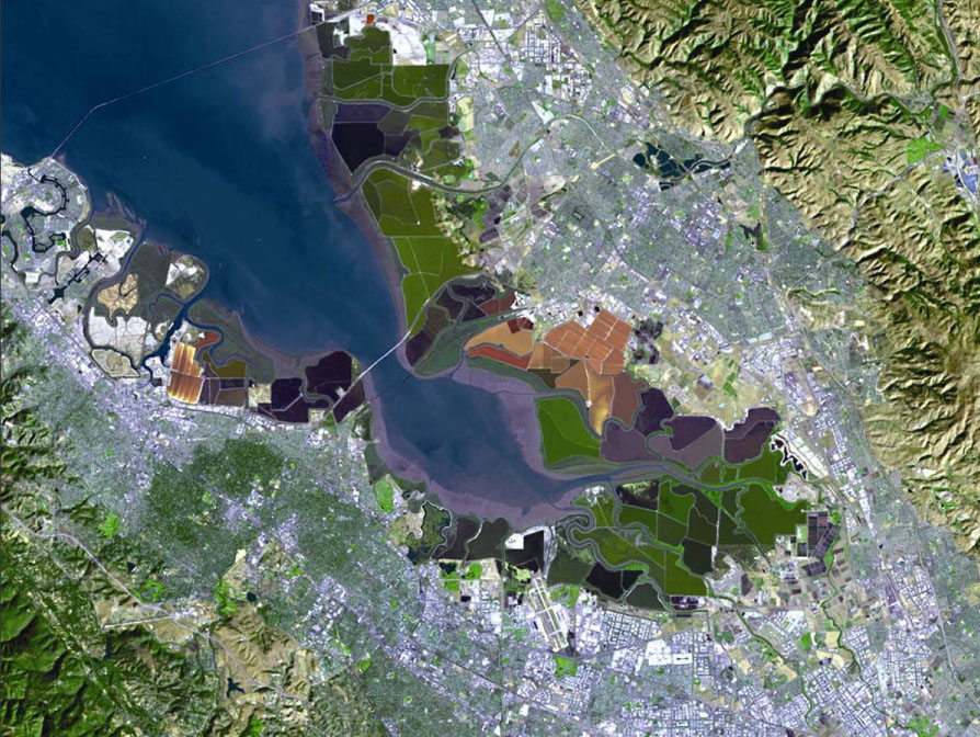
Although salt is mined from strata on land (this salt represents the remnants of ancient oceans that have evaporated and left their salts behind), much is now produced from the evaporation of seawater in carefully monitored salt pans. In the United States, salt mines can be found in New York state (around the Finger Lakes) and New Mexico (near Albuquerque). There is a saltworks (evaporative) in San Francisco Bay (see below). These are the Cargill saltworks near Hayward, California where salt production goes hand-in-hand with wetlands preservation. The reddish ponds are the most highly evaporated--red color is a "bloom" of a salt-tolerant species of photosynthetic dinoflagellates. Most of the active saltworks are in lower latitudes such as Baja, California. The oldest known salt mines are found near Krakow, Poland.
It is intriguing that we can't drink seawater as a means to get our salt (see later section on salt in seawater), but we are totally dependent on this source for the salt our bodies do (and don't) need, whether from ancient oceanic deposits or modern evaporative ponds. There is a good source of information online about salt [62] (follow this link).
Latent Heat & Heat Capacity
These are the relevant physical properties of water and their significance--all of which are shaped by the hydrogen bonding between polar water molecules:
- Heat capacity (highest of all solids and liquids except NH3)
- Latent heat of fusion (highest except NH3)
- Latent heat of evaporation (highest of all substances)
- Thermal expansion (in the first section we showed that the temperature of maximum density decreases with increasing salinity)
- Conduction of heat (highest of all liquids)
- Surface tension (highest of all liquids)
- Dissolving power (the "universal solvent" dissolves more substances in greater quantities than any other liquid)
- Transparency (large absorption of radiant energy)
Heat capacity and latent heat are key properties that allow water (the oceans in particular) to play a major role in "regulating" Earth's climate. Water absorbs solar energy and releases it slowly; thus, larger bodies of water do not change temperature rapidly. Likewise, the high latent heat of vaporization (see below), indicates that when water vapor (derived from evaporation of water at the ocean's surface driven by solar energy receipt at low latitudes) condenses into liquid droplets at high elevations or high latitude, the latent heat is released into the environment. In Lesson 4, we will examine this role in more detail, and we have already alluded to the fact that large lakes can help buffer temperature changes.
Heat Capacity
A direct result of the hydrogen bond in water is the high heat capacity of water. As noted, a calorie is the amount of heat required to raise the temperature of 1 g of water 1 °C. The heat capacity of water compared to that of most other substances is great.
Latent Heats of Melting and Vaporization(refer to figure below)
Closely related to water's unusually high heat capacity are its high latent heat of melting and latent heat of vaporization. A solid converts to a liquid at a temperature called its freezing point and a liquid is changed to a gas at a temperature defined as its boiling point.
When changing the state of any substance, there may be no increase of temperature at that point where a change of state occurs even though heat is continuously being added. All the heat energy is being used to break all of the bonds (e.g. between polar water molecules) required to complete the change of state. The heat that is added to 1 g of a substance at the melting point to break the required bonds to complete the change of state from solid to liquid is the latent heat of melting. The heat applied to effect a change of state at the boiling point is the latent heat of vaporization. The amount of heat required to convert 1 g of ice to 1 g of water, 80 Cal, is termed the latent heat of melting, and it is higher for water than for any other commonly occurring substance. The amount of heat required to convert water to vapor, 540 Cal, is termed the latent heat of vaporization. The figure illustrates energy input to a given mass of water that begins as very cold ice and the temperature path that that mass of water takes with continued heat input. The path from condensation to cooling to ice formation returns energy to the environment.
Surface Tension
Next to mercury, water has the highest surface tension of all commonly occurring liquids. Surface tension is a manifestation of the presence of the hydrogen bond. Those molecules of water that are at the surface are strongly attracted to the molecules of water below them by their hydrogen bonds. If the diameter of the container is decreased, the combination of cohesion, which holds the water molecules together, and the adhesive attraction between the water molecules and the glass container will pull the column of water to great heights. This phenomenon is known as capillarity. This is, in part, what allows plants to stand up--when too much water is lost by evapo-transpiration, they wilt.
Credit:wt.kimiq.com [63]
Heat capacity and phase changes and latent heat.
Heat capacity and phase changes: Ice (solid), water (liquid), vapor or steam (gas)
Latent Heat: heat needed to change phase (from solid to liquid, liquid to gas, liquid to solid, etc)
Ice is from -100 to 0 degrees celsius
Latent heat of fusion or melting 80cal/gm
Ice+liquid at 0 degrees
Liquid water from 0 to 100 degrees
Vapor and liquid at 100
latent heat of vaporization or condensation 540 cal/gm
Water as the Universal Solvent
As indicated in previous sections, the polar water molecule allows water molecules to form bonds with one another. These bonds are referred to as hydrogen bonds. If we consider sodium chloride (salt), a compound containing ionic bonds, we could demonstrate that simply by placing table salt in water, for example, we can reduce the electrostatic attraction between the sodium and chloride ions by 80 times. As more and more ions of sodium and chlorine are freed by the weakening of the electrostatic attraction that is holding them together, they become surrounded by the polar molecules of water--what is termed "hydration."

Water dissolves more substances than any other common liquid by breaking "salts" into component "ions" (e.g. NaCl into Na+ and Cl-) and hydrating those ions to keep them from interacting. Thus, polar water molecules have an attraction for ions (atoms or groups of atoms with a charge), where "cations" are ions with positive charge and "anions" have negative charge. Most elements have high solubilities in water, which means that large concentrations of those elements can build up before the capacity for water molecules to isolate the ions is exceeded. The point at which Na and Cl, for example, would begin to precipitate a salt in seawater is termed "saturation." For NaCl (the mineral "halite") this only occurs from present-day seawater when evaporation occurs and the volume of seawater is reduced to about 10% of its original volume.
Seawater is essentially an NaCl solution which averages a concentration of 35 g NaCl/kg water (or 3.5% salt). Na and Cl compose over 85% of the total dissolved solids (salt), but there are other important ions present. The relative abundance of ions in seawater ranks in order: Cl, Na, SO4, Mg, Ca, K. Together, these ions make up >99% of the dissolved solids in seawater. With only four other elements--HCO3 (bicarbonate), Br, Sr, B, F--we have 99.99% of all dissolved solids. Charges must balance, so the positive charge associated with Na+, Mg+2, Ca+2, K+ equals the negative charge associated with Cl-, SO4-2 (and HCO3-). We don't think you would want it any other way. Think about what the flow of the current would be from the sea to you, sitting on the beach, if the charges were not balanced--shocking!
Salinity varies over a range of about 32 to 37 o/oo in the open ocean as Figure 2 (below) illustrates. Note that areas of highest salinity occur in regions of highest net evaporation, as one might expect.
All other dissolved substances in seawater are at very low concentrations (part per million or billion) (ppm or ppb; 10-6 to 10-9). This Includes important nutrients such as phosphate and nitrate that are cycled by organisms (elements called "bio-limiting") and essential for life. Many metals have trace concentrations (wanna' get rich? There are about 9 million tons of gold dissolved in seawater, which is about equal to all the gold mined on earth throughout history).
As previously indicated, evaporation of seawater produces a predictable sequence of mineral salts (minerals become saturated at a certain point). After evaporation of a few % of water mass CaCO3 (calcite) precipitates; after evaporation of 81%, CaSO4 (gypsum) is fully precipitated; after evaporation of about 90.5%, NaCl (halite) is fully precipitated; at 96% evaporation, the K and Mg salts (w/ SO4 and Cl) drop out. There is enough salt in the ocean to cover land with a layer 170 m thick. Natural deposits from ancient oceans like this are called "evaporites."
Why the Sea is Bitter
The primeval ocean... must have been only faintly salt. But the falling rains
were the symbol of the dissolution of the continents. From the moment the
rains began to fall, the land began to be worn away and carried to the sea. It is
an endless, inexorable process that has never stopped--the dissolving of the
rocks, the leaching out of their contained minerals, the carrying of the rock
fragments and dissolved minerals to the ocean. And over the eons of time,
the sea has grown ever more bitter with the salt of the continents.
--Rachel Carson, The Sea Around Us
Rachel Carson provided this poetic statement about the evolution of seawater chemistry over time in her book, first written in 1950. It is an interesting statement about the prevailing thought of the time--that ocean salinity evolved slowly and progressively and that rivers were the only source of salt. Both of these ideas are incorrect in light of more recent scientific investigations. We will highlight these issues in this section of Lesson 3 as they lead us to some interesting concepts and calculations. In defense of Rachel Carson, a native Pennsylvanian and the forebearer to the modern environmental movement, her failure to correctly describe the system is a function of the huge scientific advances that have been made in the geosciences, beginning in the early 1960s. The concept of plate tectonics was in its nascency in the 1950s and was not widely accepted by the geoscience community until definitive evidence in support of it in the 1970s. Rachel Carson had no idea that the mid-ocean ridge hydrothermal system existed because no one observed a submarine hot spring until 1977 (Galapagos at 2500 meters depth). We can forgive her her ignorance, right?
As the Earth cooled over 4 billion years ago and water began to condense in the oceans (it probably originally condensed and fell as rain), that first water probably did not have a very high salt content. This water was outgassed along with other volatiles from the Earth's interior (mantle) and possibly also accumulated from cometary impacts. Some geologic evidence suggests that the bulk of the oceans were already formed by about 3.8 billion years ago(Ga). But very quickly various chemical ions must have dissolved in water as it bathed or passed over freshly formed igneous rocks (probably mostly basaltic in composition initially), and began to be washed into the pools that eventually grew into the oceans. Water is a remarkable substance (see write up on the "Physical Properties of Water”). The "polar" water molecule allows it to interact with and isolate charged chemical ions (elements with unfilled electron shells that are dissolved in the water), such as Na+ and Cl- in solution. These chemical ions, when dissolved in water, are commonly called "salts." It perhaps took hundreds of millions of years for the ocean to accumulate significant amounts of these salts as the result of the operation of the global hydrologic cycle. In a nutshell: ever since atmospheric water vapor could condense into rain, water has fallen onto the land surface and drained eventually, through rivers and groundwater, into the oceans. The water that falls on the land dissolves minute amounts of salt (called "rock weathering") during its passage over the land. It carries that salt to the ocean. In the meantime, heat from the sun provides the energy to cause more evaporation. The evaporated water then condenses and falls again as rain on land (essentially replacing water that flowed into the sea), and thus continues the cycle. Seawater salts essentially cannot evaporate and, therefore, when the ocean water evaporates, salt remains behind.
The ocean, of course, is constantly losing pure fresh water through evaporation and receiving small amounts of dissolved salt from the river and groundwater coming in. While it would seem that the oceans should be getting saltier over time, the record of sedimentary deposits, called "evaporites” (see the experiment below, also discussed in class), from ancient oceans and the continuity of life as evidenced in the fossil record, indicate that this does not occur. Interestingly, the salinity of seawater appears to have remained relatively constant (but we will see about this!) at about 3.5 % (35 ppt by weight or 35 grams of salt dissolved in 965 grams of fresh water), at least over the past 500 million years or so, but possibly even since sometime earlier (e.g., probably since about 2 billion years ago or more), after formation of the oceans. Thus various chemical, biological, and tectonic processes must act to remove salts from seawater in the amounts necessary to keep the ocean salt content from varying much.
What Determines the Composition of Seawater Salt?
Although much of the ocean's salt has ultimately come from the weathering of continental rocks, there are other important sources and chemical exchanges between seawater and the Earth. The chemical composition of river water and salty inland lakes is, surprisingly, not very similar to that of the oceans. Average river water contains mostly calcium and bicarbonate ions, while seawater consists largely of sodium and chloride; in fact, only five chemical elements make up more than 99% of salt dissolved in seawater. Why does the chemistry of seawater differ from that of the runoff from the continents? This difference must reflect the other sources of "salt" to the oceans, as well as the dominant processes that remove certain salts by "precipitation." (We will explore this for various elements in Lesson 3, Activity 2).
For example, the upper-mantle layer of the Earth contains huge reserves of the elements found in seawater. Deep sea vents, rift vents, and volcanoes, which expel heat and fluids from the Earth's interior, supply large amounts of certain salts through outgassing. In the case of Na (sodium) and Cl (chloride), rock-weathering supplies most of the sodium ions, whereas outgassing of volatiles supplies chlorine. Na and Cl are so strongly enriched in seawater though because they are not used by organisms and do not precipitate out very easily except under highly evaporative conditions in salt ponds or isolated basins where they precipitate as evaporite minerals. These kinds of salts are said to have long "residence times" in seawater compared to other elements (e.g. nutrients such as nitrogen and phosphorus, silica, bicarbonate, and certain others are cycled very rapidly). Interaction (chemical exchange) of seawater and hot basalts at mid-ocean ridges (remember the "hydrothermal circulation" discussed in Lesson 2?) supplies a significant amount of Ca (calcium) to the ocean, while leaving behind an equivalent amount of seawater Mg (magnesium) in the resulting altered basalts. This process constantly modifies the amounts of Ca and Mg in seawater. In addition, seawater contains a lower relative proportion of dissolved silica (SiO2), Ca, and bicarbonate (HCO3-) than river water does. This is because certain groups of marine plants and animals remove these components very rapidly to form their hard parts (skeletal material such as shells or "tests").
Keep in mind that during evaporation or dilution by fresh water, the salt content (salinity) increases or decreases respectively. However, the ratio of each salt component in seawater to another (e.g Na/Cl or Ca/Mg) remains constant as long as the salinity does not increase to the extent that mineral precipitation begins. This is called the “Principle of Constant Proportion” and is useful for understanding external inputs or outputs of various elements that might change the ratio of one element to another.
An Experiment:
Here is a simple experiment that illustrates the process of evaporation and precipitation of salt from seawater that might reinforce this concept for students (we commonly see college students who don’t think about evaporation leaving the salt behind as a mechanism for increasing saltiness). This experiment will only work in a reasonable time during a warm, dry period (in your “not so fair” state of Pennsylvania, these are few and far between). You should use any sort of clear glass jar and fill it to some line that you have marked on the side of the vessel. First, fill the jar with pure (distilled, not tap) water to the line. When the water evaporates completely (look for any residue), there should not be any. Now mix a mild salt-water solution (use common table salt to 3.5 g in about 100 ml of pure water) or use seawater if available, and again fill the jar to the line with the solution. When that evaporates, again look for residue (if you could scrape it all out and weigh it, the weight of salts left behind as precipitates should be 3.5 g). Of course, the water evaporates into the air and the salt remains behind. If seawater (even artificial aquarium sea salt) is used, one might even observe salts of different minerals precipitating out as the water level in the glass drops. Minerals of different salt components have different saturation points (lower solubility), such that calcite (calcium carbonate, CaCO3) precipitates first, followed by gypsum (CaSO4), halite (NaCl), sylvite (KCl), and finally some small amounts of various magnesium sulfate salts, etc.
It's All About Cycles
Yes, water cycles (the hydrologic cycle) and geochemical cycles (tracing the paths of various elements to and from seawater). Figure 1 is a conceptualization of the hydrologic cycle (source, USGS). As you are undoubtedly aware, solar energy drives the cycle of evaporation of water from the ocean surface (leaving salt behind), raining out on the continents, and returning to the ocean in rivers (surface runoff). This water does do work on the land surface. Eroding solids and dissolving minerals. Eventually, much of the dissolved material becomes seawater salt. In a geochemical cycle, plate tectonics causes uplift and exposure of "fresh" rocks, which can be weathered by water (and carbon dioxide). Carbon dioxide is driven out of the Earth's interior during volcanism. This is part of the cycle. So, if rock weathering is such an important process, does ocean chemistry simply reflect the chemistry of rivers, only more concentrated? Can the chemistry of the oceans be related to the inputs of rivers alone? We've already examined why water is a powerful solvent, now let's look at the whole picture. The ocean is not simply concentrated river water.
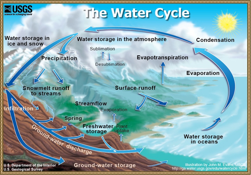
Have you heard Bill Nye's rap version of the Hydrologic cycle? "Water Cycle Jump" Here's a link, but if it doesn't work, please search youtube and find it: Bill Nye the Science Guy - Water Cycle Jump [65].
In fact, the ocean has a much different chemical composition from average river water because, like water, salts are cycled as well. Some salts build up in seawater over time, while other elements are rapidly used, stripped from seawater into organic matter and skeletons of marine organisms or extraction through alteration of near-seafloor basalt in the midocean ridge hydrothermal system.
Rivers supply a large proportion of dissolved solids to the oceans, but river chemistry is very different from seawater.
In rivers the abundance of elements is HCO3, Ca, SO4, SiO2 (1st 4= 80%), then Cl, Na, Mg, K. Rivers are essentially >35% dissolved inorganic carbon (HCO3 or CO3). Compare this with ocean chemistry in the previous section. The difference in chemical compositions between rivers and ocean reflects sedimentation (precipitation) processes and other inputs/exchanges, such as basalt-seawater reactions at midocean ridges. Activity 2 will help you develop an appreciation of geochemical cycling.
We can examine the "reactivity" of an element in the oceans by looking a the "residence time" of that element--on to the last section...
Geochemical Residence Time
Need a break? Listen to this from Tom Lehrer--it'll brighten your day... [66]
Every one of these elements is present at some concentration in seawater. As you have seen, some elements have high concentrations (e.g. Na, Cl) whereas others (e.g. Au or Fe, etc.) have very low concentrations. Very few elements are near saturation (the maximum amount that could be held in seawater of a certain salinity, temperature, and pressure). The chemistry and behavior of elements differ among the various groups (for example redox-sensitive metals vs. alkaline earths).
Residence time is the average time that a substance remains in solution in seawater. It can be calculated for any element by a standard equation. Note that this is cast in terms of the riverine input only (Activity 2 will ask you why this could be incorrect):
Residence Time (yrs.) = Total amount ion in seawater (kg) / Input rate (kg/yr)
where Input rate = Avg. ion conc. in rivers (kg/km3) x River discharge (km3/yr)
Let's consider an example: Here's one for the residence time of water in the ocean. Click here for the ppt file [67] and here for the pdf file. [68]
What is the residence time of all of the salt in seawater? This is an interesting consideration because, in the past, this question was used to argue something about the age of the Earth (How long would it take rivers to deliver all the salt in seawater today?). There are about 5 x 10²² g of dissolved solids in oceans, and rivers bring in about 2.5 x 10¹⁵ g of dissolved solids per year. Think about it. It should only take about 2 x 10⁷ years (20 million years) to bring the oceans to their present salinity, but we know that the oceans are 3.8 billion years old, and if rivers have been providing approximately the same input through time, and if the oceans have maintained approximately the same composition through time, there has to be an output of material that balances the inputs; otherwise, we are wrong about the age of the Earth and its oceans, and that, for various reasons, seems unlikely. This question is still worth exploring with your students because it gets them to think about the dynamic Earth. Interestingly, scientist John Joly (Irish), first tried this calculation around 1901 and obtained an age for the Earth of 90-100 million years. This was too long to suit Irish Archbishop Usher's (1654) supporters who, based on biblical genealogy, believed that the Earth was created in 4004 BC.
You will calculate the residence time for several elements to gain insights into their rate of cycling through the ocean system. Think about what it means to have a long residence time vs. a short residence time. For example, we like to think of Penn State as a system. Students come in; students go out. If we simply assume that all students graduate and that the total number of students allowed at the University Park campus does not change, we can calculate the average residence time of a student at the main campus. There are about 42 thousand undergraduate students, with just over 8 thousand students admitted per year. Residence time? Just over 5 years (ouch!). Of course, we have glossed over the details, right? How many students simply left without their diplomas? You get it--it's the same for geochemical cycle considerations of residence times. We tend to simplify, thereby missing some of the important stories.
A cycle of elements moving in and out of the Earth's lithosphere, biosphere, hydrosphere, and atmosphere. Elements ( rocks) get weathered and is transported in solution or suspension to the ocean(hydrosphere). Sediments formed in the ocean may be compacted to join the geologic cycle, becoming sedimentary, metamorphic, and perhaps ultimately new igneous rock.
Seawater Properties Activity
Activity: Is the Chemical Composition of Seawater Constant? Do All Elements Behave Alike?
For this activity we will investigate the behavior of some of the elements in seawater in order to understand their sources, sinks, and cycles through the ocean, and to help us decide whether ocean chemistry has been constant through time. For this purpose we will have you research two different chemical elements (partly of your choosing) to obtain the necessary information.
Directions
- Choose one element from each of two groups, for a total of two elements (I'm hoping that we don't have overlap, so please tell us what you've chosen)
- Group 1: Na, Cl, K, Mg, S
- Group 2: P, Ca, Si, N, Ba
- To start, go to MBARI [69] for information about chemical elements in seawater. You will find a periodic table (you may need to do a search in the upper right corner), "residence times," and other information on most of the elements.
- Find and list the following information for each element you chose from Groups 1 and 2:
- concentration in seawater (use g/kg)
- total mass in seawater (in metric tonnes or kg)
- amount that could be held in seawater at saturation (and percent saturation)
- known sources of the element to seawater (e.g. rivers, hydrothermal, meteoritic or cosmic, etc.)
- known sinks (extraction from seawater through hydrothermal alteration of seafloor, sedimentation, etc.)
- cycling (is the element bio-limiting, bio-intermediate, or bio-inert?)
- Do the following calculations and answer the following questions:
- Calculate the oceanic residence time for each of the two elements you have chosen to investigate.
- How does the Group 1 element you chose differ from the Group 2 element? Why are they different?
- Why might the inferences you draw from the "residence time" calculations be in error?
- Post your answers in the discussion board on Canvas: Lesson 3, Activity 2: The Residence Time of Salt in the Ocean.
- Read the postings made by other EARTH 540 students.
- Respond to several posts by asking a follow-up question or by asking for clarification and/or expanding on their theme.
Submitting your work
- Begin by posting. To respond to another student's posting, use the "reply" link that follows their posting.
Grading criteria
See the grading rubric [12] for specifics on how this assignment will be graded.
You are now ready for the End of Unit Quiz, which will open on Canvas on the dates given in the Course Schedule
Additional Resources
Various Web sites with links to resources aimed at teachers and students:
- NASA SeaWifs Ocean Color Page--Satellite-generated Maps of Ocean Productivity [70]
- eWOCE Ocean Sections for various parameters (mostly chemical) [71]
- Global Maps of Climatological Data (e.g. Sea-surface Temperature)
- Chemical Elements in Seawater--MBARI [72]
A great (huge) book written about the importance of Salt in human history:
- Kurlansky, Mark (2003) Salt: A World History. New York: Penguin Books.
Tell us about it!
Have another Web site or printed piece on this topic that you have found useful? Share it in our Comment space below!
Summary & Final Tasks
Reminder - Complete all of the lesson tasks!
You have finished Lesson 3. Double-check the list of requirements on the first page of this lesson (Lesson 3 in the menu bar) to make sure you have completed all of the activities listed there before beginning the next lesson.
Once you've completed all lesson tasks, make sure you enter the "Teaching and Learning" discussion in Canvas and tell us how you would teach a topic from this lesson in your own classroom
Tell us about it!
If you have anything you'd like to comment on, or add to, the lesson materials, feel free to post your thoughts below. For example, what did you have the most trouble with in this lesson? Was there anything useful here that you'd like to try in your own classroom?
Don't see the Post new comment area below? You need to be logged in to this site first! Do so by using the link at the top of the left-hand menu bar. Once you have logged in, you may need to refresh the page in order to see the comment area.
Lesson 4
Lesson 4 Introduction
The Global Thermostat. The Ocean-Atmosphere-Climate Connection
About Lesson 4
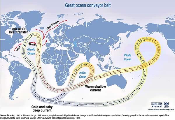
In this lesson, we have the ambitious task of tackling the heat distribution on Earth and it's role in dictating ocean circulation, atmospheric circulation, and Earth's climate.
By the end of this lesson you should have a deeper understanding of the role of the oceans and atmosphere in heat transfer on Earth, the structure of the oceans including surface water and deep water, thermo-haline circulation including patterns and the factors that drive flow, the Coriolis effect and Ekman transport, large-scale atmospheric circulation, oceanic gyres, and boundary currents in the ocean basins.
This figure incorporates many of the topics we will cover in Lesson 4. Note the Gulf stream in the North Atlantic and the sea-to-air heat transfer associated with it. Also note the three dimensional nature of ocean current flow (the conveyor), which includes warm surface currents and deep currents.
What will we learn in Lesson 4?
By the end of Lesson 4, you should be able to:
- Describe the solar energy budget for Earth including variations with latitude of energy input and output.
- Explain how heat is transferred from low to high latitudes by the oceans and the atmosphere.
- Explain the roles of latent heat and sensible heat in energy transfer by ocean currents.
- Describe the pattern of global winds and its relationship to heat transfer.
- Describe the primary structure of ocean waters as a function of depth, including the changes in average temperature and salinity.
- Explain the main factors that determine surface and deep ocean currents.
- Explain the Coriolis effect, it's origin, and it's influence on global winds and ocean currents
- Describe how the Coriolis effect and Ekman transport influence ocean surface currents
- Describe the 'ocean conveyor' and it's role in global heat transfer and climate regulation
- Use on-line resources to construct maps of ocean temperature and salinity
What is due for Lesson 4?
The chart below provides an overview of the requirements for Lesson 4. For assignment details, refer to the lesson page noted. See the Course Schedule (located in the Resources menu) for assignment due dates.
| REQUIREMENT | LOCATION | SUBMITTED FOR GRADING? |
|---|---|---|
| Activity 1: Pressure Belts | page 1 | Yes |
| Activity 2: Ocean Currents and Density | page 4 | Yes |
| Activity 3: Gyres and Surface Currents | page 5 | Yes |
Questions?
Post them to our Questions? discussion forum on Canvas or get in touch by email.
Overview, Solar Energy, Pressure, & Wind Belts
The connections between atmospheric circulation, ocean currents and Earth's climate are both simple and wonderfully complex. We could easily spend the whole semester studying these topics and developing the background for ocean circulation, but we won't. Instead, we'll hit the high points and build a background for understanding ocean currents and thermo-haline circulation. It makes sense to start with atmospheric circulation because ocean surface currents are driven by wind. The basic pattern of surface ocean circulation, including the large-scale gyres, is caused by wind and the factors that produce large-scale wind patterns. We need to start by seeing how solar energy input on Earth and poleward transport of heat by winds sets up large-scale atmospheric cells that produce Easterly and Westerly winds in three main bands from the equator to the poles. The Coriolis effect, produced by Earth's rotation and conservation of momentum, plays an important role here. Ocean structure also plays an important role and we need to look at density driven circulation in the ocean as produced by temperature and salinity: so-called thermohaline circulation. Ocean circulation is three-dimensional and both surface currents and deep water currents play an important role in heat transport. Large-scale ocean currents are impacted by the Coriolis effect, and depth-variations in coupling between surface flow and wind stress produce another important effect, known as Ekman transport, which we will discuss. Ultimately, when we put all the pieces together, the goal is to arrive at a coherent picture of how solar energy, winds, and ocean circulation combine to produce a global thermostat for Earth.
It's all about Blowing Hot Air
This image shows large-scale atmospheric circulation on Earth. Note the three-dimensionality of the circulation. On the right-hand side of the image the arrows show vertical and horizontal air flow as part of six convection cells, three in each of the Northern and Southern hemispheres. The central part of the image shows surface winds blowing from the east (the Trade winds) or the west (The Westerlies) --note that the Polar Easterlies are not easily seen in this image.

Hadley circulation
One of the most important things to understand from this image is that everything is driven by unequal solar heating as a function of latitude. The energy from our Sun is focused on the equatorial region and spread comparatively thinly over the polar regions. This is true on an average annual basis, Earth receives more solar energy at the equator than at the poles. As a result, the land, water, and air, over the equator are warm, and air rises over the equator. This warm air rises through the atmosphere and flows poleward as an upper atmosphere wind that is, essentially, an air-mail package of heat known as a Hadley Cell. The image here has arrows showing circulation in a vertical plane along a line of longitude (just to the east of the African continent) but, of course, this circulation occurs at all longitudes. Hadley circulation is 3D; heat moves poleward in upper atmosphere winds and there is a return flow from north to south (in the Northern hemisphere) that sets up the Northeasterly Trade winds (with the help of the Coriolis effect, as we'll see below).
Pressure belts
The Hadley Cell is set up by rising air over the equator. It begins with warming of air surrounding the equator, which creates a large region of lower surface pressures (due in part to the fact that columns of warm air weigh less than columns of cold air). This belt of equatorial low pressure causes air to be drawn together in a region called the Intertropical Convergence Zone (ITCZ). The convergence of warm, moist air over the equator transports large volumes of air aloft, to the top of the troposphere. This air is confined vertically by the base of the stratosphere and thus spreads out north and south toward the poles.
Because of Earth's spherical shape, the poleward-flowing air is compressed into an increasingly smaller volume as it moves away from the equatorial region. The airmasses also cool as they move poleward. The buildup of cool air aloft causes surface pressures to rise because surface pressure depends on the weight of the entire atmospheric column. The mass convergence and cooling also cause air mass densification, which forces some of the air aloft to sink. At some point, normally ~ 30 deg. North/South, the increase in surface pressures reaches a maximum, marking a belt of subtropical high pressure. Sinking air is dry and characterized by a lack of clouds and precipitation. These regions of subtropical high pressure systems are known for their tranquil weather. Air masses flowing equatorward from these high pressure belts form the Trade Winds that feed the ITCZ, thus completing the Hadley Cell circulation. Similar thinking explains the existence and wind circulation in the Ferrel Cell (labeled the 'mid-latitude' cell in this image) and the Polar Cell.
Activity 1: Pressure Belts
Let's think about the global pattern of atmospheric pressure. Hadley circulation implies a systematic pattern of pressure variation as a function of latitute. One question we could ask involves differences in air masses within a Hadley cell. Referring to the figure above: how do air masses differ between the ascending limbs of a Hadley Cell, over the equator, compared to the descending limb at 30 deg. North?
- Atmospheric Pressure [73] Start by skimming this page. Look at Figures 7d-1 and 7d-4 and read the associated text. (Note: The animation for 7d-4 may open in a separate Quicktime window or be downloaded to your desktop)
- Using these data, let's calculate the average density for air at 30 deg. North compared to that at the equator. You can assume that the atmosphere extends to the 70 km, which is within the Mesosphere. A useful formula for the relationship between pressure, p, density, ρ, gravity, g, and height, h, is: p = ρ g h
- Let's assume that the average air pressure over the equator at Earth's surface is roughly 101.3 kPa (recall: 1 Pa = 1 Newton per square-meter). Does this jive with what you see in figure 7d-4? In this case, what is the average density of air if the column is 70 km tall?
- Now calculate the density at 30 deg. north, assuming an average surface pressure of 102.5 kPa.
- Comment on how air pressure varies as a function of time throughout the year (hint, look at the animation on the web page that you just read).
- Thinking back to what you know about heat capacity and latent heat, do these differences in density make sense relative to your expectations for heat transfer by large-scale winds? Is the air at 30 deg. north likely to be colder/warmer/denser compared to that at the equator?
Submitting your work
Save your document as either a Microsoft Word or PDF file in the following format:
L4_Activity1_AccessAccountID_LastName.doc (or .pages or .pdf)
For example, student Elvis Aaron Presley's file would be named "L4_Activity1_eap1_presley.doc".
Put the file in the DropBox under Lesson 4 on Canvas.
Grading Criteria
See the grading rubric [12] for specifics on how this assignment will be graded.
Redistributing Earth's Heat, Wind, & Currents
Heat redistribution
Earth's heat budget exhibits important variations with latitude. Heat input via solar radiation varies systematically with sun angle, and thus when averaged over a year, we find a simple relationship between latitude and heat absorbed, with more heat received in the equitorial region than in polar regions. The figure below shows this variation along with average annual radiation output from Earth. The dashed lines show the points at which input (heat absorbed at Earth's surface) is equal to output (heat lost via long-wavelength radiation).
Here's a useful animation for thinking about sun-angle variations throughout the year [74].
Now have a look at the figure below. This figure has important implications for wind generation and ocean currents because both are driven by temperature differences, and by heat input between the equatorial and polar regions. Winds and ocean currents play a major role in moving the surplus heat from the equatorial regions to the polar regions. Without this heat transfer, the polar regions of Earth would get colder every year and regions between ~ 35 N and 35 S would get warmer every year. Energy transfer occurs via sensible heat and via latent heat. As you'll recall from Lesson 3, latent heat of evaporation for water is very large compared to heat capacity, so it is no surprise that latent heat is the dominant process, with sensible heat transfer accounting for only a few percent of the heat flux, from ocean to atmosphere, associated with latent heat.
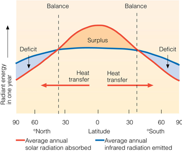
Wind and ocean currents
Winds and ocean currents play a big role in redistributing heat.
This figure shows sea surface wind speed, as derived from a NASA's satellite (Aqua) for the month of November, 2004. The large-scale pattern of surface ocean currents is set up by winds. Note the variations with latitude. Look back at the Hadley circulation and think about the location of the easterlies/westerlies compared to what you see here.
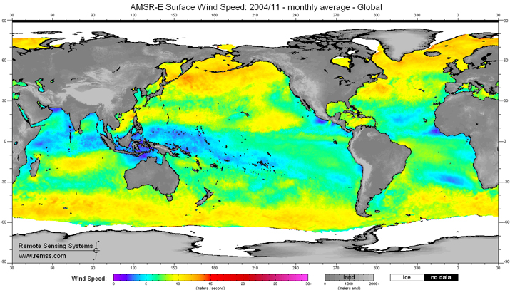
Reading assignment
Read the link below.
- The Atlantic heat conveyor slows [77] Are we heading toward The Day After Tomorrow?
Coriolis and Ekman Transport
For large scale winds and ocean currents, the Coriolis effect is an important consideration because it changes the net direction of heat transport.
Coriolis Effect The Coriolis effect is due to an inertial force that is important in a rotating frame of reference. As you know from Newton's laws of motion, bodies in motion stay in motion unless acted upon by external forces. So, a wind blowing from north to south should go in a straight line, and in fact, it does. The problem is that this straight line does not look straight when referenced to a spinning Earth. There are many on-line resources for the Coriolis effect, so I won't try to duplicate visualizations here, but there are a few things to get straight before looking at a few of them.
- The Coriolis force is given by the Coriolis acceleration times the mass of the object in motion. This is the familiar F = m a.
- The Coriolis acceleration is proportional to the cross product between the (linear) velocity of the moving object and the angular velocity of the rotating frame of reference. On Earth, the angular velocity is given by 360 deg/24 Hr. or 2 π (radians) per 24 Hrs, which is equal to 1.454e-4 radians per sec. The formula is: ac = - 2ω x v
- As you recall from plate tectonics and spherical trigonometry, the magnitude of a cross product like this can be obtained from the magnitude of each vector ( ω and v ) times the sin of the angle between them.
Thus, the magnitude of ac = ω v sinΔ where bold indicates magnitude and Δ is the solid angle between the vectors. For a three-dimensional body, this angle is a solid angle, and we can use the formulas developed from plate tectonics and spherical trigonometry to determine the solid angle. But fortunately, we don't need to use these, because the rotation axis corresponds to Earth's north pole, thus, we can just use the latitude.
If you want more background and examples, I can recommend the Wikipedia page [78] which is very well done.
I can also recommend: Coriolis explained [79]
The left panel of the figure below is is an excellent summary of how the Coriolis effect (red arrows) combines with pressure driven wind (blue arrows) to produce the anticlockwise rotation (black arrows) around a low pressure system in the Northern Hemisphere What is the wind pattern, and sense of rotation, around a low pressure system in the Southern Hemisphere?
The right panel is a wonderful image of the wind pattern around a Low Pressure system over Iceland. Note the counterclockwise nature of the coiling pattern of the clouds. Does this look familiar from images that you've seen for hurricanes?
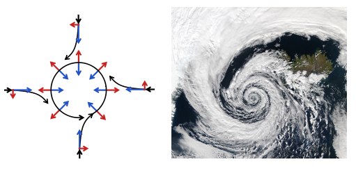
Reading
Read the link below.
- Coriolis Effect. [82] Thinking about Hadley circulation (and the image above), why does a north wind (i.e., a wind from the north) in the Northern hemisphere, such as in a Hadley Cell, blow toward the southwest?
Ekman Transport Water in the ocean can be divided roughly into three regions based on density: surface water, the pycnocline, and deep water. The pycnocline (also called the thermocline or halocline: recall that seawater density (pycno) is determined by temperature (thermo) and salinity (halo). Winds drive surface currents in the ocean, and these currents are effected by the Coriolis effect. But surface flow causes motion in the water below, so things get a bit more complicated. The physical properties of Surface Waters vary smoothly from the ocean surface to the pycnocline, but for the purposes of this discussion, it's useful to imagine that the surface zone is composed of several layers of water. The top-most layer is driven by wind. Motion in this layer drives flow in the layer below, and so on, such that wind driven motion at the top, ultimately, drives flow in all of the layers below. Now here's the complication: each one of our 'layers' is influenced by the Coriolis effect. This sets up a spiral, with motion in each successively deeper layer bent somewhat to the right (in the Northern Hemisphere) relative to the forcing from above.
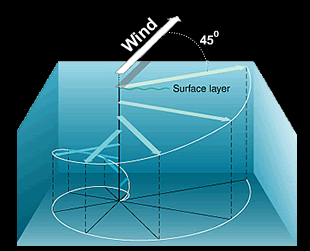
Read more about Ekman Transport here [83]
Ocean Circulation: Surface Water and Deep Water
Global ocean currents and thermohaline circulation
Reading assignment
Read the link below.
- Broecker, GSA today [84] What If the Conveyor Were to Shut Down? Reflections on a Possible Outcome of the Great Global Experiment
Recall from Lesson 3 that water density increases with increasing salinity and decreasing temperature. Water density varies throughout the ocean and the water at the bottom of the ocean is densest, of course. Ocean-atmosphere interactions have important implications for global ocean currents. For example, think about what would happen if a large scale surface current continually lost heat. The colder it got the denser the water would be, and eventually that water would become dense enough to sink, and become deep water. Now lets add in evaporation. Imagine that water was continually evaporated from our surface current. This would make it saltier, which would increase the density. Eventually, the density would increase enough for the water to sink and become deep water.
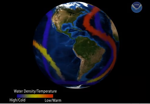
This is exactly what happens in the North Atlantic. But, if deep water forms in one place, then surface water has to form somewhere else; we can't push water into the deep ocean without something coming back to the surface, and in fact, surface water forms in various places in the ocean.
Look at the image above, and then back at the figure at the top of page 1 of this lesson. On page 1, the arrows are red for surface currents and blue for deep currents. The colors are a bit hard for me to see, but note that in the North Atlantic, a surface current flows north and a deep current flows south. This means that deep water forms in the North Atlantic.
It's important to appreciate that any Figure drawn at this scale, the entire ocean, is approximate. Don't take everything you see in these figures as the gospel. For a different perspective, have a look at this animation. [85]
The figure below shows the general structure of water masses as a function of depth in the ocean.
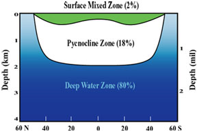
Activity 2
Why does surface water sink in the North Atlantic? Let's calculate the density differences between surface waters in the tropics vs. where deep water forms in the north.
Go to the Windows to the Universe [87] is web site and read the information there (under: Density of Ocean Water)
Then click on the links in the second paragraph for ("the temperature [88] of the water and the salinity of the water [89]....")
Use those images to determine Temperature and Salinity in the North Atlantic off the coast of Florida and off the coast of Ireland.
For temperature, you'll need to click on the link for "Sea Surface Temperature Image [90]," which is under the heading "Related Links." If you have trouble finding it, click here [88]
For salinity, you can just click on "the salinity of the water" and then on the map at the top of the page.
The colors are a bit tricky to distinguish, but do your best and report the values you chose.
- Calculate the density of the water masses off the coast of Florida and off the coast of Ireland. Make sure to record your values for temperature and salinity. You can use the Ocean Water Density Calculator [91] for the density calculation
- Comment. Is this about what you expected? How are water densities normally determined in the ocean?
Submitting your work
Please put your answers in a file and drop that in the dropbox for Lesson 4, Activity 2 on Canvas.
Save your document as either a Microsoft Word or PDF file in the following format:
L4_Activity2_AccessAccountID_LastName.doc (or .pages or .pdf)
For example, student Elvis Aaron Presley's file would be named "L4_Activity2_eap1_presley.doc".
Grading criteria
See the grading rubric [12] for specifics on how this assignment will be graded.
Gyres and Surface Currents
The global pattern of winds together with the Coriolis Effect and Ekman Transport produce large-scale currents in the world ocean. Ocean surface currents organize into Gyres that are characterized by circulation at the scale of the ocean basin. The figure below shows the basic pattern. Note that gyres circulate clockwise in the northern Hemisphere and counter-clockwise in the Southern Hemisphere.
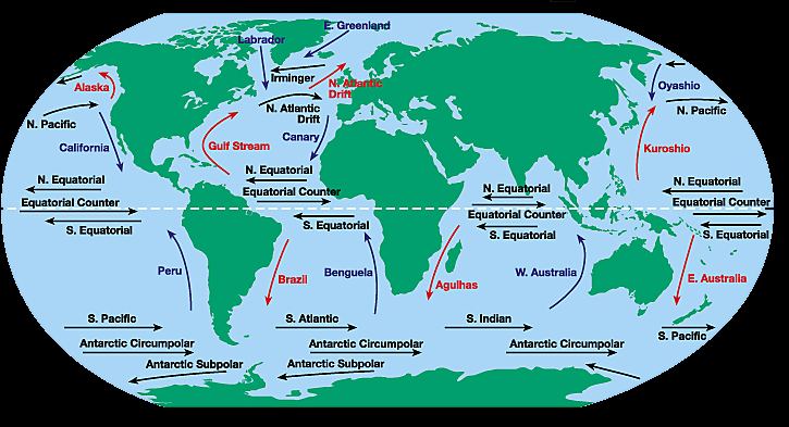
The influence of the Coriolis effect on ocean currents increases with increasing latitude, so the equatorial currents are similar in each ocean basin, although their flow direction (east to west) is consistent with the sense of flow in the large-scale gyres within each ocean basin. But the variation of Coriolis forcing as a function of latitude has a pronounced affect on surface currents. The poleward currents on the Western side of each ocean basin are distinctly different from those on the Eastern side of the ocean basin.
Western Boundary Currents are swift, narrow and deep relative to Eastern Boundary Currents, which are slower, broader and shallower than WBC's. Western Boundary Currents tend to carry heat from the equator poleward, so think back to where we started in this Lesson; everything is driven by differential solar heating. The excess heat received in the equatorial regions drives everything, including the strong Western Boundary Currents such as the familiar Gulf Stream and the East Australian Current (from Finding Nemo fame).
The figure below shows surface current information for the North Atlantic. The color scale is flow velocity in m/s, and the arrow along the bottom shows a 1 m/s scale bar (vector). Note the narrowness of the Gulf Stream.
Look here for more info on the Gulf Stream. [92]
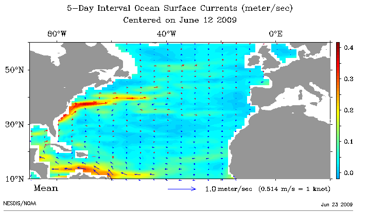
Activity 3
Let's make our own maps and use them to calculate some things about heat transport. For this activity we will use ESR (Earth and Space Research) out of Seattle, WA. They have great research projects like OSCAR (Ocean Surface Current Analyses Real-Time) which suites our purposes nicely. Let's visit them HERE [93]. There's some good background information about OSCAR there, but we will be using the link "OSCAR on SOTO", with SOTO standing for "State of the Ocean". Once you click on "OSCAR on SOTO", you will open up a really cool interactive map. I encourage you to play around with it for a bit to see what kind of data it is capable of conveying (we could have used this for our density calculations for Activity 2!) Once you're done playing, check out "Ocean Current Speed", but then settle on "Ocean Current Vectors".
->Note: This web site is mostly gone. Some of it is available here: https://www.esr.org/research/oscar/overview/ [94]
- Make and save (using "Grab" on a Mac or another print-screen application) a few maps of surface currents where you look at seasonal variations as well as flow directions and the basic pattern of ocean-basin scale gyres.
- Choose your favorite map and tell me why you chose it in a few sentences. What did you learn from it? Put your map in a file, along with your comments.
- And now for a couple of calculations.
- Calculate an estimate of the volume of water that flowed poleward in the Gulf Stream during all of June 2016.
- Calculate an estimate of how much heat was transported by the Gulf Stream in June 2016 (You can choose to estimate sensible heat and/or latent heat)
There are multiple ways one can do these, just make sure I can follow your train of thought through each/both. Your calculations should:
- incorporate the max velocity of the Gulf Stream from June 2016
- assume that the depth of the current is 1 km
- estimate the width of the Gulf Stream from your map
- use OSCAR to find temperature estimates
Submitting your work
Please put your answers in a file and drop that in the dropbox for Activity 3 on Canvas.
Save your document as either a Microsoft Word or PDF file in the following format:
L4_Activity3_AccessAccountID_LastName.doc (or .pages or .pdf)
For example, student Elvis Aaron Presley's file would be named "L4_Activity3_eap1_presley.doc".
Grading criteria
See the grading rubric [12] for specifics on how this assignment will be graded.
Additional Resources
Want to explore these topics more? Here are some resources that might interest you.
Various Web site with links to resources aimed at teachers and students:
- General Oceanographic Data in a form that can be used to make maps and plots [95]
- University Corporation for Atmospheric Research (UCAR) [96] Note the Teacher Resources linked at the top of the page
- NASA Earth Science satellite [97]: Hover on "NASA Science for" to select "Educators"
Tell us about it!
Have another Web site on this topic that you have found useful? Share it in the Comment area below!
Don't see the "Comment" area below? You need to be logged in to this site first! Do so by using the link at the top of the left-hand menu bar. Once you have logged in, you may need to refresh the page in order to see the comment area below.
Summary & Final Tasks
Reminder - Complete all of the lesson tasks!
You have finished Lesson 4. Double-check the list of requirements on the first page of this lesson ("Lesson 4" in the menu bar) to make sure you have completed all of the activities listed there before beginning the next lesson.
Once you've completed all lesson tasks, make sure you enter the "Teaching and Learning" discussion in Canvas and tell us how you would teach a topic from this lesson in your own classroom
Tell us about it!
If you have anything you'd like to comment on, or add to, the lesson materials, feel free to post your thoughts below. For example, what did you have the most trouble with in this lesson? Was there anything useful here that you'd like to try in your own classroom?
Don't see the "Comment" area below? You need to be logged in to this site first! Do so by using the link at the top of the left-hand menu bar. Once you have logged in, you may need to refresh the page in order to see the comment area below.
Lesson 5
Lesson 5 Introduction
The Sea is Rising, the Sea is Rising
About Lesson 5
We will complete Lesson 5 in one week. The topic is vast, and perhaps worthy of a course in itself: climate change and its impact on sea level and the coastal zone. Our plan is to first study the methods, data, and observations related to past, present and future sea level change, then evaluate the impact of sea level change on the coastal zone. We will examine the interplay of data and models as well --inasmuch as future predictions are model based. Along the way, you will learn a little something about coastal evolution. Critical reading and evaluation of data are again key components of the Lesson. As you might surmise, future sea level rise is a controversial topic. We'll have some fun with the blogosphere and media distortion of scientific results.
What will we learn in Lesson 5?
By the end of Lesson 5, you should be able to:
- Explain the implications of global warming for sea level change
- Discuss the components of predicted future sea level rise
- Outline the impacts of sea level rise on the coastal zone
- Explain why beaches are dynamic features subject to continual change.
- Explain the origin of coastal estuaries and their history over the past 18 thousand years
- Relate the history of climate, continental ice sheets, and sea level of the past
What is due for Lesson 5?
As you work your way through these online materials for Lesson 5, you will encounter additional reading assignments and hands-on exercises and activities. The chart below provides an overview of the requirements for Lesson 5. For assignment details, refer to the lesson page noted.
| REQUIREMENT | LOCATION | SUBMITTED FOR GRADING? |
|---|---|---|
| Reading: Sea Level Rise, After the Ice Melted and Today | page 1 | |
|
Reading: IPCC Report: Observations: Oceanic Climate Change and Sea Level (this is a biggie!) Activity 1: Questions regarding sea level mechanisms and timing |
page 2 Canvas |
Essential Background Reading Yes, Canvas Dropbox |
|
Reading: "Birth of the modern Chesapeake Bay estuary" Activity 2: Questions regarding methods and implications |
page 4 Canvas |
Yes, Canvas Dropbox |
Questions?
Post them to our Questions discussion forum on Canvas or get in touch by email.
Buying Beach Property?
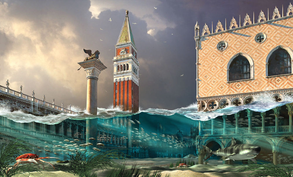
Yes, here is an essential question. Perhaps today's economy is not encouraging, so none of you are rushing out to purchase that beachfront house for the summer. But, let's assume that you have a cool million (or two) dollars languishing in your accounts--perhaps Bernard Madoff has just provided you a return on your investment! Would you go to your favorite coastal area, engage a real estate agent, and put in a bid for one of the many properties now available? Remember, buying when the market is down can make for good investments. Or would it in this case? The question is "what would you look for in a coastal property?"
Rather than answering that directly, let's embark on a consideration of the controversial topics of global climate change and resulting sea level change. Perhaps, after a reasonably intensive study of controls on sea level and predictions for the future, you will get cold feet on the coastal property purchase. Let's hope that it's not because you are standing inches deep in cold seawater in your living room! This fanciful artist's conception of Venice after a meter of sea level rise is not so far from reality. Engineers are, as we speak, planning an elaborate system of gates to prevent flooding of Venice while still allowing seawater to cycle through the adjacent wetland estuaries.
Reading--for an overview of global sea level change over the past 18 thousand years or so
Click on the links below.
T [98]he Great Ice Meltdown and Rising Seas: Lessons for Tomorrow [99] By Vivien Gornitz — June 2012
Why is an understanding of future sea level so critical? It's the economy, it lives in the balance...! Think about the implications of meters of sea level rise in a short period of time. According to modeling studies, a category three hurricane (not the most severe by any means), given a certain critical storm track to the west of Manhattan, could create a storm-surge (more on this in a later lesson) of up to 6 meters at JFK Airport, 7 meters at the Lincoln Tunnel entrance, 8 meters at the Battery, and 5 meters at La Guardia Airport. The numbers could be larger if the storm passage coincides with high tide and if one considers the height of waves riding on the surge. What if sea level were, on average, a meter or two higher? Catastrophic flooding, loss of property, life and enormous cleanup costs. Certainly, hurricanes have affected New York City in the past. One made landfall at Jamaica Bay on Sept. 3, 1821 with a 13-foot storm surge, causing widespread flooding in lower Manhattan. The "Great Hurricane of 1938," [100] a category three storm, tracked across central Long Island and southern New England on Sept. 21, 1938. The storm pushed a 25-35 foot high wall of water ahead of it, sweeping away protective barrier dunes and buildings. Some 700 people lost their lives during this storm. Things could be worse with any rise in sea level. The image below projects flooding associated with a Category 3 hurricane, as described above, with projections for additional flooding anticipated with given rises in sea level through 2050. Looks as though these "experts" might expect as much as 47 cm rise in the next 40 years. Hmmm, that's just over 1 mm per year. What is the present rate of rise? Is it expected to slow? On to the next phase of this lesson.
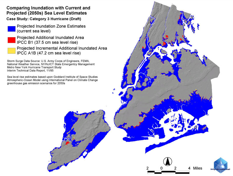
The Sea Also Rises--global change!
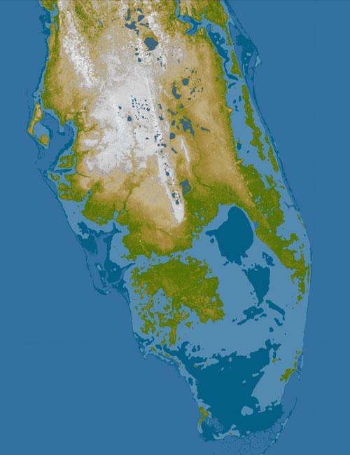
So, here is the (late?) great state of Florida flooded by a 5-meter rise in sea level (dark blue) and a 10-meter rise (light blue). Yes, far in the future, but not beyond imagination should, for example, the Greenland ice sheet completely melt back. Miami is gone, Tampa is gone...At what cost? When you take a look at a map of elevations around Miami, for example, you find that much development has occurred at heights above sea level of only 1 meter or so (see next chapter). Amazing! Could we ever do anything to save this region--short of building an elaborate set of dikes (like those protecting New Orleans today!) or somehow reversing the effects of global warming? What's going to happen to the folks in Holland?
Sea level changes on a global, as well as local, basis because of a number of factors. We are presently most concerned with rising sea level that results primarily from warming of seawater (why?), melting of continental glaciers and ice sheets (but not sea ice. Why?). How do we know that sea level has changed in the past, and how do we monitor sea level change at present?
Reading 2
Time to delve into something you've certainly seen in the news -- the well-known IPCC (Intergovernmental Panel on Climate Change) Report. This section of Working Group 1 discusses sea level change related to climate change. This is a "consensus" report from numerous scientists--experts in their fields. We're going to look mainly at the most recent Report (Fifth Assessment Report, AR5; 2013) and you might also want to look briefly at the 2007 IPCC Report.
You can find the full set of reports on the ipcc [101] website [101].
You will read Sections of Chapter 13, including the Executive Summary and Section 13.1 on Sea Level. You should also scan over other parts of Chapter 13, to get a sense of the overall content. This will provide an essential background in preparation for the first activity, so read carefully and make sure you understand the data, techniques and concepts. Feel free to post comments/questions below to the class with questions if there is something you do not understand.
When you are finished reading, you will go on to the next part in this Lesson to begin Activity 1.
Sea Level--what do we know about the past and future?
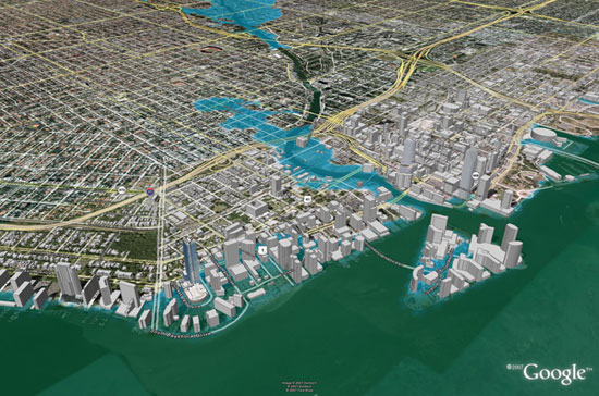
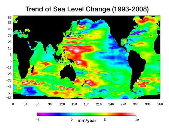
Activity 1
After reading the assigned articles and examining the figures above, answer the following questions. You may simply provide a list of elements, when appropriate. Elaborate if you like.
- How much sea level rise has occurred since about 18 thousand years ago and why (generally)?
- How do geologists estimate sea level history, at least for the last glacial through the Holocene (last 18 thousand years)?
- What methods are used to estimate rates of change of sea level at present and in the historical past? Provide an estimate of their accuracy.
- What are the major components of present sea level rise and their relative importance?
- In Figure 2 (above), why is there so much noise about the smoothed curve?
- In Figure 3, why do certain anomalies occur (explain in terms of circulation, winds, etc.--use principles from Lesson 4)?
- explain the large area of red to white color in the western Pacific on each side of the Equator
- explain the large area of light blue to dark blue in the eastern Pacific straddling the Equator
- speculate about the origin of the swath of blue to magenta projecting to the northeast from the margin of the eastern U.S.
- What is the "best" estimate as to the amount of sea level rise that will occur in the next half century? Why did you choose this number? What assumptions are you making when you state a number such as this? Provide an estimate of uncertainty based on the assumptions. Do you believe that this will come to pass?
- Think about the IPCC Report that you read. It represents a "scientific consensus." What does "consensus" mean in this regard? Do you view this term as controversial? Just because the "majority" of scientists accept this concept of global warming and sea level change, should we base our present and future actions on this hypothesis? Why or why not?
Submitting your work
Please put your answers in a file and drop that in the dropbox on Canvas.
Save your document as either a Microsoft Word or PDF file in the following format:
L5_Activity1_AccessAccountID_LastName.doc (or .pages or .pdf)
For example, student Elvis Aaron Presley's file would be named "L5_Activity1_eap1_presley.doc".
Grading criteria
See the grading rubric [12] for specifics on how this assignment will be graded.
Not All Sea Level Change is Bad (or Is It?)
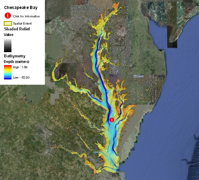
You can use Google Earth to explore your own digital map of water depths like the one above. Just download a file at NOAA's NCEI Bathymetry [104] site and, once downloaded, select the ".kmz" file. Files are quite large, but very elucidating (try to find something near your house or favorite beach!).
Note the deepest value of nearly 53 meters in the estuary above. Why do the deeper channels tend to hug the east side of the estuary? Is this Coriolis?
In this portion of Lesson 5, we will examine one role of sea level rise in coastal evolution--that of the formation of estuaries. Of course, estuaries are an important feature of the coastal region because they provide water routes to inland regions for shipping, defense, etc., and because they are typically nurseries for the larvae and immature stages of many marine organisms as well as being important fisheries. In this course we will concentrate on the Chesapeake Bay estuary because of its proximity to most of the class and importance to the economy of the mid-Atlantic region. Those in University Park, PA have a direct connection to the Chesapeake because they live in the Susquehanna River watershed which ultimately dumps into the Chesapeake Bay. We'll begin here with a study of the formation of this estuary, and in subsequent lessons we will explore the ecosystem itself and the problems it faces now.
Reading
Click on the links below to access a scientific article on the origin of Chesapeake Bay. Read this paper and think about the evidence that these scientists use to reconstruct the early history of this estuary and the timing and impact of sea level changes. Note the importance of the 8.2 thousand year "event."
- Bratton et al., 2003 [105]
Activity 2: Formation of the Chesapeake Bay Estuary
Let's outline some aspects of the work of a sedimentary geologist who is trying to reconstruct the timing and early history of an estuary. Answer the questions below to provide an overview of their approach and methods. Again, for some questions a short answer or list will suffice, but support your conclusion with further discussion if appropriate. Submit your ms word or pdf document as outlined below and drop into the Canvas dropbox for Lesson 5.
- What technique(s) allows the authors to establish absolute ages for the sedimentary layers in the estuary?
- Why is the estuary so deep? (e.g., what created the estuary morphology originally, and in response to what?)
- What is the most likely age of the establishment of the Chesapeake Bay estuary? What caused this event? (think back to your earlier reading on the origin of certain sea level changes in the past 18 thousand years).
- What evidence did the authors use to demonstrate that this was truly an "estuary"?
- How did the authors reconstruct sea level history at Site 5? (see Fig. 4 in the Bratton article)
- If the deepest part of Chesapeake Bay is around 53 meters, does this fit with the timing for flooding of the estuary by sea level rise argued in the Bratton et al. paper? (hint: examine an illustration for the history of sea level over the past 18 thousand years in one of the first two papers assigned for this lesson). If not, how could this discrepancy be explained?
Submitting your work
Save your document as either a Microsoft Word or PDF file in the following format:
L5_Activity2_AccessAccountID_LastName.doc (or .pages or .pdf)
For example, student Elvis Aaron Presley's file would be named "L5_Activity2_eap1_presley.doc".
Grading criteria
See the grading rubric [12] for specifics on how this assignment will be graded.
The Sea Also Rises--or Does It?
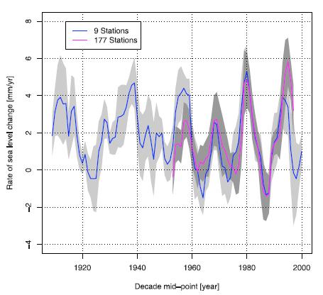
Let's evaluate some of the data sets required to establish the history of sea level changes. This history can provide a perspective on more recent rates of change. Inasmuch as it is our goal to encourage you and your students to critically evaluate scientific hypotheses and data, this is another in a series of issues that deserves deeper study. In particular, this is an opportunity to see how the media respond to various issues and how individuals might distort conclusions of scientific papers, or selectively extract certain data or plots, to further their own objectives. It will not surprise you to find that there are skeptics regarding the predictions of the IPCC Report and others. We will examine some of them and attempt to analyze their methods and misstatements or misleading conclusions. You can have some fun with this and perhaps think about how it would tie in with teaching goals.
Reading
This is the scientific paper published in 2007 by S.J. Holgate, a reputable scientist studying sea level changes at the Proudman Oceanographic Laboratory, Liverpool, UK (wonder if he listens to "Yellow Submarine" when he writes his papers?). The paper is a critical evaluation of tide gauge data used in reconstructing sea level history. You will need to read this paper to understand how tide gauges are used and their strengths and weaknesses. The paper also emphasizes spatial statistics, which are an important consideration in global reconstructions.
- Holgate, 2007 [106]
Consequences of Sea Level Rise
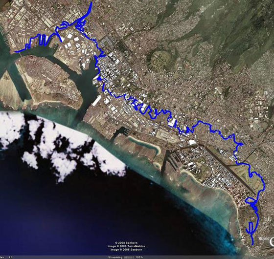
Think again about the economic and human consequences of sea level rise. Developed areas would be flooded at great cost, or, we would have to spend inordinate amounts of "public" money to protect them. In areas such as Bangaladesh, sea level rise would wipe out agricultural production and cause huge loss of life (which already occurs during cyclones in the Indian Ocean).
Sea level rise will inexorably cause the coastal zone to "step back" just as has occurred over the past 18 thousand years as wave attack erodes cliffs and moves sand from beaches farther onshore and offshore. Our favorite barrier island beaches will evolve, but the houses on them will be destroyed or moved back at great cost.
Additional Resources
Here are several more web sites. We highly recommend the Real Climate site as a resource to understand the nature of arguments for and against human-induced global warming and its consequences. This is a moderated site, but allows dissenting viewpoints. Very balanced.
- The Real Climate page (excellent discussions, pro and con) [107]
- Sea Change: How High Will the Sea Rise? [108]
- NOVA - "Mountain of Ice: If the Ice Melts" [109]
Tell us about it!
Have another reading or Web site on these topics that you have found useful? Share it in the Comment area below!
Summary & Final Tasks
Reminder - Complete all of the lesson tasks!
You have finished Lesson 5. Double-check the list of requirements on the Lesson 5 Overview page to make sure you have completed all of the activities listed there before beginning the next lesson.
Once you've completed all lesson tasks, make sure you enter the "Teaching and Learning" discussion in Canvas and tell us how you would teach a topic from this lesson in your own classroom
Tell us about it!
If you have anything you'd like to comment on, or add to, the lesson materials, feel free to post your thoughts below. For example, what did you have the most trouble with in this lesson? Was there anything useful here that you'd like to try in your own classroom? Is climate change a topic you and your students are interested in? Do your students have much interest in or opinions about the politics/science of global climate change?
Lesson 6
Lesson 6 Introduction
Tides
About Lesson 6
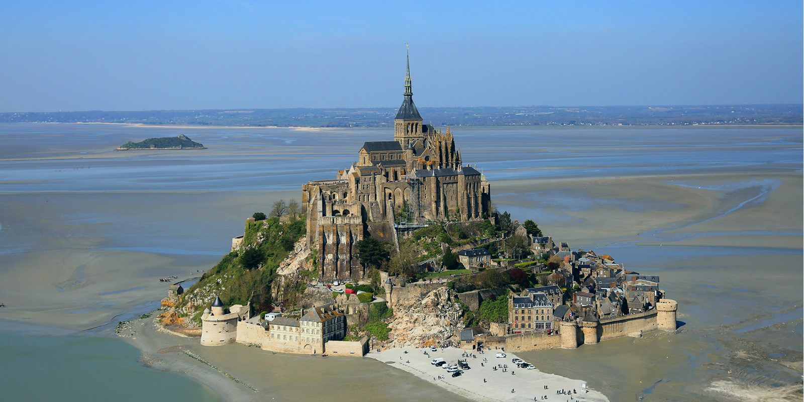
In this lesson, we will focus on the origin of ocean tides. We'll look at things in terms of an equilibrium (simple) model and in terms of a dynamic model of tides that takes into account factors such as ocean basin geometry and coastlines.
By the end of this lesson you should be able to explain the role of gravity, inertia, and rotating reference frames in determining tides. You should be able to describe why, in the equilibrium theory of tides, there are two tidal bulges on Earth; one that is roughly under the moon and one that is roughly antipodal to that.
The concept of Amphidromic points is important in understanding tidal circulation in the oceans. You should be able to describe how amphidromic circulation works, including co-tidal lines, co-range lines, and the role of the Coriolis effect.
What will we learn in Lesson 6?
By the end of Lesson 6, you should be able to:
- Describe how the Earth-moon system rotates during a lunar month, and why the focal point is within but not at the center of Earth.
- Explain the role of gravity, inertia, and rotating reference frames in determining tides.
- Describe why semi-diurnal tides involve two high tides and two low tides at a given location during roughly a 24 hr. and 50 min period.
- Describe why the concept of Amphidromic points is important in understanding tidal circulation in the oceans.
- Describe how amphidromic circulation works, including co-tidal lines, co-range lines, and the role of the Coriolis effect..
- Use on-line resources to construct maps of ocean temperature and salinity
What is due for Lesson 6?
The chart below provides an overview of the requirements for Lesson 6. For assignment details, refer to the lesson page noted. See the Course Schedule (located in the Resources menu) for assignment due dates.
| REQUIREMENT | LOCATION | SUBMITTED FOR GRADING? |
|---|---|---|
| Read the information on the next page and then complete the Tides Activity on Canvas Prepare for the End-of-unit Quiz, on Canvas |
Canvas | Yes. Complete Tides Activity on Canvas under Lesson 6 |
Questions?
If you have any questions, please post them to our Questions? discussion forum (not e-mail), located under the Communicate tab in Canvas. I will check that discussion forum daily to respond. While you are there, feel free to post your own responses if you, too, are able to help out a classmate.
Tides in two easy pieces

Let's start with the equilibrium theory of tides, and let's ignore the Sun for a moment. The moon accounts for about 2/3rd of the Ocean tides anyway, so we'll have almost everything. Also, the concepts we develop for the moon apply equally to the Sun-Earth system.
There are a few simple things to keep straight with tides. The first involves the assumptions we make for the equilibrium theory, when trying to show the simplest way to understand things. In this view, there are two ocean tidal bulges on opposite sides of Earth. One is under the moon and the other is opposite to that. The one under the moon is thought of as 'gravitational.' Newton told us that every point mass in the universe is attracted to every other mass, via gravity, with resulting force proportional to the product of the masses divided by the square of the distance between the masses. He also showed that a spherical body can be represented as a point mass at its center. Tidal forcing is proportional to the ratio of mass over distance cubed.
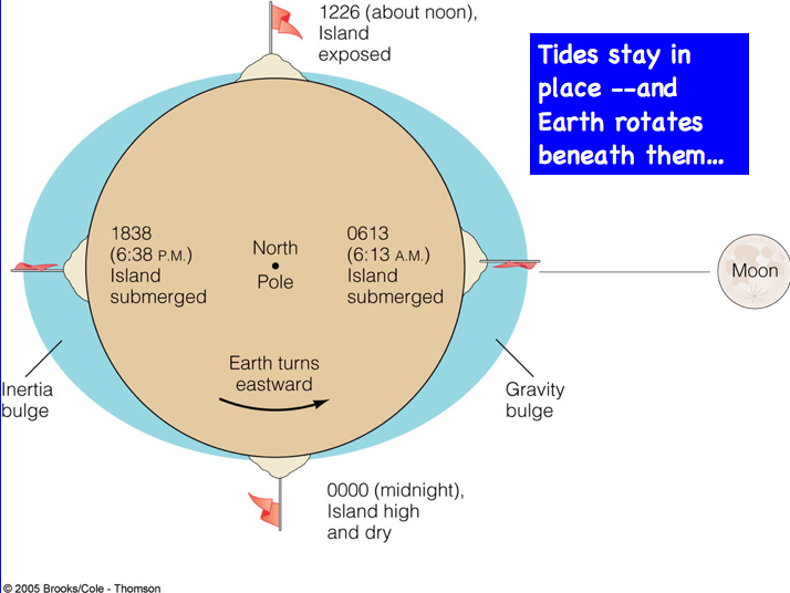
So, in our simple picture, the tidal bulge under the moon is produced by gravitational attraction between water molecules in the ocean and the moon. Now, what about the other bulge? Well, you have to think about inertia and what happens when masses rotate around a point. One relevant common experience is that of swinging a bucket of water around with your arm. The rotation produces a 'centrifugal force' that holds the water in the bucket, even when it's overhead and gravity is trying to make the water fall out of the bucket. The same thing happens during a lunar month as the Earth-moon system rotates. The moon orbits Earth, but the rotation axis for this orbit is not at Earth's center. Both the moon and Earth move during the roughly 28 day period it takes for the orbit, and because of this, water in the ocean is thrown to the outside, the same as the water in your bucket. The tidal bulge on the opposite side of Earth from the moon is produced by this inertial effect, referred to as centrifugal force.
There are some simplification here that we need to be clear about, but before we do that, let's follow through and see the logical conclusions of our model. We have two ocean tidal bulges. During a 24-hr. period, the moon is roughly stationary with respect to our simple diagram. This means that our tidal bulges are roughly stationary, and if that is true, it means that a point on Earth's surface rotates under each of these bulges and under each of the 'troughs' of low water level that are produced by the ocean water that was attracted to the moon gravitationally and thrown off the side of Earth, inertially, respectively, to produce high tides. The water to produce the high tides, associated with the tidal bulges, has to come from somewhere, and this means that sea level is lower (low tide) at locations between the high tides. Let's make things as simple as possible and imagine a situation where the moon is more or less directly over the equator, with one tidal bulge centered on the Prime Meridian. Then the other tidal bulge is centered on 180 deg. longitude. Imagine we are on the beach in Ecuador, and lets see what happens. During a 24-hour period, we'll have two high tides and two low tides, as our coast rotates under a tidal bulge (high tide) then a trough (low tide) then the other bulge (high tide) and the other trough (low tide). This situation is referred to as semi-diurnal tides and this type of tidal situation is the most common along coasts world wide. Now, let's think a bit more carefully about our assumptions and the equilibrium theory.
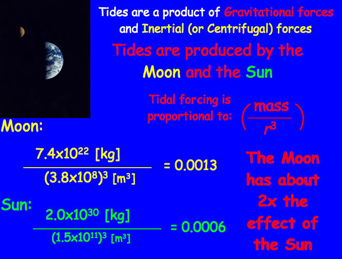
Tides are a product of Gravitational forces and Inertial (or Centrifugal) forces. Tides are produced by the Moon and the Sun.
Tidal forcing is proportional to:
Moon:
Sun:
The Moon has about 2x the effect of the sun.
First, let's realize that both tidal bulges in our model are produced by gravity in a rotating reference frame. The moon is in orbit around Earth due to gravitational attraction. The Earth-moon system rotates around it's center of mass, which is located at a point within Earth, but not at Earth's center. How would you go about calculating the location of the center of mass? So, when you see a diagram of Earth with two bulges, one labeled gravitational and one labeled 'centrifugal,' you can smirk and think about why it's not strictly correct; the 'centrifugal force' is actually produced by gravity and inertia. Earth is rotating around the center-of-mass in a 28 day period, and ocean water is thrown off toward the outside (think of your bucket of water.)
Ok, is that all? Well, think about the water in the Atlantic ocean and then think about a place like, say, Daytona Beach. What if the moon is actually over the longitude of Kansas? Hmmm, where are the tidal bulges? For the Atlantic, one bulge might be toward the west coast of the ocean basin, but clearly the ocean tidal bulge is not over Kansas. Here's the problem with the equilibrium theory of tides: we ignore ocean basins and coastlines, and we just think in terms of an ocean that covers the entire Earth. Obviously, this isn't correct, but it allows us to make progress, so it's a good place to start. For now, we can envisage some islands that are scattered here and there, so as to have some point of reference for sea level and for reckoning high and low tide.
The equilibrium theory sounds far fetched (no ocean basins? no coast lines, humph) but when we get to the dynamic theory of tides, I think you'll see why we started simple. We're going to have to bring in Coriolis and other complicating factors. For now, let's take a couple more steps with the equilibrium theory. As we've already seen, it does a pretty good job of predicting semi-diurnal tides, which are the most commonly observed tides. What happens when the moon is not over the equator, and what about times when the moon is closer to Earth (Perigee ~ 0.36x10^6 km) or farther from Earth (Apogee, ~ 0.4x10^6 km)? The moon's orbit around Earth is elliptical, so at certain times of the lunar month it will be closer to Earth. When the moon is closer to Earth, the 'gravitational' bulge is larger than when the moon is farther from Earth. Recall that the plane of the moon's orbit around Earth is generally not parallel to the equator and can be as much as 28.5 degrees. When the moon's declination is large, an interesting 12-hour asymmetry develops for semi-diurnal tides, and it's possible to understand it with the equilibrium theory of tides. The tidal bulges are positioned under the moon and antipodal to this point. Therefore, when a given location on Earth makes one revolution in a 24 hour period it experiences one high tide that is higher than the other and one lower low tide. Despite the success of the equilibrium theory of tides, at some point we have to admit that Earth is not covered by a single ocean.
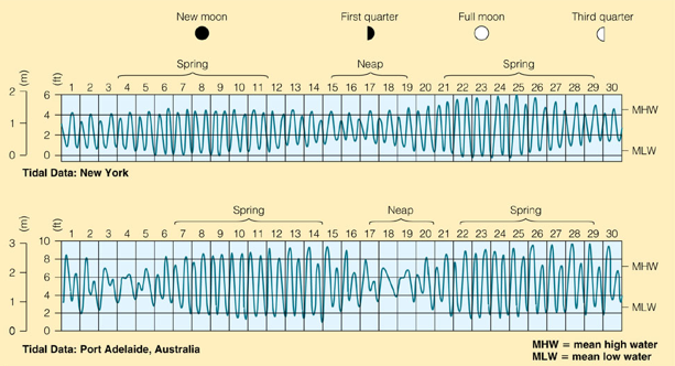
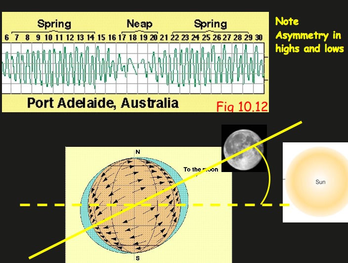
The dynamic theory of tides takes into account ocean basins of finite size and other complexities associated with coastlines. Many factors must be taken into account in order to accurately predict the tides in a given coastal setting. For example, the solid Earth experiences a tide --the amplitude of which can be 10 cm or more-- and the finite viscosity and flow properties of water need to be taken into account in order to predict resonance effects where water is flowing in and out of a restricted basin (e.g., the Bay of Fundy or the Gulf of Mexico.) The dynamic theory of tides is complex, but includes a simplifying concept know as amphidromic circulation. The idea is that tides can be thought of as shallow water waves that circulate around a point in the ocean, known as the amphidromic point. The tidal range is zero at the amphidromic point and increases with distance from this point, such that tidal range is maximum along the coast lines far from the amphidromic point (which is generally near the center of the ocean basin.) It's useful to think first in terms of a hypothetical ocean basin (we can assume it's square in map view) and then once we have the general picture down, to look at a real amphidromic circulation.
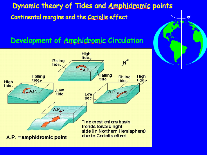
Amphidromic circulation stems from two basic effects. First, the water in a given ocean basin stays in that ocean basin. So when Earth spins under the tidal bulges, rather than the water staying in place as the Earth spins, as we assumed in the equilibrium theory, the water first builds against the west side of the ocean basin, and then sloshes back toward the center of the ocean as the continent spins under the moon, or antipodal to it. The water sloshes from West to East (think of a big basin of water that you tip from side to side --this is the scale that we are thinking in terms of for tides) but rather than going in a direct line, the motion is impacted by the Coriolis effect. In the Northern hemisphere it causes the wave to bend to the right, creating a counter-clockwise circulation, and it's the opposite in the Southern hemisphere. The tidal bulge sloshes from west to east, but ends up against the southern coast of our ocean basin. Then it sloshes back toward the center, from south to north, but it's bent to the right (Northern Hemisphere) and ends up against the East side of the ocean basin. In the Northern Hemisphere, this creates a ccw amphidromic circulation around the amphidromic point.
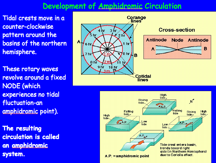
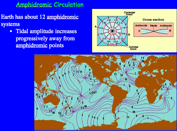
OK, that's it for Tides. Complete the activity on Canvas and you'll be in good shape.
Meantime, spend time on your projects and catch up with other work.
Recall: shallow water waves occur when water depth is less than roughly a factor of one half of the wavelength.
And, make plans to watch the next lunar eclipse.
A fun tool to find eclipses (lunar and solar) near you: Time and Date [111].
Once you've completed all lesson tasks, think about how you would teach a topic from this lesson in your own classroom; that might be a useful start for thinking about your Capstone Project for the course
Lesson 7
Lesson 7 Introduction
About Lesson 7
Time to consider the shallow-marine environment and the impact of human activities on the critters that live there. Yes, we want to inject a bit about marine biology and ecology into this course, so this is a beginning. In this Lesson we will explore "Dead Zones" and "Bleached Reefs" and evaluate their causes and consequences. We will cruise around a bit, spending some time in the Caribbean Sea on coral reefs, floating out the mouth of the Mississippi River to visit the "dead zone" along the coast of Louisiana, and then sailing up Chesapeake Bay to examine hypoxia there, and, finally, checking out "red tides" off the coast of Florida and Massachusetts. Actually, we'll visit the dead zones first and spend quite a bit of study on Chesapeake Bay. After all, if you like oysters, crabcakes, striped bass and the like you should be concerned about the health of that water body.
What will we learn in Lesson 7?
By the end of Lesson 7, you should be able to:
- Discuss the role of nutrients in production of marine phytoplankton
- Outline the impact of changes in dissolved oxygen in seawater on marine biotas.
- Outline and explain the causes of oxygen deficiency in marine environment
- Describe the circulation of a large estuary.
- Explain the nature and origins of red tides
- Describe the impacts of red tides on humans and marine organisms
- Outline elements of the ecology of modern coral reefs
- Identify disease and other issues that impact corals and reefs.
- Describe possible futures for coral reef systems.
What is due for Lesson 7?
As you work your way through these online materials for Lesson 7, you will encounter additional reading assignments and hands-on exercises and activities. The chart below provides an overview of the requirements for this Lesson. For assignment details, refer to the lesson page noted.
| REQUIREMENT | LOCATION | SUBMITTED FOR GRADING |
|---|---|---|
| Activity 1: Chesapeake Bay hypoxia | page 3 | Yes- Word file with answers to queries, post blog to Canvas discussion |
| Activity 2: Dead zones | page 4 | Yes- Word file with answers to queries. |
| Activity 3: Ocean Acidification | page 8 | Yes - letter to humans posted to Canvas discussion |
Questions?
If you have any questions, please post them to our Questions? discussion forum (not e-mail), located under the Communicate tab in Canvas. I will check that discussion forum daily to respond. While you are there, feel free to post your own responses if you, too, are able to help out a classmate.
Marine Ecology: What Will the Future Bring?
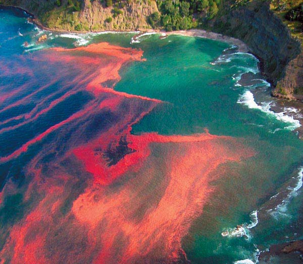
We could have subtitled this the "doom and gloom" lesson. Because, yes, it does seem that the future of the marine realm is troubled in a variety of ways. In thinking about the problems facing our oceans, one could consider this quote from Mahatma Gandhi..."you must not lose faith in humanity. Humanity is an ocean; if a few drops of the ocean are dirty, the ocean does not become dirty." This works on various levels, don't you think? We can have hope for the future...alas, more than a few drops of the ocean are dirty now, especially the coastal ocean. Humans have too long thought that "dilution is the solution" to waste products, and we have allowed too much of our waste to escape down rivers and through the atmosphere to accumulate in the ocean and in oceanic sediments. It would appear that we are beginning to pay the price for our profligacy and neglect. Can we make amends? We hope so, right? In educating our youth we do not want to leave them with the impression that "all is lost," "we're hosed," the "system is kaput," etc. On the other hand, it is essential that everyone understand what is going on and what may come in the future.
What are the major environmentally related issues facing the ocean today?
- many coral reefs are affected by various bacterial and viral diseases that appear to have spread over the past decade or so, impacted by warming of waters (global warming?) beyond the tolerance of corals, which may be the major cause of "bleaching," and, a potential threat to their ability to form skeletons because of the buildup of carbon dioxide in the atmosphere and ocean.
- "red tides", (sometimes referred to as HABs--harmful algal blooms) dense blooms (not in the flowering sense, but in numbers) of toxic phytoplankton (near surface-dwelling, single-celled photosynthetic floating organisms) are appearing in estuaries, bays and coastal regions. These organisms, typically dinoflagellates, secrete neurotoxins that can accumulate in certain marine organisms (e.g., raw oysters! mmmmmm!) that some humans love to eat, and will cause paralysis or death if consumed. In fact, crabbing season (a San Francisco tradition in December) was canceled in 2015 due to HABs!) They also cause other problems for the normal marine biota that we will examine later. Red tides have been known for decades, but their frequency and distribution is increasing rapidly.
- "dead zones" and "hypoxia," regions of estuaries, bays and even the open continental shelves that suffer from oxygen deficiencies. Extreme low oxygen concentrations eliminate benthic organisms (e.g. clams, scallops) and reduce habitat for oysters, crabs, fish and the like. These "dead zones" are likely caused by a surfeit of nutrients, excessive plankton blooms, restricted mixing of surface and deeper waters, and high rates of oxygen consumption by bacteria that break down the falling organic matter. These areas seem to be increasing in number and expanding.
- oil spills and leakage that harms waterfowl and marine mammals (e.g. the BP incident). We will not cover this issue in the course. Double-hulled oil transport vessels seem to be the main solution to this issue (that, or stop using oil and gas...?).
- overfishing and a "jellyfish ocean". This is discussed in the Lesson on fish and fisheries.
These issues (and their possible solutions) are covered in two relatively recent books using the theme "Ocean's End."
We recommend both: Ocean's End by Colin Woodward (2001) is a bit depressing but graphic, whereas Defying Ocean's End (2004) by Linda K. Glover, Sylvia A. Earle (a real force in marine science and diving), and Graeme Kelleher gives the "agenda" for approaching the problems. Also, visit the "Defying Ocean's End" [113] wikipage for other details and updates.
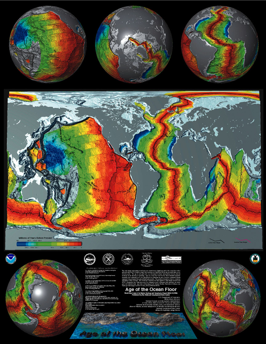
Let's jump right into the Chesapeake Bay story as an example of issue #3 (and #2 to some extent).
Is Chesapeake Bay Dying a Slow Death?

By way of introduction, please view the power point presentation [116] on the problem of dead zones, hypoxia, eutrophication and the health of Chesapeake Bay. Then go to the assignment below to flesh out your knowledge. If you're having trouble viewing the PowerPoint, try the PDF [117]. (admittedly, this ppt is a tad aged, but the trends stand and we will discuss updated data soon!)
We think that this is a great focus for teaching about the oceans, primarily for teachers in the northeastern US, because it is "local," has food chain connections, and involves so many aspects of physical oceanography, nutrients and primary production, marine animals, environmental issues, fisheries--you name it! However, we think that oceans on both coasts experience many of the things in this presentation, so don't despair if you're on the west coast...it's great for you, too! And, there are so many resources and data sets available for students to work with.
Activity 1
After reading the first assigned article (Brattonetal2003 [118]), which provides an historical overview of Chesapeake Bay hypoxia on the basis of the sedimentary record, and examining the power point presentation above, answer the following questions (in a file to be uploaded to the Canvas DropBox). You may simply provide a list of elements, when appropriate. Elaborate if you like.
- What factors contribute to hypoxia in Chesapeake Bay? How does each factor operate to exacerbate the major influence?
- Historically, when did hypoxia first develop in Chesapeake Bay? Was it extensive and when did it begin to more fully develop (see article by Bratton et al.)?
- What methods are used by "paleo-oceanographers" to reconstruct the history of hypoxia? What does each method or indicator really tell them? (again, reference the Bratton et al. paper)
- What are the consequences of Chesapeake Bay hypoxia? Be explicit regarding the many issues.
- What are the main things that need to be done to improve the "health" of Chesapeake Bay?
- Write a short summary of the current state of Chesapeake Bay. Emphasize the extent of improvements that have occurred, if any, over the past few years and the prospects for the near future. Assume that you are writing this for people in the Chesapeake Bay watershed. You might want to consult these sources for updated information on the state of the Bay. (here is the latest "bay barometer [119]" from The Chesapeake Bay Program [120]; you should also check out the Chesapeake Bay Foundation [121] website; each state also maintains a CB-oriented website. Maryland and Virginia are particularly good and those of us in California use The Bay Institute for all our bay health needs)
- Write a short summary of how would you appeal to the populace external to the Chesapeake Bay watershed? Why should they care about this issue.
Submitting your work
Please put your answers in a file and drop that in the dropbox on Canvas.
Save your document as either a Microsoft Word or PDF file in the following format:
L7_Activity1_AccessAccountID_LastName.doc (or .pages or .pdf)
For example, student Elvis Aaron Presley's file would be named "L7_Activity1_eap1_presley.doc".
Grading criteria
See the grading rubric [12] for specifics on how this assignment will be graded.
Dead Zones of the Gulf of Mexico and other Maladies
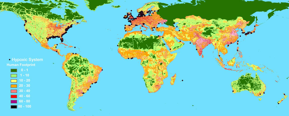
Ok, so far you know a bit about hypoxia and dead zones on the basis of your exploration of Chesapeake Bay. In this section, we will explore the Gulf of Mexico "dead zone" a bit more, with a short activity to follow. NOAA has its own website dedicated to monitoring Gulf of Mexico hypoxia. Head to NOAA [122]and peruse the linked documents and maps. Here's a website (NASA ocean color [123]) that shows satellite imagery of some representative zones with a bit of explanation. And this NOAA [124] website has an interesting historical focus and research plan, including "Public Comments" regarding policy issues (check them out--the public comment period closed in 1999, but some very interesting debate there). If you look these over carefully, you should be able to go to Activity 2. You will now be quite an authority on "dead zones."
Review
Spreading Dead Zones and Consequences for Marine Ecosystems [125]
Robert J. Diaz1* and Rutger Rosenberg2
Science 15 August 2008:
Vol. 321. no. 5891, pp. 926 - 929
DOI: 10.1126/science.1156401
Dead zones in the coastal oceans have spread exponentially since the 1960s and have serious consequences for ecosystem functioning. The formation of dead zones has been exacerbated by the increase in primary production and consequent worldwide coastal eutrophication fueled by river in runoff of fertilizers and the burning of fossil fuels. Enhanced primary production results in an accumulation of particulate organic matter, which encourages microbial activity and the consumption of dissolved oxygen in bottom waters. Deadzones have now been reported from more than 400 systems, affecting a total area of more than 245,000 square kilometers, and are probably a key stressor on marine ecosystems.
1 Virginia Institute of Marine Science, College of William and Mary, Gloucester Point, VA 23062, USA.
2 Department of Marine Ecology, University of Gothenburg, Kristineberg 566, 450 34 Fiskebckskil, Sweden.
Reading
This scientific paper, published in 2008 by Vaquer-Sunyer and Duarte in PNAS, suggests that the severity of hypoxia controls diversity of benthic marine organisms and that there are different thresholds for different groups (like we showed in the slideshow for CB at the beginning of this lesson). After reading this short but pithy paper, take on Activity 2.
Activity 2: Reading the Scientific Literature
Activity 2 should be submitted to the DropBox on Canvas
See the grading rubric [12] for specifics on how this assignment will be graded.
- You have read this PNAS paper. In your own words, summarize the principal points they made and their significance. Do this in less than 100 words.
- Next, answer the following questions
- What do the "L50" parameters mean and what is the "threshold" for low oxygen tolerance?
- Which organisms are most susceptible to oxygen deficiencies? Least?
- What strategies can different organisms use to cope with oxygen deficiency? Does this influence their susceptibility as listed in question #2?
- Provide a paragraph that briefly compares and contrasts the causes and effects of hypoxia in Chesapeake Bay with that in the Gulf of Mexico "dead zone."
Red Tides: Don't Eat Seafood in Months without an "R"?
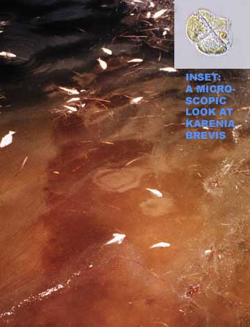
Have you ever been told "don't eat seafood in months without an "r"? As kids, many of us were told that but never really knew why. Turns out, that the summer months are typical "red tide" months and raw seafood consumption was not a good idea because of PSP (paralytic shellfish poisoning). In fact, California has a state law that allows substitution of punched "ray" fin for scallops in restaurants during those summer months without notifying the consumer for that reason.
Red Tides
Are "red tides" and PSP bad? Well, examine this map [127] and you will see that the incidence of PSP has spread considerably with red tides. Take about a half hour to pore over this fairly self-explanatory slideshow about plankton ecology and HABs (harmful algal blooms) [128]. The link will download a file: HABs.ppt. This should give you what you need to understand the food web discussion in Lesson 8, and all about the requirements of photosynthesis in the sea and why nutrients are important and, at times, problematic. Plankton may be responding to global change as indicated in this summary that appeared in Science [129]magazine.
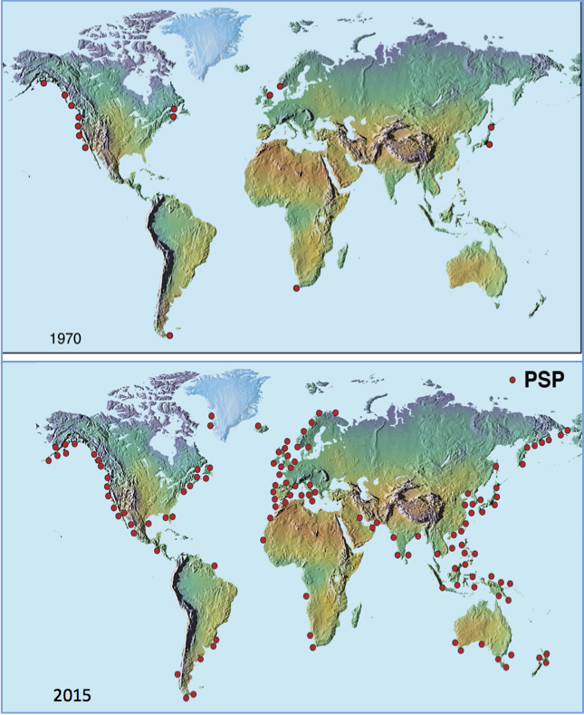
There are more resources on HABs on the last page of this Lesson. Any questions? Go on to Coral Reefs!
Health Care for Corals?
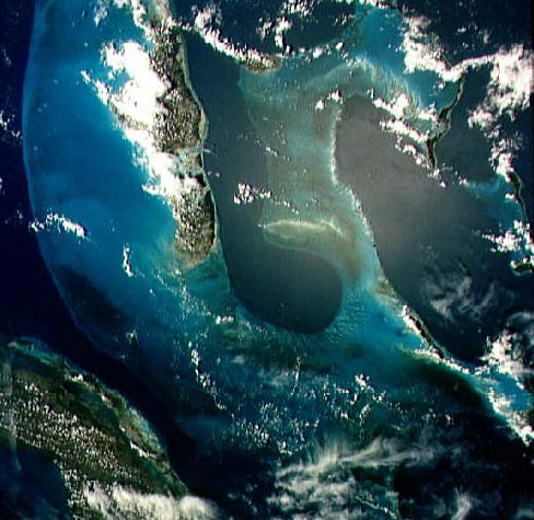
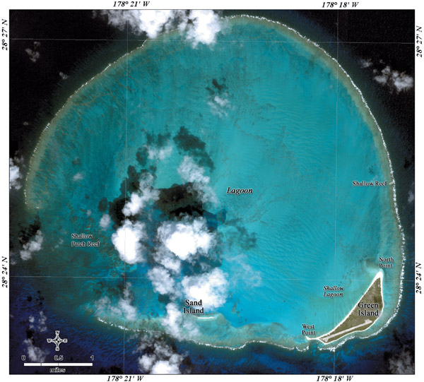
Coral reefs are widespread today in low latitude oceans where mean annual temperature and/or minimum temperatures at the sea surface (SST) are above 20°C. The coral platforms typically form fringing reefs and are barriers to wave energy. In the continental US, our only significant reefs are in the Florida Keys. Perhaps you have visited and snorkled on some of these reefs in Pennecamp State Park. The Hawaiian Island chain also hosts some spectacular reefs, which are, on some island margins, highly pristine.
But, as stated at the outset of this lesson, coral reefs nearly everywhere are imperiled, if not because of boats running aground and or anchoring on them then because of waters that are at times too warm and because of viral and bacterial diseases that are able to take advantage of these stressed organisms. In some cases, too much sediment and nutrients choke out corals and or promote overgrowth of green algae that block sunlight to the coral animals and their essential algal symbionts (stay tuned to learn a bit about these). These reefs are critical elements of the ecosystem, hosting a highly diverse animal and marine plant population as well as protecting adjacent coastal lagoons and and areas from erosion and damage by waves. The shallow oceans would seem sterile and, well, even ugly without them. Take a look at Figure 6-3, for example that shows a reef that is denuded due to disease and algal overgrowth.
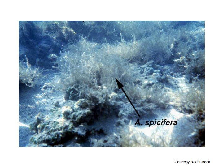
At any rate, before we go any farther, you should check out this short slideshow [130] that will familiarize you with general elements of coral reefs today. There are maps of their distribution and photographs of corals and coral diseases. We recommend that you check out a DVD of "The Blue Planet" [131] (also good for your regular dose of David Attenborough).
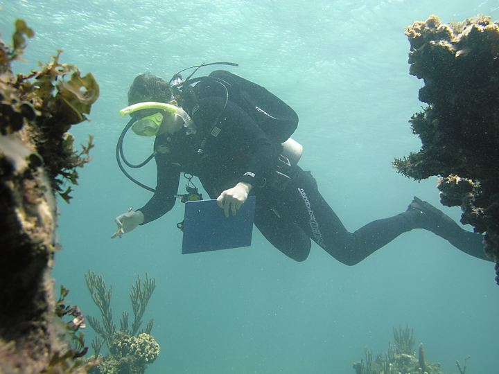
So, assuming you have looked at the slideshow as suggested, let's go on to the next section for some interesting (we hope) consideration of the interaction between atmospheric chemistry, the oceans and coral reefs. Another connection to "global warming" with a twist.
Another Big Whammy for Coral Reefs: Increasing Atmospheric Carbon Dioxide?
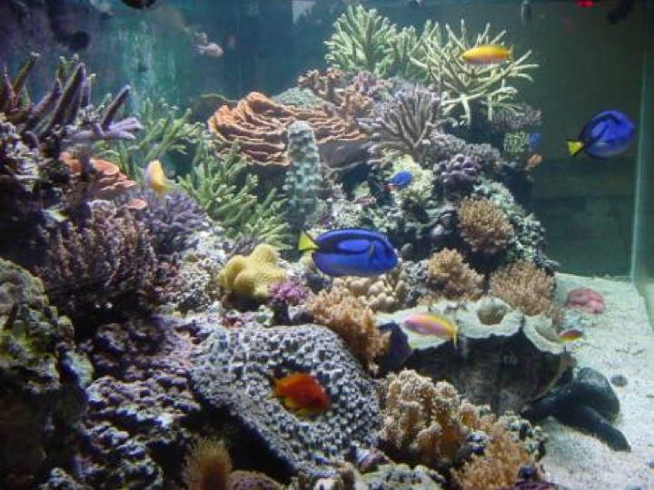
Yes, even at landlocked Penn State, we have a piece of shallow-marine environments, right in the midst of the bustle of the Hetzel Union Building (HUB) on campus. Thanks to the class of '99, a dedicated faculty member from Chemistry and a string of dedicated students this aquarium and its denizens continue to thrive. Here [132]is a brief article about the aquarium (2002) with pictures. One of the things learned in maintaining such small ecosystems is the need to buffer changes in certain chemical substrates, particularly dissolved carbon, pH and Calcium ions, all of which are essential to allowing corals to precipitate their aragonite (CaCO3) skeletons. The aquarium maintains a bed of granulated limestone through which fluids are circulated before they enter the tank. This allows some of the limestone to dissolve, if needed, contributing the essential Ca2+ and CO3-2 ions for incorporation by growing, skeletonizing corals. The chemical reaction would be:
Ca2+ + CO32- ----> CaCO3(s) (aragonite) (this reaction is, of course governed by a temperature-sensitive equilibrium "constant")
As you learned in the marine chemistry lesson, solutions must be at or above saturation with respect to a given mineral to allow it to precipitate. Inadvertently, however, we are beginning to lower the level of saturation of the surface ocean with respect to aragonite, and this will make it more difficult for corals and other aragonitic organisms to precipitate shells or skeletons. How does this work?
First, you have probably seen various versions of Figure 7-2.
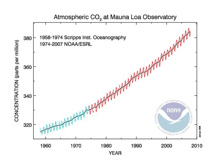
This record illustrates an increase in the average (the little wiggles are seasonal variations) pCO2 (partial pressure of carbon dioxide in the atmosphere) of about 19 percent over the past half century. Of course, it is this increase that global warming has been attributed to, but there is another issue. Even if we could mitigate global warming by some engineering miracle (mirrors in space, etc.), the increase in pCO2 would probably ultimately get the corals. Why? Because the increase in pCO2 and its penetration into the ocean surface lowers the pH of the ocean, decreasing the carbonate ison concentration and, ultimately, decreasing saturation with respect to aragonite. Figure 7-3 shows how this works with some simple calculations by doubling pCO2.

Note that through reactions shown (carbonic acid equilibria in seawater) doubling pCO2 from its pre-industrial level (280 ppm) to 560 ppm substantially decreases pH (by 0.24 units) and carbonate ion concentration (by about 34 %); of course, we have not gotten to that point--yet! Note, however, that atmospheric CO2 derived from fossil fuels (how do we know this?) has mixed down into surface waters and penetrated deeper into the ocean (remember the deep circulation?) in some regions as shown in Figure 7-4. This is causing a decrease in pH.
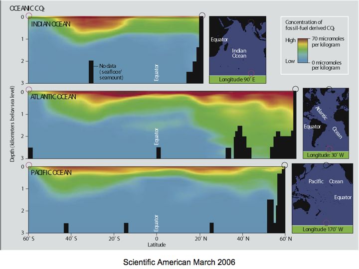
Chris Langdon (Lamont Doherty Earth Observatory, Columbia University) grew corals artificially in Biosphere 2, Arizona and subjected them to different pCO2 levels. He found that their growth rate decreased with increasing pCO2 as shown in Figure 7-5.
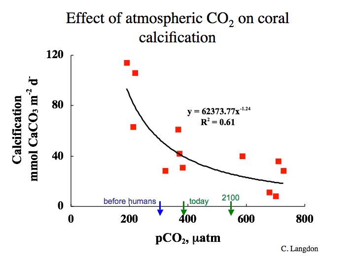
Ocean Acidification and Coral Reefs
Let's take some time to reflect on what we've just covered on coral reefs! Here you may want to think about how you would help students understand the principles underlying the conclusion that corals are in trouble because of increasing carbon dioxide concentration in the atmosphere. The underlying chemical equilibria are complex, but must be understood at some level in order to be able to analyze and accept the scientific conclusions. Who or what are we if we take others word alone for such things, or dismiss it because we cannot understand it?
We want you to read and study the recent work by reporter Craig Welsh and the following two accessible and (reasonably) short semi-technical papers about the problem of "ocean acidification" and its consequences:
The Seattle Times [133] (don't forget to click on some of the "Sea Change Stories" in the right margin. They are well done and visually stunning!)
Kleypas and Langdon (2003) Conference Proceedings Summary [134]
Doney (2006) Scientific American [135]
These should give you a feeling for the background, chemical principles and uncertainties in drawing conclusions about the developing trend in ocean acidification.
Activity 3: Simplifying the Problem
For this activity, let's use a common classroom technique to explain the complex issue of ocean acidification. Activity 3 should be posted to the discussion board for Lesson 7
- Become an organism (your choice...urchin, starfish, seagull, something else?) that is affected by the issue of ocean acidification (either directly or indirectly). Write a 750 word (or so...) letter to humans to fix the problem. Clearly some of these concepts are complex, so do your best to simplify them without losing the science. Make it fun and stay in character. Your letter should include and understanding of:
- human/atmospheric contributions to ocean acidification
- scientific process of acidification
- organisms affected (with statistics/data)
- potential consequences
- possible solutions
- Comment on 2-3 of your colleagues' posts with a twist! When you comment, stay in character as the organism you chose for part "A" (please remind us who/what you are when you comment so we have context for your comments). Ask a question, argue a point, elaborate on some evidence, etc.
See the grading rubric [12] for specifics on how this assignment will be graded.
Additional Resources
- Gulf of Mexico Dead Zone news and information at Louisiana Universities Marine Consortium
- Harmful Algal Blooms resources at Woods Hole Oceanographic Institution
- Scientific resources for ocean acidification at the ocean-acidification network
- Coral reef health and biodiversity research at NASA (remote sensing)
- International Reef Check program
Tell us about it!
Have another reading or Web site on these topics that you have found useful? (Or, if you were offended by Mike's edgy, profane pun on the previous page) Share it in the Comment area below!
Summary & Final Tasks
What can we say? If you are here, you must think that you are done. You are, after you follow the advice below. You are about 7/9ths through this course. Hope you are having some fun. Tired of doom and gloom? Wait until Lesson 8! Hope you don't like seafood!
Reminder - Complete all of the lesson tasks!
You have finished Lesson 7. Double-check the list of requirements on the Lesson 7 Overview page to make sure you have completed all of the activities listed there before beginning the next lesson.
Once you've completed all lesson tasks, make sure you enter the "Teaching and Learning" discussion in Canvas and tell us how you would teach a topic from this lesson in your own classroom
Tell us about it!
If you have anything you'd like to comment on, or add to, the lesson materials, feel free to post your thoughts below. For example, what did you have the most trouble with in this lesson? Was there anything useful here that you'd like to try in your own classroom? Is climate change a topic you and your students are interested in? Do your students have much interest in or opinions about the politics/science of global climate change?
Lesson 8
Lesson 8 Introduction
The Secret Lives of Fishes and the Great Meal Deal
About Lesson 8
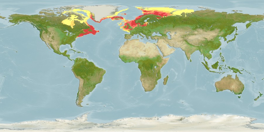
In this lesson, we will review life in the ocean and focus in particular on aquaculture and the problems of overfishing.
By the end of this lesson you should be able to describe the main elements of the food chain in the ocean, including the importance of photosynthesis and phytoplankton. You should also be able to summarize current practices and trends in aquaculture and the main threats to natural marine fisheries.
What will we learn in Lesson 8?
By the end of Lesson 8, you should be able to:
- Describe the food chain in the ocean
- Explain why photosynthesis is important to life in the ocean
- Explain the importance of nutrients in the ocean
- Explain the energy cycle of the ocean, with specific reference to nutrient cycling
- Describe the spatial distribution of life in the ocean and give reasons why fish biomass is concentrated where it is
- Describe aquaculture including where it is practiced, recent trends in farmed fish, and salient pros and cons of aquaculture
- Describe the state of ocean fisheries and summarize the main threats to fish populations in the ocean
- Explain what is being done to save marine fisheries and the nature of the problems with designing and enforcing fishing regulations in the open ocean.
- Use on-line resources to construct maps of fisheries
What is due for Lesson 8?
The chart below provides an overview of the requirements for Lesson 8. For assignment details, refer to the lesson page noted. See the Course Schedule (located in the Resources menu) for assignment due dates.
| REQUIREMENT | LOCATION | SUBMITTED FOR GRADING? |
|---|---|---|
| Activity 1: Fisheries | page 3 | Yes |
| Activity 2: Empty Oceans | page 4 | Yes |
Questions?
If you have any questions, please post them to our Questions? discussion forum (not e-mail), located under the Communicate tab in Canvas. I will check that discussion forum daily to respond. While you are there, feel free to post your own responses if you, too, are able to help out a classmate.
The Secret Lives of Fishes and the Great Meal Deal
Life in the ocean: it's all about finding a good lunch spot
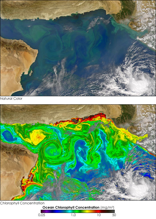
Reading
- Please review these slides [138].
The following are key points in the ppt slides
- Importance of simple photosynthetic organisms (phytoplankton) to the food chain in the oceans.
- Importance of nutrients and sunlight to phytoplankton growth
- Fish live close to their food supply, and/or, they travel huge distances for special feeding events
- How are nutrients supplied to the photic zone?
- What happens to all of the food (organic matter, carbon) produced in the photic zone? Is it buried as sediment at the bottom of the ocean?
- Energy cycle of the ocean, composting, role of bacteria
- Why are deep waters important for phytoplankton growth?
- Good background reading for phytoplankton importance [137]
Aquaculture and the future of marine fisheries
Aquaculture
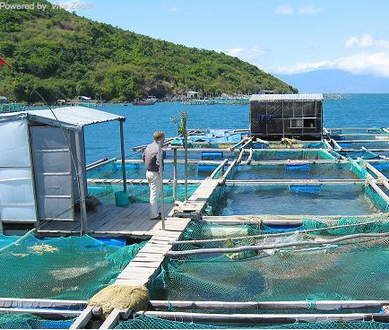
Required Reading
- Aquaculture: Should it be located offshore? (pdf file) [140]
- Lawmakers, Enviros Maneuver in Last-Gasp Bid to Block Deepwater Aquaculture, NY Times, 3 Aug 2009 [141]
Background information. FYI
- Organic Aquaculture, is it possible? [142] Recent work draws wide-range criticism
- NOAA's Aquaculture program [143] A vision for the future?
Fisheries and Issues of Global Catch; Activity 1
The Ocean is vast, but its resources are finite
Empty Oceans Empty Nets (this is an excellent movie on the subject) [144]
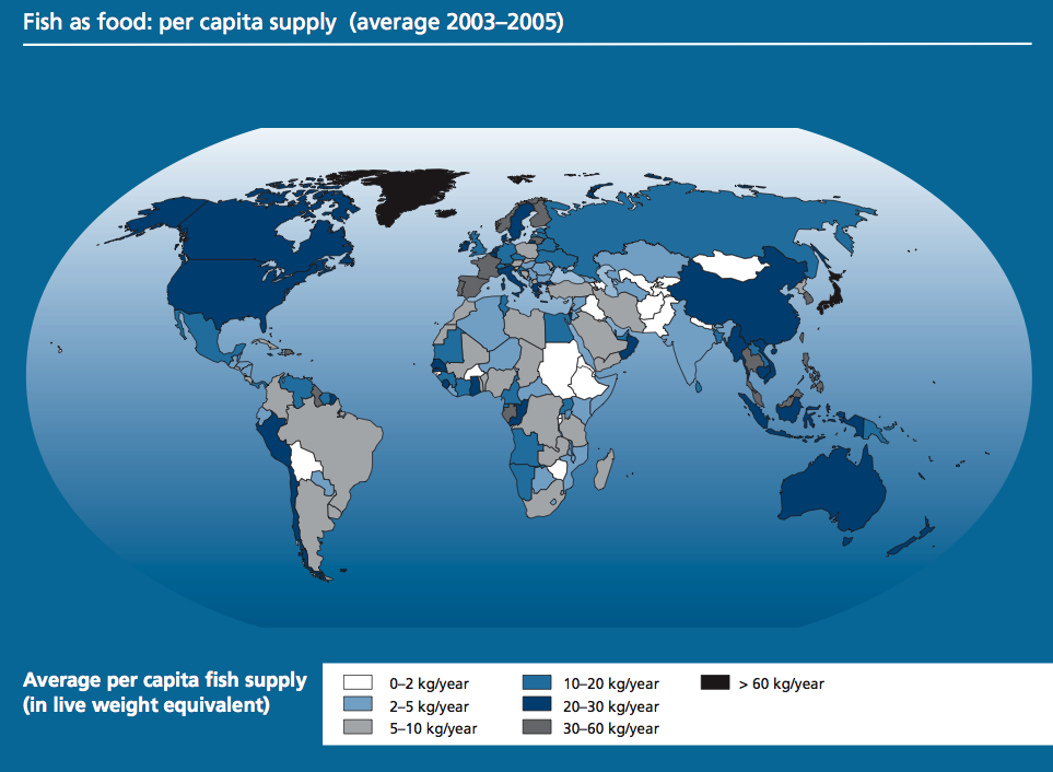
Reading
- THE STATE OF WORLD FISHERIES AND AQUACULTURE [146] The definitive and most recent study of world fisheries written by the Food and Agriculture Organization of the United Nations (FAO)
Activity 1: Fisheries
- Scan/read the document from FAO and pick 4 or 5 of the most compelling plots and/or data sets. Give details about where to find them (so that others can find them in the document) and summarize, in a few sentences for each, why you chose them. Use the Canvas Discussion forum.
- Respond to a few of the blogs written by other students
Grading criteria
See the grading rubric [12] for specifics on how this assignment will be graded.
Empty Oceans Empty Nets; Activity 2
The Ocean is vast, but its resources are finite
Empty Oceans Empty Nets
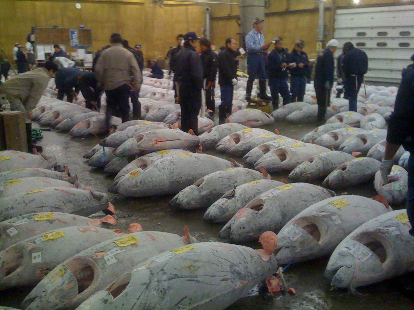
Visit WPSU's Marine Fisheries & Aquaculture Series [144] and read about the problems with overfishing. This PBS documentary is a must see. You may be able to get it from your local library. If not you could buy it (it's a great thing to show to your classes). I've also collected a few youtube links with interesting shorts on related topics.
Reading
Click on the links below. I have provided some guidance about what to focus on, but these are excellent resources, so you are encouraged to read beyond my suggestions.
- Oceans of Nothing [147] A study says overfishing will soon destroy the seafood supply. Read this first and then look at the slides by Boris Worm (next link below)
- How loss of ocean species threatens human well-being [148] What happened to all the big fish? Slides by Boris Worm
- Empty nets and empty stomachs [149] Clips from a television documentary about local problems with global fleets
- Humorous commercial about a big problem involving small fish [150] You should also check out OceanLegacy.org
- Investing in our future [151] Check out this web site for recent information on government involvement in the problem of overfishing
- Greenpeace, Overfishing [152] Many marine ecologists think that the biggest single threat to marine ecosystems today is overfishing
Activity 2: Empty Oceans
- Create a 400-500 word "script" for a compelling commercial that discusses the issues of overfishing. Think Political Ad (or don't...). Feel free to set the scene for us and then provide some dialog. Compel us to act! Post your script in the Canvas discussion. Emphasize one or more of the following: data documenting the problems, local vs. national and international solutions, creative solutions.
- Respond to several of the scripts written by other students
Grading criteria
See the grading rubric [12] for specifics on how this assignment will be graded.
Almost there!
- Just the capstone left!
- Give yourself a huge pat on the back for a job well done!
- If you haven't already done so, please provide feedback on the course using the University’s online Student Educational Experience Questionnaire (SEEQ) system, which you can find in Canvas.
Lesson 9
Activity: Capstone Project
In this activity, you will design a lesson for an audience of your choosing based on one of the topics we covered in this course.
Directions:
1. By August 3 - Figure out approximately what you want to teach and email me a brief description of your plan and your audience. For example, you could just say "I'm going to design a lesson where high school students investigate ocean surface currents" or something like that.
2. By August 12 - Write up your lesson plan. Your lesson plan should include the following:
- A brief overview of what will be taught and why
- A set of learning objectives (What will your students know or be able to do at the end of your lesson?)
- A description of your plan (What will the students do?)
- List of necessary materials
- A list of deliverables (What will the students turn in? How will you know if they learned what you wanted them to learn?)
- An evaluation rubric (so that another teacher could assess the students in the manner that you intended)
- Save an electronic version of your activity as either a Microsoft Word or PDF file in the following format: L9_capstone_AccessAccountID_LastName.doc (or .pdf).
Submitting your work
Upload your capstone project file to the Lesson 9 dropbox in Canvas.
Note on Grading:
I am interested in the scientific accuracy of the topic you choose to teach. I am not going to base my grade on whether you have constructed a lesson plan in some special way (as long as all the components listed above are there). My assumption is that for those of you who are teachers, you don't need me to tell you how to write a lesson plan because you already know. For those of you who are not teachers, I am not the one who is going to instruct you on correct lesson plan-making. However, I am a scientist and an educator, so if facts are not right, or could use clarification, I can assist with that.
Grading rubric
An "A" capstone project is complete, clear, and organized. It contains all the components listed above. The science is accurate. I can follow your instructions and get the results you expected me to get. The questions you made up are well-designed and would elicit the appropriate amount of thinking and interpretation on the part of the intended audience. Your project shows independent thinking.
A "B" capstone project is like that of an "A" project, except that its directions may not be clear enough that I can follow them without having to guess a little bit about your exact intentions. A "B" write-up is complete and contains all the components listed above.
A "C" capstone project may have clarity problems, leading me to have to guess how to follow your instructions. A "C" write-up may also be incomplete with some of the assignment components missing. The science may not be accurate.
A "D" capstone project has such badly written directions that I can't even begin to guess how to follow your instructions. A "D" write-up may be significantly incomplete and it may contain gross factual errors.