Lesson 2
Lesson 2 Introduction
Living on an Island: Origin of Ocean Basins and Sea Floor Morphology
About Lesson 2
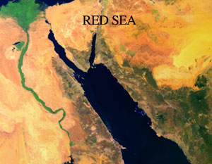
In one sense or another, we are all Living on an Island. The continents are buoyant rock masses that are floating in the Earth’s mantle-asthenosphere and surrounded by water at the surface. Earth’s surface is in constant motion and the ocean basins are continually evolving. The image of the Red Sea on this page is an example of some of the most recent change—an ocean basin is forming! We’re going to spend Lesson 2 exploring the Origin of the Ocean Basins and learning about how Sea Floor Morphology relates to the processes that have shaped the current ocean geometry. As I suspect you know, this all starts with Plate Tectonics and Sea Floor Spreading.
By the end of this lesson you should have a deeper understanding of: plate geometry and kinematics, the role of earthquakes, hot spots and how they relate to volcanic edifices, and continental margins. One of the things to think about this week is how you might develop a teaching module on Plate Tectonics.
What will we learn in Lesson 2?
By the end of Lesson 2, you should be able to:
- Explain the basic tenets of plate tectonics including relative and absolute plate motion.
- Use spherical trigonometry to calculate linear and angular distances on Earth’s surface. Employ this knowledge to work with plate motion vectors
- Use on-line resources to calculate rates of plate tectonic motion.
- Explain hot spots at a basic and sophisticated level, including how they can be used to determine relative plate motion, past theories of their origin, the concept of “Mantle wind,” and current ideas about their origin.
- Describe the Wilson Cycle and related concepts of Sea Floor Spreading.
- Discuss Earth’s internal structure, including the relationship and distinctions between chemical classifications (Crust, Mantle, etc.) and rheologic classifications (Lithosphere, Asthenosphere…).
- Readily point out examples of the three basic plate boundaries and their tectonic, seismic and volcanic manifestations at Earth’s surface.
- Use on-line resources to construct maps of the ocean floor
What is due for Lesson 2?
The chart below provides an overview of the requirements for Lesson 2. For assignment details, refer to the lesson page noted. Due dates are listed in this table and in Canvas.
| REQUIREMENT | LOCATION | SUBMITTED FOR GRADING? |
|---|---|---|
| Activity 1: In five easy parts... | see "activity 1" in lesson 2 menu | Yes - You should put a file with your answers in the Canvas dropbox, due June 16th |
| Activity 2: Make map images and comment in a discussion forum. | see "activity 2" in lesson 2 menu | Yes- You should put a file with your answers and comments in the Canvas dropbox |
| Activity 3: Hotspots, background reading and discussion | see "activity 3" in lesson 2 menu | Yes- Discussion responses will be graded. |
Questions?
If you have any questions, please post them to our Questions? discussion forum (not e-mail), located in the Discussions menu in Canvas. I will check that discussion forum daily to respond. While you are there, feel free to post your own responses if you, too, are able to help out a classmate.
Overview
We need a basic understanding of plate tectonics in order to appreciate how the ocean basins have evolved over geologic time and how they will evolve in the future. I suspect that many, if not all of you, are experts on plate tectonics, and the M. Ed. program at Penn State has a course devoted to the Solid Earth (Earth 520), so we won’t cover things in an exhaustive/comprehensive fashion. Instead, we’ll pick a few representative activities that will highlight the connections we need for Oceanography and help you to see what additional background would be useful for you.
A brief background on Plate Tectonics and Continental Drift
The notion that plates move has been around since at least early 1900's. Alfred Wegener, a German Meteorologist, proposed the theory of Continental Drift. He used a variety of observations to argue that the continents had moved and broken apart –including the shapes of coast lines, palaeontological and botanical data, and geological data. But he lacked a credible theory for motion. Physicists of his day dismissed the notion that the continents could move because they thought Earth’s interior was solid and rigid. Nevertheless, various people worked on the theory and proposed modifications. One such was Alex Du Toit, a south American geologist who collected geologic observations from both sides of the south Atlantic and published them in the 1930’s. A number of discoveries in the 1950’s and early 1960’s, including age dating of rocks and magnetic signatures in rocks, led first to the theory of ‘sea floor spreading’ and then to the theory of plate tectonics. A naval captain, Harry Hess, proposed sea floor spreading on the basis of bathymetric profiles he made in the pacific. His data showed that ocean depth increased systematically and symmetrically from a long, axial ridge. Hess’ data were combined with other key observations (including magnetic stripes, heat flow, seismicity along plate boundaries) and ideas (mantle convection) to form the theory of plate tectonics.
Tenets of the theory:
- Plates are rigid
- Earth is a perfect sphere (and points on it can be specified with a radius vector)
- Plates move tangential to the radius vector.
- Material is created and destroyed at spreading ridges and subduction zones, but not at transform boundaries.
- Transform faults form small circles to poles of rotation.
Three important issues for plate tectonics
Issue #1: Earth’s Internal Structure
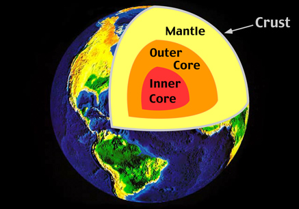
The Earth’s internal structure is made up of three layers called the crust, mantle, and core. The crust is the outermost layers made up of solid rocks mostly silicon and aluminum. The mantle is the layer beneath the crust and made up of mostly silicon and magnesium. The mantle has two layers called the upper mantle and the lower mantle, collectively called the lithosphere. The oceanic and continental plates are in the mantle. The core is the innermost layer of the Earth and is made of solid iron and nickel. The outer core is a liquid layer beneath the mantle and the inner core is the center of the Earth.
Note that there is a distinction between features defined by chemical composition (Crust, Mantle, Core, as shown in the sketch) and those defined by rheology (Lithosphere, Asthenosphere, Mesosphere --not shown here).
Check this out!
A few cool facts:
- The density contrast between the Lithosphere (roughly 2.5 to 3 gm/cc) and the Atmosphere above it (roughly 0) is not nearly as big as that between the Outer Core (roughly 11 gm/cc) and the base of the Mantle (roughly 6 gm/cc).
- Good place to learn more about Earth Structure. [3]
- Better place to learn more about Earth Structure. [4]
- Look at how thin the Crust is! Challenge: Find a better Earth analog than a Major League Baseball (see Activity 1)
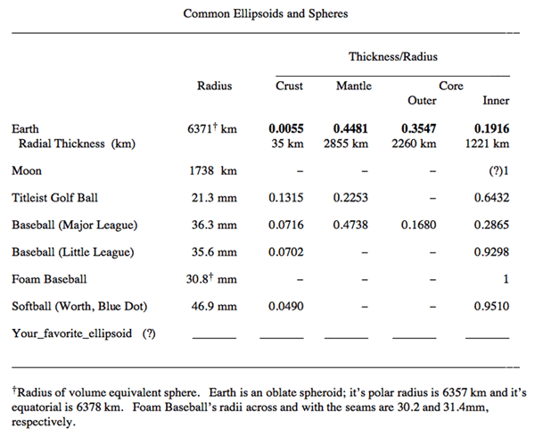
Click for text description of the common ellipsoids and spheres image
Text Description of Common Ellipsoids and Spheres Table
Common Ellipsoids and Spheres Ellipsoid/Sphere Radius Thickness/ Radius: Crust Thickness/ Radius: Mantle Thickness/ Radius: Outer Core Thickness/ Radius: Inner Core Earth
Radial Thickness (km)6371†km 0.0055
35 km0.4481
2855 km0.3547
2260 km0.1916
1221 kmMoon 1738 km - - - (?)1 Titleist Golf Ball 21.3 mm 0.1315 0.2253 - 0.6432 Baseball (Major League) 36.3 mm 0.0716 0.4738 0.1680 0.2865 Baseball (Little League) 35.6 mm 0.0702 - - 0.9298 Foam Baseball 30.8† mm -- - - 1 Softball (Worth, Blue Dot) 46.9 mm 0.0490 - - 0.9510 Your_favorite_ellipsoid (?) _______ _______ _______ _______ _______ †Radius of volume equivalent sphere. Earth is an oblate spheroid; it's polar radius is 6357 km and it's equatorial is 6378 km. Foam Baseball's radii across and with the seams are 30.2 and 31.4 mm, respectively.
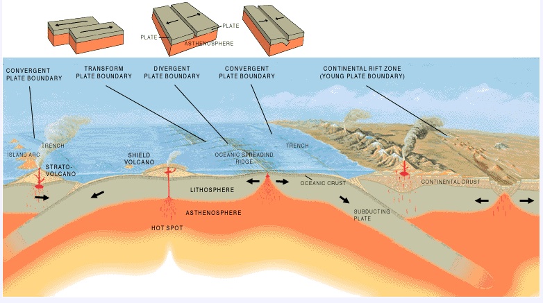
Issue #2: Plate Boundaries
There are three types of plate boundaries:
- Divergent,
- Convergent, and
- Transform.
In the parlance of structural geology: Divergent Boundaries correspond to normal faults, Convergent Boundaries correspond to thrust (or reverse) faults, and Transform Boundaries correspond to strike slip faults .
Want to learn more?
If you’d like more background on Faulting, see the page on "Faults" [6] from Prof. Eliza Richardson’s course, EARTH 520: Plate Tectonics and People.
Issue #3: Earth is an oblate sphere, which means it is elliptical!
Okay! The main thing is that it's roughly spherical (NOT flat!). The average radius of Earth is 6,371 km and the radius is nearly 22 km larger at the equator than at the poles (it's an ellipsoid, rather than a perfect sphere!). The lithospheric plates move on the outer surface of a sphere, so it's convenient to describe plate motion in terms of a rotation about a point on Earth's surface (or a rotation vector that hypothetically extends from Earth's center to the surface point). This point is called the pole of rotation, or just the rotation pole.
Let's start with a useful formula for the radius:
Earth is not a perfect sphere: its ellipticity can be written:
where Re is the equatorial radius=6378.14 km, and Rp is polar radius=6356.75 km. To first order, the variation in radius with latitude, , can be written:
Want to learn more?
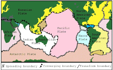
Read about changes in Earth’s shape due to climate events in the following NASA article: "Some changes in Earth's Shape Are Due to Changes in Climate [7]."Map view symbols for plate boundaries
.jpg)
Want to learn more?
Want more background or do you need more help with plate boundaries and plate names? Take a look at This PBS Learning Site [8]
Try this!
Can you identify the type of faulting occurring at each plate boundary in the map below? What type of faulting is depicted between the Nazca and South American plates?
Plate Motion and Activity 1
Let's do something with Plate Tectonics and ask how fast plates move relative to one another? The answer can be found by using plate rotation vectors. Stick with me for a minute or two. This looks more complicated at first blush than it really is. For our purposes, we just need the ability to plug numbers into an equation --so we need to follow the parameter definitions and the equation.
Want to learn more?
See "Simple Euler Poles [11]."
The motion of a point on one tectonic plate relative to another plate can be described by the relative velocity vector v. The velocity v has magnitude and direction and is given by the cross product of the angular velocity vector ω and the plate rotation vector r . The equation looks like this, where the "x" means cross-product. The reason we can't just use distance=rate*time is because we are describing the motion on the surface of a sphere as opposed to making the assumption that it's all flat and distances are simply linear.
v = ω x r
For example, according to one of the accepted models for plate motion (NUVEL 1), the velocity of the North American Plate relative to the Pacific Plate is given by the rotation pole at: 48.7° N 78.2° W and angular velocity 7.8x10⁻⁷ degrees/year (that is: 0.00000078 deg/year.) Therefore, a point on the Pacific plate near Parkfield California, which is at 35.9° N 120.5° W, is moving at 47.6 mm/yr relative to the rest of North America. How long will it take for this point to reach the present location of San Francisco?
How does this calculation work? Download this pdf file for the details [12]. That file contains some useful background. The last page is the example above.
NOTE: Parkfield CA is the site of a National Science Foundation project called EarthScope [13] that has drilled into the San Andreas Fault. See SAFOD Observatory [14] for more details on the drilling project.
One of the first sketches to show tectonic plates
Note the three types of plate boundaries (compare to the figure on the previous page) and the definitions of lithosphere, asthenosphere, and mesosphere. Lithosphere means the rigid part and thus the bottom of it is defined by an isotherm (do you know why?). The base of the lithosphere is typically taken as 1300° C. Note that the plate thickens as it moves away from a divergent spreading center. Mid-ocean ridge systems are hot (they are volcanoes!) and thus ridges are relatively buoyant, which means that they have relatively higher elevation than regions around them. Ocean depth increases systematically with distance away from mid-ocean ridge systems. We'll look at this more closely in Activity 3.
Note in the sketch below that the Earth and its plates are portrayed as a block instead of a sphere. If you think spherical geometry is difficult to work with, you are right. It's hard to visualize in your head and not so easy to sketch, either.
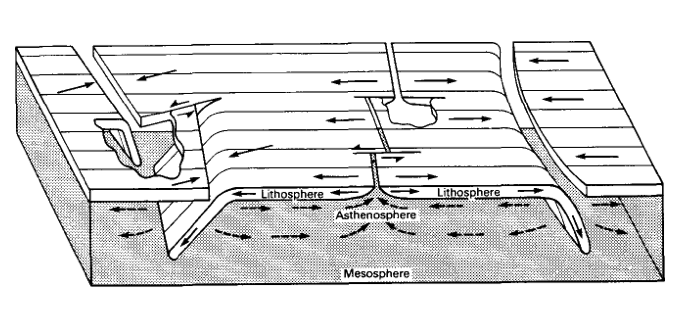
Plate motion vectors
You can always use vector algebra to calculate linear velocity v from the position vector r and the angular velocity vector ω, but there's an easier way to get the magnitude of the velocity by using the solid angle between the pole of rotation and the location of interest (see below). The solid angle can be obtained using spherical trigonometry:
cos a = cos b cos c + sin b sin c cos A
where a is the solid angle of interest, b is the co-latitude of the location on Earth's surface, c is the co-latitude of the plate rotation pole and A is the surface angle between the pole and the location (that is: A is the difference between the longitude of the pole and the longitude of the location).
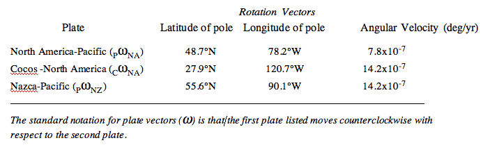
Plate Motion Vectors
Credit:Prissy.US
Click for text description of the plate motion vectors table.
Text Description of Rotation Vectors Table
| Plate | Latitude of pole | Longitude of pole | Angular Velocity (deg/yr) |
|---|---|---|---|
| North America-Pacific (PNA) | 48.7°N | 78.2°W | 7.8x10⁻⁷ |
| Cocos-North America (CNA) | 27.9°N | 120.7°W | 14.2x10⁻⁷ |
| Nazca-Pacific (PNZ) | 55.6°N | 90.1°W | 14.2x10⁻⁷ |
The standard notation for plate vectors () is that/ the first plate listed moves counterclockwise with respect to the second plate.
Some background on Spherical Trigonometry
To work with plate motion vectors, and to calculate the linear velocity of points on Earth's surface, we need to know the distances between various points on the globe. A useful analogy is that of linear and angular velocities associated with Earth's daily rotation. That is, the angular velocity is the same everywhere on Earth. All points rotate through 360° (2 pi radians) in 24 hours. But the linear velocity, on Earth's surface, depends on where you are relative to the rotation axis. If you're at the North Pole, then you cover only a small distance, whereas if you're at the equator, then you cover a distance equal to Earth's full circumference in 24 hours (2 pi R). As Earth rotates each day, the linear velocity of points at the Equator is much larger than points near the poles. The same type of thing happens with plate motions. Points that are close to the pole of rotation move with lower linear velocity than points that are farther from the pole. So, we need to calculate the distance between each point and the pole. These next two figures will help show how this works. Remember, for our purposes, we just need to be able to plug numbers into an equation, so we need to follow the parameter definitions and the equation.
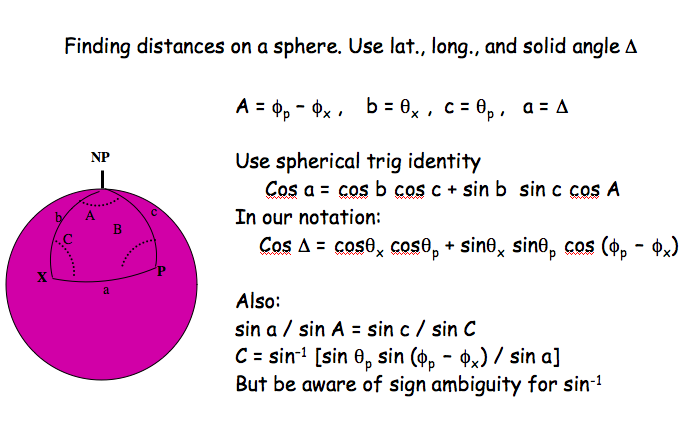
Click for text description of the spherical trigonometry image.
Use spherical trig identity
In our notation:
Also:
But be aware of sign ambiguity for sin-1
In the diagram above, upper case letters refer to surface angles and lower case letters refer to solid angles, measured between lines that extend from the Earth's center to the surface. For a point X at, say, latitude 20° N, the angle b is 70°, because b is measured from the north pole along a line of longitude. In the calculation, it's standard to use the 'co-latitude' b and c. Note that it's easy to get b and c, based on their latitudes. But the same is not true for the solid angle a. That's why we need spherical trig. Surface angles are perhaps more familiar. They are obtained from latitude and are therefore nothing more than a larger-scale version of the angle between the first-base line and the third-base line on a baseball diamond.
Here's an example that will help to fix ideas. Do you follow? If not, please post a question on Canvas.
Click for text description of the spherical trigonometry example image.
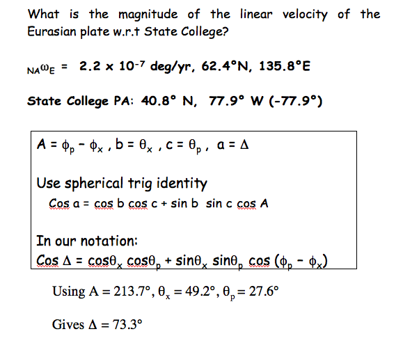
What is the magnitude of the linear velocity of the Eurasian plate w.r.t State College?
State College PA: 40.8°N, 77.9°W (-77.9°)
Use spherical trig identity
In our notation:
Check: Can you verify 73.3 deg. for this example? If not, make sure you're using co-latitude and that your answer is in degrees. Still having trouble? Then have a look at this [15].
Magnitude of linear plate velocity
Once you have the angular distance between the points (Δ), you can get the linear velocity using v = ω R sin Δ. See the last page of this pdf file for a worked example [16].
Activity 1
NOTE: For this assignment, you will need to record your work on a word processing document. Your work is best submitted in Word (.doc), or PDF (.pdf) format so I can open it.
Directions
- Find an analog for Earth's internal structure and measure the relative thicknesses of the layers. Here is an image that goes along with mine (a major league baseball), see details of my numbers on the previous page:
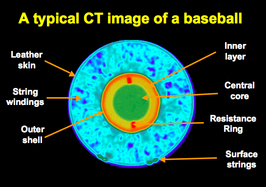 A typical CT image of a baseball
(Are you a fan? Here's a short set of ppt images showing how baseballs have changed over the years.) [17] - Using the formula given on the previous page, calculate Earth's radius at your location. Here's how: look up the latitude of where you are, and then plug-and-chug. This is the relevant equation, so you don't have to go back and find it again: in which Re is the equatorial radius=6378.14 km and lambda is your latitude, and f is the Earth's ellipticity: can be written: where Rp is polar radius=6356.75 km.
- Now, we're ready for a real problem. Calculate the rate of motion between the Pacific Plate and the North American Plate at Hollywood, CA. (I worked the example of the Golden Gate Bridge for you.) I expect that you will show enough of your work so that I can follow how you did the calculation. At the least, you should list all of the parameters and factors used in your calculation. Even better is to paste in your calculation from Google or elsewhere, as in this example: http://www3.geosc.psu.edu/~cjm38/540/sphericaltrigExample.html [15]
- 37.8 N 122.5 W (the golden gate bridge) [18]
- 34.1° N 118.3° W (Hollywood, CA)
- Check both sites using the plate motion calculator [19] at the UNAVCO Web site.
NOTE: To start, you can enter just the latitude and longitude of the point of interest and hit submit. You'll get an answer, with default parameters. Hmm, does it work to just copy/paste in the numbers above? What happens if you write 122.5 W vs. -122.5? Can you include the ° symbols?
For our example problem, you should set the Reference to "PA Pacific" when doing the Golden Gate case, and "North America" when doing Hollywood (what happens if you choose Pacific for the Hollywood case?). You can also try NNR (no net rotation). Play around with this a bit. It's useful!
Under "Model" select "All of the above" so that you can see the range of predictions. Tell me your thoughts on why there are differences in the predicted rates of motions. What happens if you use a different frame of reference?
- Go to the UNAVCO Web site [20] and determine a plate motion rate using their GPS data for the Mission Viejo, CA station. Do two things: calculate a linear velocity like we did in #3, having read the latitude and longitude of this station on its web page. Then use the plots of GPS data to calculate an approximate linear velocity using the Pythagorean theorem, as in north2 + east2 = total2. The link will take you to the UNAVCO page for Mission Viejo, CA (SBCC). (Note: The folks at UNAVCO sometimes modify their web page. If you have trouble finding the data, use this file [21]).
- You have now calculated plate motion at three different places on the North American plate with respect to the Pacific plate using spherical trigonometry. You have compared those calculations to two other methods (using UNAVCO's calculator and using properties of right triangles). Discuss in a few sentences the similarities/differences between the different calculated values and whether you think the differences are due to rounding errors, geographic location, other assumptions, and so forth. If you wanted to make an estimate the quickest way, which method would you use? If you wanted the most accuracy, which would you choose?
- Save your document as either a Microsoft Word or PDF file in the following format:
L2_activity1_AccessAccountID_LastName.doc (or .pdf).
For example, student Elvis Aaron Presley's file would be named "L2_activity1_eap1_presley.pdf"—this naming convention is important, as it will help me make sure I match each submission up with the right student!
Submitting your work
Upload your paper to the "Lesson 2 - Activity 1" dropbox in Canvas by the due date indicated on our Course Schedule.
Grading criteria
See the grading rubric [22] for specifics on how this assignment will be graded.
Activity 2; Motion Under the Ocean, Hot Spots
Activity 2
NOTE: For this assignment, you will need to record your work on a word processing document. Please submitted in Pages, Word (.doc), or PDF (.pdf) format so I can open it. Also, this doesn't have to be long. What I want is the figures I mention and some text to go with them that describes what you did and what you concluded. If we were in a classroom together I imagine this would be like an in-class or in-lab exercise, meaning I'm expecting you could do a reasonable job in an hour or two, depending on your reading speed and any prior experience with Google Earth.
Directions
- First, read this short paper. It's important background for mid-ocean ridges and the bathymetry around them:
- Macdonald, K.C. and P.J. Fox, The mid-ocean ridge [23], Scientific American 262:72-79, 1990.
- Download Google Earth [24] and spend enough time with it to make an image of the ocean floor. In particular, look at the bathymetry around a mid-ocean ridge spreading center. Paste your image into a word processing document as noted above. Note that you should look at parts 3 and 4 before you complete this.
- In your document, comment briefly on how seafloor depth and morphology varies with increasing distance from a mid-ocean ridge spreading center. For example, I'm hoping you'll produce an image in part 1 that will tie-in with the article noted above. (Can you find some of the features they discuss? If you can, describe where they are. If not, or if you aren't sure, think about any differences in our ability to image the sea floor now versus when the paper in part 1 was written.) Think big, don't limit yourself to a few km from the spreading ridge; consider seafloor morphology at the scale of an entire ocean basin, like this example image of the Ocean Basin [25].
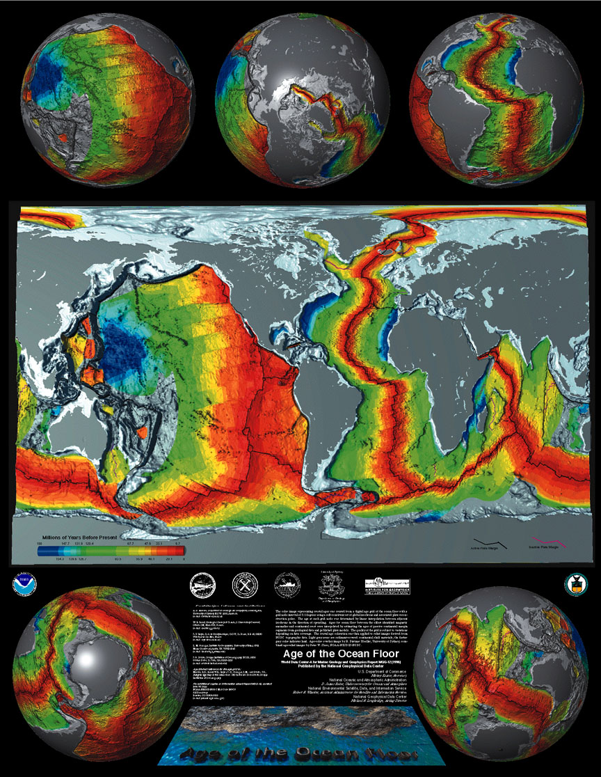
- Look at the Crustal Age [26] Poster [26] from NOAA. Download the image, take a screen shot, or use another approach to make a map of the ocean floor showing seafloor age. Add one or two other features to your map, and describe in a few sentences whether you could use a Web site like this in one of your classes. Paste your images into the word processing doc along with your comments.
- Save your document as either a text, Pages, Microsoft Word, or PDF file in the following format:
L2_activity2_AccessAccountID_LastName.doc (or .pdf).
For example, student Elvis Aaron Presley's file would be named "L2_activity2_eap1_presley.doc"—this naming convention is important, as it will help me make sure I match each submission up with the right student!
Submitting your work
Upload your document to the "Lesson 2 - Activity 2" dropbox in Canvas (see Dropboxes folder under the Assignments tab) by the due date indicated on our Course Schedule.
Grading criteria
See the grading rubric [22] for specifics on how this assignment will be graded.
Activity 3: Discussion about recent hot spot research papers
Now that we are experts on Plate Motions, let's think about how Volcanic Island Chains work and how they can help to understand plate tectonics and ocean process.
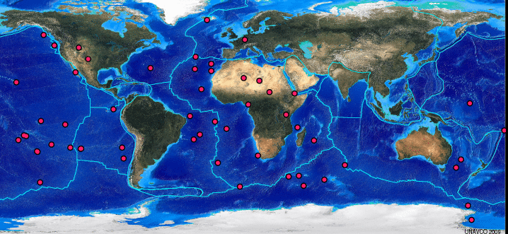
The dots on the map below show locations of major Hotspots on Earth's surface.
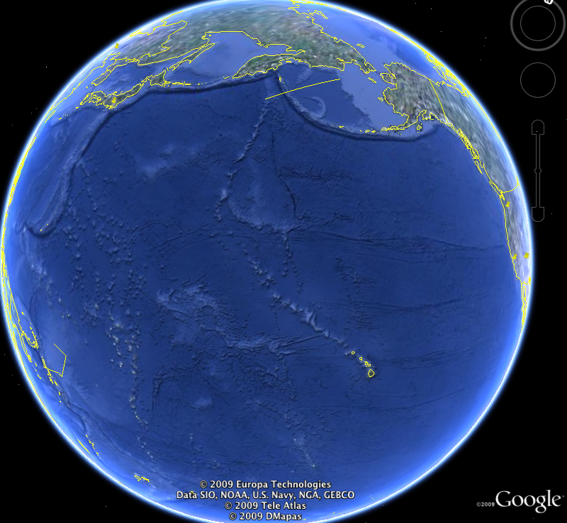
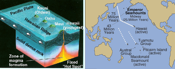
I made the image below with Google Earth. It shows the Hawaiian Island Chain and the Emperor Seamount Chain. Follow the linear track to the northwest from the Hawaiian islands (yellow lines show island coastlines). The features that are not outlined in yellow are below sealevel; they're called seamounts. The Hawaiian chain connects to the Emperor Seamount Chain, which has a more northerly trend. The seamounts are extinct volcanoes. Each one of them was once located over the Hawaiian Hotspot.
Want to learn more?
- More information about hotspots, see "'Hotspots': Mantle thermal plumes. [28]"
Hotspots and Ocean Floor Morphology
Hotspot tracks on the ocean floor were one of the first smoking guns for the theory of plate tectonics, and they were also one of the conundrums. Early evidence showed that hotspots were more or less fixed in space; they did not seem to move relative to one another. This led to the idea that they originated at great depth. But how could a narrow plume of heat, or low viscosity material, rise through the convecting mantle without being offset? Early researchers pointed to the analogy of smoke rising through the atmosphere: on a windy day, the smoke plume was offset, and when the wind changed direction, so did the plume.
The images below shows a basic idea of how hotspots and linear island chains work.
Activity 3
Directions
- Refer to these short papers:
- Post your responses to the following questions in the discussion area on Canvas for Lesson 2 Activity 3.
- Why do hotspots form distinct volcanic islands, rather than a continuous linear axis?
- What major change occurred recently in our thinking about Hotspots, and what were the data that led people to rethink the way hotspots work?
- Many textbooks say that the change in trend of the Hawaiian Islands and the Emperor Seamounts represented a major shift in the direction of the Pacific plate motion ~ 43 Ma. Is that still thought to be true?
- Read the postings made by other EARTH 540 students.
- Respond to at least two other postings, per question, by asking for clarification, asking a follow-up question, expanding on what has already been said, etc. You should have at least six responses to other postings.
Submitting your work
- I have begun this discussion activity by posting each of the 3 questions to the discussion on Canvas. Please click on the "reply" link that follows each question in order to post your response. To respond to another student's posting, use the "reply" link that follows their posting.
Grading criteria
You will be graded on the quality of your participation. See the grading rubric [22] for specifics on how this assignment will be graded.
Additional Resources
Want to explore these topics more? Here are some resources that might interest you.
Various Web site with links to resources aimed at teachers and students:
- Animations of Plate Motion and Continental Drift, UC Berkeley Site [33]
- Hawaiian center for Volcanology [34]
- University NAVSTAR Consortium is the data warehouse and central facility for GPS and other forms of geodetic data [35]
- Early history of plate tectonics: Discovering transforms and hotspots [36]
Reading the technical/scientific literature:
- Clear As Mud: [37] A concise and stimulating summary of accessibility in scientific literature. Perfect for a discussion of how to write, and how to read, science.
- Summary of Clear As Mud [38] and suggestions for how to read scientific literature. Written by the former director of a Penn State writing center.
Tell us about it!
Have another Web site on this topic that you have found useful? Share it in the Comment area below!
Don't see the "Comment" area below? You need to be logged in to this site first! Do so by using the link at the top of the left-hand menu bar. Once you have logged in, you may need to refresh the page in order to see the comment area below.
Summary & Final Tasks
Reminder - Complete all of the lesson tasks!
You have finished Lesson 2. Double-check the list of requirements on the first page of this lesson ("Lesson 2" in the menu bar) to make sure you have completed all of the activities listed there before beginning the next lesson.
Once you've completed all lesson tasks, make sure you enter the "Teaching and Learning" discussion in Canvas and tell us how you would teach a topic from this lesson in your own classroom
Tell us about it!
If you comments about anything feel free to post your thoughts below. For example, what did you have the most trouble with in this lesson? Was there anything useful here that you'd like to try in your own classroom?
Don't see the "Comment" area below? You need to be logged in to this site first! Do so by using the link at the top of the left-hand menu bar. Once you have logged in, you may need to refresh the page in order to see the comment area below.