Lesson 3 - Markets: Supply
Lesson 3 Overview
In the previous lesson, we described and defined the demand curve, which relates prices and quantities on the consumption side of the market. In this lesson, we will learn about supply curves, which define the relationship between price and quantity on the producing side of the market.
What will we learn?
By the end of this lesson, you should be able to:
- describe the differences between fixed, variable, average, and marginal costs;
- understand the difference between "accounting" and "economic" profits;
- describe risk-free returns and risk premiums;
- define what is meant by "long-run" and "short-run," and what the difference between them is;
- draw a supply and demand diagram, and identify the equilibrium point;
- list and describe the assumptions of perfectly competitive markets.
What is due for Lesson 3?
This lesson will take us one week to complete. Please refer to Canvas for specific time frames and due dates. There are a number of required activities in this lesson. The chart below provides an overview of those activities that must be submitted for this lesson. For assignment details, refer to the lesson page noted.
| Requirements | Submitting Your Work |
|---|---|
| Reading: Gwartney et al. Chapter 3 and 8 (the chapter entitled ~"Costs and Supply of Goods"), OR Greenlaw et al. Chapter 7 | Not submitted |
| Lesson homework and quiz | Submitted via Canvas |
Production Functions
Reading Assignment
For this lesson, please read Chapter 8. If you are using an earlier version of the text, please read the chapter entitled, "Costs and the Supply of Goods."
In this lesson, we are going to talk about the supply curve and, if you will allow me to jump to the end for a second, the supply curve is based upon costs. So, if we want to try to figure out just what kind of prices producers charge, and how much (or how little) they can accept in exchange for their goods and stay in business, we need to think about what exactly creates the costs of doing business for a supplier (or seller or producer - remember, they are synonymous, the same thing.)
From here on, when talking about suppliers, I will use the term "firm," which is basically a form of shorthand for "an entity that makes things (or provides services) and sells them with the expectation of making a profit." This is what most firms are. As always, we can add a lot of fine print about exceptions and variations, but that does not help us with the illustration of basic concepts. It's better for all of us if we keep things simple. Of course, a firm could consist of an individual person, or an international mega-corporation with a workforce and budget that dwarfs several Eastern European countries, but they have the same basic goal: make things and sell them for enough money to be able to stay in business for another day, and pay the owners of the firm enough to compensate them for their investment.
A firm that does not turn a profit can only stay in business for as long as its owners can pump money into it, which is usually something like "not long." Firms exist to make a profit. More on just what a "profit" is later.
So, what do firms do to make a profit?
A firm takes things and converts them into products. Inputs are converted into outputs.
The inputs that go into making a product can form a list that can be almost endless. To understand this, just refer to the previous page addressing the gasoline value chain, and think about the scope and scale of the entire enterprise required to find oil in the ground and convert it to the fuel in your tank.
Oil, property rights, seismic equipment, drilling rigs, pipelines, tankers, refineries, fuel and electricity to run these machines, people to operate the machines, people to fix the machines, buildings to house the machines, trucks to haul the gasoline to stores, gasoline to power those trucks, people to drive them, lawyers to make sure the company meets all regulations, paper to store records on, computers to process billing records, people to run those computers, furniture for those people to sit on, health care insurance for all those people, telephones to allow them to communicate, creative people to make advertisements for gasoline, waste disposal systems for refineries and offices, and so on. This is not even considering the needs of the firms that are selling gasoline to the end-user, and it is not considering the needs of the firms that make the trucks or machinery, or provide the health care, or host computer records, and so on.
My point here is that analysing the economics of running a business can be very complicated, and, as you may have noticed, economists like to simplify things. It makes the world an easier place to try to figure out, and lets us sleep at night.
So, to simplify things, we take the many and varied inputs into some production process, and divide them into a few simplified classes of inputs, for example:
- Labor (L): simply put, people.
- Materials (M): physical things that get used up to make products.
- Energy (E): electricity, petroleum products, and so on.
- Capital (K): machines and buildings (and may also include land). Does not get “used up” in production.
These four things are abbreviated L, M, E, and K. The things produced, the outputs, are labeled Y. Some people use only K and L. Others use K, L, and M. Since this course is part of a degree program focusing on energy use, it is important for us to view energy as a separate class of inputs, as we are often concerned about how we can maintain or maximize output while consuming less energy. It might be tempting to lump energy in with other "consumables" under the category of "materials" (M). However, in our orange juice example, we have physical materials like oranges and bottles and boxes, and we have "intangible" things we consume that are not an intrinsic, physical part of the final product. Mostly, this describes energy; we require energy to move machine parts or to add heat or to drive chemical reactions, but we do not sell the product based upon how much energy is in it. For this reason, it can be useful for us to break energy out into a separate class of input. This enables the entire field of "energy efficiency."
The relationship between the input and the outputs is called a “Production Function.” Written in math terms, the production function is:
The inputs K, L, E, and M are called “factors of production.” The production function tells us the maximum amount of output (Y) that can be produced from a certain quantity of factors.
Returns to a Factor
As we learnt in the previous page, the production function can be written as:
The marginal product of a factor of production is written as delta Y/ delta F (where F is the factor in question). This tells us, ceteris paribus1, how much the amount produced changes if we change the amount of one input. There is a general rule: if we hold everything else constant, but increase only factor i, then the increase in Y will get smaller with each additional unit of i employed. This is called the Law of Diminishing Returns. This is a bit like the idea of diminishing marginal utility.
1The phrase “Ceteris Paribus” means “if nothing else changes,” or “holding everything else constant.”
For example, let us look at the following table, which lists output versus labor for a raspberry farm. The "marginal output" column refers to the extra amount of berries harvested by each additional worker, which can be written as , where Y = pounds of berries and L = number of workers.
| Number of workers | Total output, pounds of berries/day | Marginal output, pounds of berries/day |
|---|---|---|
| 0 | 0 | - |
| 1 | 50 | 50 |
| 2 | 90 | 40 |
| 3 | 120 | 30 |
| 4 | 140 | 20 |
| 5 | 150 | 10 |
We can see that the amount of berries harvested increases with each extra worker, but the increase gets smaller and smaller for every extra worker.
Now, let’s expand the table to include prices for berries and for labor. Let’s say that a pound of berries can be sold in the farmer's market for $5, and a berry picker costs $60 per day to employ. Defining a couple of terms, revenue refers to the amount of money a firm brings in from selling things in the market. If the firm is selling goods that all have the same price, then revenue is simply the price for each good times the number of goods sold, or . Remember that "marginal" refers to "the extra amount from doing one more thing," so marginal revenue refers to the extra amount of revenue that is obtained from selling one more thing, or in this case, the amount of extra revenue that comes from adding an extra berry picker. The total cost of labor is how much the firms owner has to pay to the workers. If each worker makes the same amount, it is simply , where P = wages = price of a worker, and Q = the quantity of workers employed. The marginal cost of labor is the additional cost of employing an additional worker.
| # of Workers | Total output, pounds | Total revenue, (P x Q), dollars | Marginal revenue, dollars | Total labor cost, dollars | Marginal labor cost, dollars |
|---|---|---|---|---|---|
| 0 | 0 | 0 | - | - | - |
| 1 | 50 | 250 | 250 | 60 | 60 |
| 2 | 90 | 450 | 200 | 120 | 60 |
| 3 | 120 | 600 | 150 | 180 | 60 |
| 4 | 140 | 700 | 100 | 240 | 60 |
| 5 | 150 | 750 | 50 | 300 | 60 |
So, we can compare the marginal revenue from labor to the marginal cost of labor. It pays to keep adding labor until we have 4 workers, because the marginal cost of workers 1 through 4 is less than the marginal revenue that each extra worker generates. Each worker more than pays for himself. However, adding the 5th worker does not make sense, because he costs the farm more in wages ($60) than the farm can get from the fruits of his/her labor. (Sorry...)
So, if the farm has 4 workers and would like to expand production, it should probably spend its next dollar on something other than extra labor. It needs to invest in some other factor of production, such as capital, in the form of more land, or machines that can pick more berries, or give its workers a device that allows each one to pick more berries in a day.
This is the reason why supply curves tend to slope upwards: the productivity from a factor of production decreases as its use increases. As I said before, this is the Law of Diminishing Returns. This happens for two reasons: the amount of output from each additional unit of a factor may get smaller, or the cost of an additional unit of input gets higher. The second effect happens when we have a situation of full-employment in a country: if everybody has a job, and a firm wants to add workers, then it has to lure workers away from other industries, and the only way that this can be done is to offer higher wages. So, returns decline because of lower productivity and higher costs.
Practice Exercise
Assume the price of blueberries is 6 and the price of labor is 100. Fill in the table. Here, profits = total revenue minus total labor costs. What is the profit maximizing amount of labor to hire?
| # of Workers | Total output, pounds | Total revenue (P x Q), dollars | Marginal revenue, dollars | Total labor costs, dollars | Marginal labor cost, dollars | Profits |
|---|---|---|---|---|---|---|
| 0 | 0 | |||||
| 1 | 70 | |||||
| 2 | 130 | |||||
| 3 | 180 | |||||
| 4 | 220 | |||||
| 5 | 250 | |||||
| 6 | 260 |
Equimarginal Principle
So, what is the perfect mix of capital, labor, materials and energy? Let us define something called the "marginal return to a factor," which is just a fancy way of saying "How much more money do we make from investing in another unit of some factor of production?" We want the marginal revenue (MR) from employing an extra unit of some factor to be greater than the marginal cost (MC), or as a ratio we want to be larger than one. The higher that is, the better.
Now, consider that there are four different factors of production: K, L, E, and M. Each one has a marginal return, or a ratio of . If one of these factors has a higher than any of the other factors, it makes sense to invest in that factor: you get more bang for your buck, as it were. However, given the idea of declining marginal returns, the more we spend on a factor, the lower the return, . So in the above example, we have invested in labor until got as close to 1 as possible. We want to invest, maybe, in machinery. But as you invest in more machinery, the for machines gets closer to 1, which means then that investing in some other factor of production makes sense. Maybe you're starting to spot a pattern here: it makes sense for a firm to spend extra money on whatever factor has the best return, but eventually, all factors will have equal returns, because they will all basically be driven towards 1.
This is called the "equimarginal principle," which merely states that in an efficient firm with sufficient information, factors of production will be employed in some optimal mix such that the marginal return to each one is equal, and as close to 1 as possible. If one factor has a higher return, it makes sense to invest more in it, and if the marginal return is above 1, it makes sense to spend more, because each dollar spent returns more than one dollar in extra revenue.
Repeating myself a little bit, the general rule is that the marginal return to all factors will be the same. This is because if one factor gives you a better return, you will use more of it, and its return will drop to the same level as all other factors. This guides a business as to which factor they should employ more (or less) of, and tells them the ideal (most efficient mix) of factors.
Of course, this is a nice theoretical basis for running a business - just invest in more factors of production until they all have a marginal return equal to 1. If any of you have ever run a business, you know how simplistic this sounds. In real life, figuring out the returns to factors can be very difficult - assigning a benefit to every single thing in even a simple business, like our orange juice one, can be very difficult. How many lawyers do you need? How many trucks? How many drivers? How many shifts of workers? Should you generate your own electricity or buy it? Should you use local oranges or imported ones, and so on. I will repeat my often-mentioned caveats about models being (necessarily) simpler than real life.
Economies of Scale
Sometimes we want to make our businesses bigger. When you do this, you do not add just people, or just machinery, you add all factors. But how much should we add? The question is: Do we benefit from getting bigger?:
- If increasing inputs by x% increases output by more than x%, we have what are called “increasing returns to scale.”
- If increasing input factors by x% increases output by exactly x%, we have constant returns to scale.
- If increasing input factors by x% increases output by less than x%, we have decreasing returns to scale.
Firms generally try to be as big as possible without entering the phase of decreasing returns to scale
Long-term versus Short-term
Many people use the terms "short term" and "long term" quite loosely. In the context of economics, we have a more formal definition.
I will start by returning to our example of a refinery. Let's say that the market for gasoline is growing, and you, as the owner of this refinery, would like to make more gasoline and make more money from selling it. So, what do you do? Well, if you want to make more gasoline, you will obviously need more crude oil. If you are currently operating your refinery for a single 8-hour shift, Monday to Friday, you will need to add an extra shift, which means hiring more labor. You will need to run the refinery process units longer, which means using more energy. It is relatively easy for you to do all of these things quite quickly: increasing the amount of crude you want to buy, and hiring some more workers, and using a bit more electricity are all things that you can accomplish in a few days.
However, let's imagine that you have expanded output as much as you possibly can from your refinery. You are now running a 24 hour per day, seven day per week operation; your process units are running every hour at their fullest capacity, and you have all the workers you need to run those machines. What do you need to do if you want to sell more gasoline? Well, you need to expand your refinery, increase the size (or number) of the process units, and build new buildings. This is something that takes a significantly longer period of time. You might be able to hire staff and buy crude easily, but building a new refinery unit and buying industrial equipment all have long lead times.
Think of the above two paragraphs in terms of factors of production. In the first case, where we were ramping up production in the existing refinery, we were adding materials (M), labor (L) and energy (E). These could all be done easily and quickly. In the second case, we had to add buildings and machines, which fall into the category of capital (K). This takes a lot longer.
This is the crucial distinction between "short term" and "long term." In the short term, we can change three of our factors of production: materials, labor and energy, but we are stuck with the capital that we have. In the long term, we can build new factories. So, in the short term, L, E and M are "variable" factors, meaning that they can be changed, but K is fixed, or constant, meaning that it cannot be changed. In the long term, L, E, and M are, of course, variable, but so is K.
Summarizing:
- In the short term, capital is assumed to be constant, all other factors are variable.
- In the long term, all factors are assumed to be variable.
- In other words, the difference between “short-term” and “long-term” is the time required to change a firm’s capital.
The actual length of time that defines short-term versus long-term can be very different in different industries. If I am in the business of selling newspapers on street corners, my only capital is a rack to stand the newspapers on, and if business is very good and I need to expand to another corner, all I need to do is buy another newspaper rack, which can be done by going to a shelf shop. The transition between short- and long-term, in this case, is very short. At the opposite extreme, perhaps, is the nuclear power industry. If you want to build a new nuclear power plant, you are looking at a minimum time-frame of about 7-8 years from the beginning of planning to the start-up, in a best-case scenario. In other areas, we can look at the New York subway system, which is just now building the second Avenue line, which was initially proposed in the 1930s, although that might have something to do with the way governments operate... :-) More on that later in the course.
Try to think of the definition of long-term in a few different businesses. In a small accounting business, the capital consists of computers. Adding more capital takes a couple of days, at most. If you want to sell pizza, it takes maybe 3 months to build or buy a building and install some ovens. In the auto industry, it might take two years to plan and build a new assembly plant, and it takes from 5 - 10 years for a large new power plant. The point being, short-term and long-term are not defined by some certain length of time, but are specified by how long it takes to add capital in the industry in question.
Take Aways
After working through the material on this page and reading the associated textbook content, you should be able to confidently:
- explain what a production function is;
- explain what a factor of production is;
- define the usual factors of production employed in this course;
- explain the meaning of the phrase “ceteris paribus”;
- describe what the marginal product of a factor of production is;
- describe the law of diminishing returns;
- explain the concept of diminishing returns to a factor;
- explain what is meant by “increasing returns to scale,” “decreasing returns to scale,” and “constant returns to scale”;
- explain what companies should do if faced with increasing or decreasing returns to scale;
- define the difference between long-term and short-term.
Cost Structures
In the previous section, we talked of production functions and input factors. When a firm converts factors of production into products (or output), it has to incur costs for those inputs before it can sell the output in the market. In this section, we will examine some of these costs, and how they fit into the concept of a supply curve.
There are several different types of costs that a firm incurs, broken down as follows:
Fixed Costs
This is the amount of money a firm has to spend to produce something that is not related to the amount produced. It is sometimes called the Sunk Cost or Overhead. Remember: in the short run, capital is fixed, so it is capital that forms the fixed cost part of any production process. Put another way, this is money you have to spend before you produce anything. For a pizzeria, it is the cost of the building, the ovens, the meat slicer, and so on. In the oil and gas industry, it is the wells, pipelines, and refineries that have to be built to extract, transport, and transform the crude oil or gas into saleable products. In the electricity industry, it is the power plants and transmission lines.
Variable Costs
These are costs that change with respect to the quantity produced. This basically describes the non-capital factors of production: material, labor and energy. All of these things change with respect to the amount of output a firm creates. An electricity generator has to burn more coal or gas to make more electricity. A pizzeria has to consume more flour, cheese and tomatoes to sell more pizza. A consulting company needs more staff if it is to take on more projects. These factors are all variable costs in the sense that they vary with output. Sometimes, certain types of labor might be seen as "overhead," and thus, basically, a fixed cost, because this labor does not vary with output, but this is a minor detail we need not worry about at this point.
Total Cost
Total Cost = Fixed Cost + Variable Cost
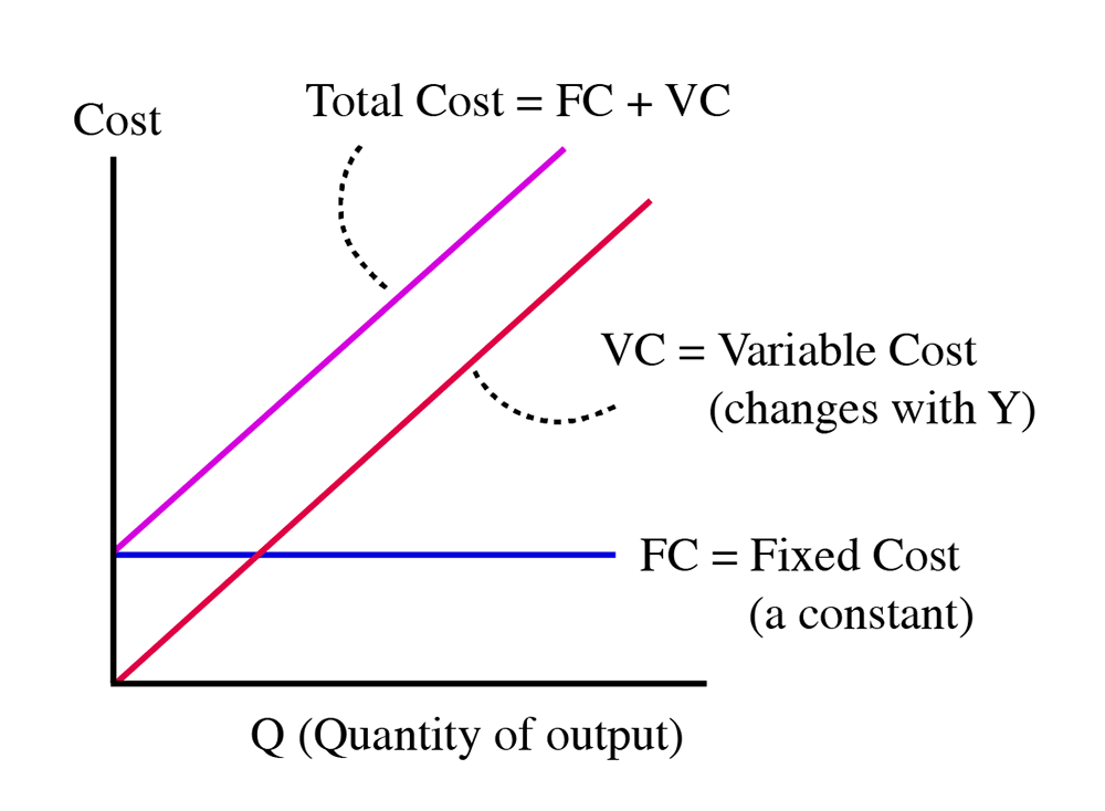
Using abbreviations, we say that .
Average Cost
An average cost is the total cost divided by the quantity:
- . (Can also be labeled as ATC: average total cost)
We can also have average fixed cost and average variable cost:
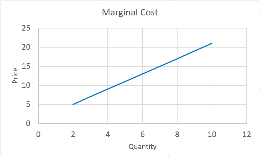
Marginal Cost
Marginal Cost is the most important cost of all. Greg Mankiw, whom we mentioned in the first lesson, calls this the “most important concept in economics.” The marginal cost is the cost of producing one more unit (or can be thought of as the cost of producing the last item). So, it is the change in total cost for some change in quantity:
where TC1 is the total cost of producing Q1 units, TC2 is the total cost of producing Q2 units of output.
We can have the Q1 = Q and Q2 = Q +1 in that case, the Marginal Cost equation will be simplified as:
Example: Assume that the fixed cost for a shoe firm is 500, and it costs 100 to produce each individual pair of shoes. For Q=1 to 10, determine the fixed cost, variable cost, total cost, average variable cost, average fixed cost, and marginal cost.
| Q | FC | VC | TC | ATC | AFC | AVC | MC |
|---|---|---|---|---|---|---|---|
| 1 | 500 | 100 | 600 | 600.00 | 500.00 | 100 | 100 |
| 2 | 500 | 200 | 700 | 350.00 | 250.00 | 100 | 100 |
| 3 | 500 | 300 | 800 | 266.67 | 166.77 | 100 | 100 |
| 4 | 500 | 400 | 900 | 225.00 | 125.00 | 100 | 100 |
| 5 | 500 | 500 | 1000 | 200.00 | 100.00 | 100 | 100 |
| 6 | 500 | 600 | 1100 | 183.33 | 83.33 | 100 | 100 |
| 7 | 500 | 700 | 1200 | 171.43 | 71.43 | 100 | 100 |
| 8 | 500 | 800 | 1300 | 162.50 | 62.50 | 100 | 100 |
| 9 | 500 | 900 | 1400 | 155.56 | 55.56 | 100 | 100 |
| 10 | 500 | 1000 | 1500 | 150.00 | 50.00 | 100 | 100 |
Practice Exercise
Assume the fixed costs for a pizza restaurant is 150 and it costs 15 to produce each pizza. For Q=1 to 10, determine the fixed cost, variable cost, total cost, average variable cost, average fixed cost, and marginal cost.
Example
When we mathematically represent a cost function, it might look something like this:
So, you will know that the Fixed Cost is the constant term (the term that does not include any mention of Q), and the Variable cost is the sum of all of the terms that include Q in some way. If a term does not include Q, then, clearly, it does not change when Q changes:
An average cost is the total cost divided by the quantity:
We can also have average fixed cost and average variable cost:
We can use the following equation to calculate the Marginal Cost, for example
Then, the total cost of producing 10 units will be given as:
Using the same function, the total cost of producing 11 units (one more unit) will be:
So, the marginal cost of the 11th unit =
Note: .
So, by canceling out the FC term, we get , and we can say that:
Of course, anything defined in discrete difference (“delta”) terms can also be described in continuous terms by using a derivative:
Practice Exercise
Following the previous example, for Q=1 to 15, determine the fixed cost, variable cost, total cost, average total cost, and marginal cost. Then try to draw the graph including the cost metrics.
Take Aways
After working through the material on this page and reading the associated textbook content, you should be able to confidently:
- define and calculate the following terms:
- fixed cost, average fixed cost
- variable cost, average variable cost
- total cost, average total cost
- marginal cost
- derive the fixed cost, variable cost, average costs and marginal cost when given a total cost function.
Supply Curve
Everything in the realm of costs that we have talked about - returns to a factor, fixed and variable costs, economic profits - help define the supply curve.
What is the supply curve? Like the demand curve, it is a Functional Relationship. It is a relationship between the amount of money a firm is willing to accept in exchange for a certain amount of some good. It is not a constant. Because of the notion of declining marginal returns, we can assume that as we produce more of a good, the marginal cost of that good increases. This means that supply curves slope upwards. According to the law of supply, there is a positive relationship between the price of a good or service and the amount of it that suppliers are willing to produce. Meaning that if price increase, producers will supply more.
In reality, most marginal costs curves are U-shaped - they start very high at low volumes of production, they decrease as more of a good is made (economies of scale), and then as diminishing returns kicks in, the curve starts to rise again. There are some industries in which the marginal cost - that is, the cost of serving one more customer - continually slope downwards, like the utilities.This is a special case we will talk about later.
So, the supply curve is a relationship that tells us the minimum amount that a firm is willing to accept for selling a unit of a good. What is this minimum amount? Well, if you are a firm and you need to make one more unit of a good, then the cost to you of that good is the marginal cost of that good. To make the good, you need to recover, at a minimum, your marginal cost. Therefore, the supply curve IS the marginal cost curve.
First, we need to find the and . We can do that using supply function:
We can find the total cost and marginal cost for Q=1 to 10 as:
| Q | TC | MC |
|---|---|---|
| 1 | 8 | |
| 2 | 13 | 5 |
| 3 | 20 | 7 |
| 4 | 29 | 9 |
| 5 | 40 | 11 |
| 6 | 53 | 13 |
| 7 | 68 | 15 |
| 8 | 85 | 17 |
| 9 | 104 | 19 |
| 10 | 125 | 21 |
Individual Supply Curve
Following graph displays the marginal cost (price) on the y-axes versus quantity on the x-axes. This curve is the supply curve (function) for the supplier. As we can see, it is an upward line. So, in order to find the supply curve (function), we need to extract the marginal cost from the total cost function. This graph tells us if price is $15, this producer is willing to produce 7 unites of the good. Or, for example, the minimum amount of money that this producer is willing to exchange for producing 4 units, is $9.
Note that market supply curve is the summation of all individual producer supply curves.
Producer surplus
Similar to the concept of consumer surplus that we learnt in Lesson 2, we can define the producer surplus. Let’s start with an example. Assume you own a pizza shop and you are willing to make and sell pizza if price is at least $1.5 per slice. However, the market price is $2 per slice and you can sell each slice at the market price and receive $2. The difference between $2 and $1.5 is your net gain from exchanging the pizza with money. This gain is called your producer surplus. Producer surplus is the difference between minimum price you are willing to make and sell, and the amount you actually receive from selling the pizza. Please note that this gain is different from profit.
Let’s assume market production for a good equals
So, if the market price is $20, market will supply 8 unites of the good . And we know that is the market supply function, which is the summation of all individual supply functions.
Let’s say the first producer is willing to supply the first unit of the good to the market at the price of 6 dollars (you can plug Q=1 to the supply function). However, the market price is $20. So, his individual gain (individual producer surplus) from producing and selling, will be $14 . And if we do this for all other unites of the good, we can find the individual producer surplus for other suppliers in the market. And if we add them all together, we can calculate the total producer surplus in the market.
You might have already noticed that for finding the total market producer surplus, we just need to find the area of the triangle, which is bounded to supply curve, market price (horizontal line), and the y axis.
For calculating the area, we need to find the length of two sides :
A represents the market price and the coordinate will be (0, $20)
B is the supply curve intercept and the coordinate will be (0, $4)
C is the market supply at price = $20, and you can find the coordinate simply by plugging P=20 into the supply function . And the coordinate of C will be (8, $20)
Now that we have the coordinates, we should be able to calculate the area of triangle as:
So, producer surplus at market price of P=$20 will be 64.
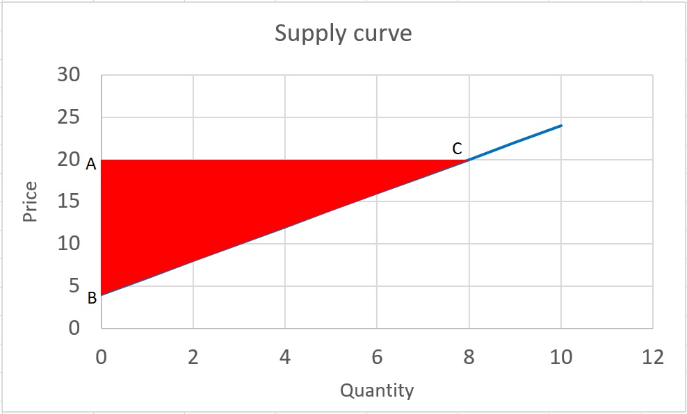
Note that, in general, when we are talking about the producer surplus, we refer to the market producer surplus, which is the summation of all individual supplier producer surplus. So, to calculate the producer surplus, we need to find the area above the supply curve and below the price. This area represents the total producer surplus in the market.
Price elasticity of supply
Similar to the method that we used to calculate the price elasticity of demand, we can define and calculate price elasticity of supply as:
“Percentage change in quantity supply, divided by percentage change in the price causing the supply response.”
The Greek letter eta is used to denote elasticity.
Price elasticity of supply reflects the sensitivity of suppliers to the price changes. Note that, since supply curve is upward, the price elasticity of supply is a positive number.
Example: Following the previous example find the elasticity of supply when price increase from $20 to $24.
First, we need to find the and . We can do that using supply function:
We can also calculate the midpoint elasticity as:
Investments and Economic Profits
We spoke in the last lesson about profits. So, what are profits? They are defined as revenues minus costs, or the money left over after all of the bills have been paid.
Where do they go? Every firm has an owner, and these owners are the people who legally own the profits from the firm. People invest (put in) their money, their time and their effort in a firm with the hope that the firm will make a profit. Therefore, the profit is a payment to the owner of the firm in exchange for the things he has put into the firm. In a small business, the owner puts in time, money and effort. In a large, public share company (called a joint-stock company), owners only put in money when they buy shares. So, the money left over after operations, which is total revenue minus total costs, is what we call the "accounting profit," and this is the payment to the owner in exchange for making an investment in that firm.
How much profit should a firm make? To think about this, it is helpful to think about some choices you have as an investor. Let us imagine that there is an investment that is 100% safe. This means that you know for sure that this investment will pay the profit it promises to pay.
Let’s say this safe investment promises to pay 5% profit after 1 year.
Now, imagine another investment which is not 100% safe. In fact, 10% of the time, this investment vanishes into nothing. How much profit would this investment have to make to want cause you to invest? Phrasing this another way, what kind of earnings would you have to make on the "unsure" investment to make you indifferent to choosing it or the "safe" investment? By indifferent, we mean that you do not care between one or the other, because they are essentially the same thing. This is where we start delving into notions of probability, uncertainty, and expectations about the future.
Well, let us do the math:
For the safe investment, you will get back $105 for a $100 investment today.
For the other one, you will get $0 back 10% of the time, and $100 + X back 90% of the time. X is the profit (interest) on the risky investment. What does X have to be to make these two choices the same?
So, if this other investment pays a profit of $16.67 on $100, then you should be indifferent to the two investment choices. That is, the two investments have the same Expected Profit to the investor.
Yield
When expressed as a percentage gain, this profit is called the Yield from the investment. In the above example, the yield from the second investment has to be at least 16.67% for you to be interested in making that investment. If it is higher (say, 20% yield), then you would prefer it to the safe investment. If it is lower (say, 10% yield), then you would prefer the safe investment.
Risk
Why does the second investment have to pay a higher yield? Because there is a chance that the investment will fail and pay you back nothing. This is what is called Risk. Risk is another word for Uncertainty: the lack of knowledge of what will happen in the future.
The profit from every investment has two parts: the risk-free return, and the risk premium.
Risk-free Return (RFR)
Risk-free return (RFR) is the profit you can make from an investment that has absolutely NO uncertainty. You know, for sure, that you will get paid a promised profit. Is there a risk-free (100% sure) investment? No. But there is one that is very close: lending your money to the US Government. The US Government borrows money by printing up pieces of paper called Treasury Bills (T-Bills). These are promises to pay a certain amount of money at some point in the future. For example, a T-Bill might promise to pay $100 one year from now. If you buy this T-Bill for $95 today, you are making a yield of 5.26%.
This is considered to be the safest investment in the world. The chance that the US Government will not pay the promised amount on its T-Bills is considered to be so close to zero as to be equal to zero. So, for any investment, the risk-free rate is the return a person could get from buying US T-Bills.
Risk Premium (RP)
Risk premium (RP) is the amount of profit that is paid to compensate for the chance that the investment will disappear. In the example shown above, the risk premium is equal to 16.67% - 5% = 11.67%. Because there is a 10% chance that your investment will vanish, the owner of the firm will have to promise to pay you an extra 11.67% IN ADDITION TO the risk-free return in order to get you to take the risk. The riskier the investment (that means, the higher the chance the investment will vanish) the higher the risk premium that has to be paid.
Risk versus Reward
Risk versus reward is an underlying concept of the capitalist system: that a person who takes a higher risk expects a higher return. Thus, risk-takers are often people who make a large amount of money, but only after they have lost their money several times. The higher the risk in an investment, the higher the risk premium.
Expected Profit and Economic Profit
The expected profit from an investment is the risk-free return (RFR) plus the appropriate risk premium (RP) for the industry in question. So, the accounting profit (TR – TC) should be equal to (RFR + RP). If the profits are greater than (RFR + RP) then we say that an investment is making an Economic Profit. This means the firm is paying a yield that is greater than the yield for other companies with similar risk. We expect economic profits to always be moving towards zero. The reason for this is simple: if an investment is paying an economic profit, it is basically paying out “free money,” more money than a similar investment. So, what happens? Everybody will move into the “good” investment. There will be more demand for this investment. More demand means the price will go up, which means the yield will shrink. (Remember, yield = (future payment – purchase price)/purchase price. As purchase price goes up, yield goes down.)
This is the theory of Efficient Markets. This means that if there is a very good investment, everybody will want to invest in it, making it more expensive, and therefore making it less of a good investment. So, in the long run, we expect every economic profit to be pushed towards zero. The only way a firm or person can make positive economic profits over time is to keep their profits secret or their methods secret, and both of these are very difficult to do.
Think of the idea of opportunity cost. The opportunity cost is the value of the most valuable thing you did not do. So, when you invest your money, you will discover that there are many, many places where you can put your money. Which is the best one?
The profit you expect to make from an investment should be at least as good as the next best possible choice. So, the economic profit from an investment is the difference between the best choice and the next-best choice.
For this reason, we always expect the economic profit to be zero. Or, at least, moving towards zero.
Example
Let’s say there are two choices of investment in firms in the same industry. In this industry, the risk-free return is 5% and the risk premium is 5%:
Buy stock in company A for $100 per share and earn $10 per year in profit.
Buy stock in company B for $60 per share and earn $9 per year in profit.
The profit on investment B is 15%, but in company A it is 10%. So the economic profit from owning B will be 5%. But, because of this, everybody will want to buy B. When the demand for a good increases, the price goes up, and in this case, the price will go up until the percent profit is the same as company A. The economic profit will be driven towards zero.
This helps us define how much profit a firm "should" make. In the first lesson, I counseled against "should" statements, because they are normative statements, and as objective and disinterested observers of the real world, we are only interested in "positive" statements. So maybe we can rephrase the question: how much profit does a firm have to make in order to make it an attractive investment? Well, we know that it has to make at least the risk free rate plus the risk premium. If it is making exactly this amount, it is making zero economic profit, and the investor should be indifferent to this investment and all others that make zero economic profit. If it is making more than zero economic profit, it is a very attractive investment, and because a lot of people will want to get at the "free money" that this firm is making, the stock price should go up, driving the economic profit to zero. The opposite will happen to a firm that is making negative economic profits.
The textbook author talks about "explicit" and "implicit" costs - explicit costs refer to things that a firm has to purchase in order to operate - paying wages to staff, purchasing raw materials and energy, paying rent and taxes, and so on. The other type of costs are implicit, and these refer to the use of the owner's resources - the owner's time and effort. This is the "return to the owner" I spoke of above. The return to the owner is equal to the opportunity cost of his/her time - the value of the best alternative use. Any business enterprise should be compensating the owners of the firm at a level that at least matches the opportunity cost of capital, on a risk-adjusted basis. If it does not, it makes more sense for an owner to invest elsewhere.
This informs us about the cost structure of a firm. When a firm is selling its product, it has to be selling at a price that is high enough to ensure accounting profits sufficient to generate enough of a return to cover the risk-free rate plus the risk premium - the payment that the owner must get in return for investing his money in the firm.
Take Aways
After working through the material on this page and reading the associated textbook content, you should be able to confidently:
- define accounting profit;
- define economic profit and understand its difference from accounting profit;
- understand what we expect economic profit to be, and why;
- understand the concept of risk in an investment;
- know what the two parts of profit from an investment are;
- understand what a risk premium is, and where it comes from.
Summary and Final Tasks
In this lesson, we described the source of the supply curve, which is basically a functional relationship that defines the minimum amount of money a firm can charge for a certain amount of some good it is selling in a market place.
It turns out that the supply curve is defined by the marginal cost of a good, which means that if a firm makes one more unit of a good, they must be willing to sell it for at least the cost of making that unit. Included in the marginal cost is an amount that is equivalent to a necessary return to an owner, sufficient to make a person want to invest in a certain industry. This is the amount that yields "zero economic profit," which simply means that a firm in a specific industry is generating an accounting profit that is sufficient to provide a return on investment that equals the risk-free rate plus the appropriate risk premium for the industry in question.
When the supply curve is plotted on the same diagram as a demand curve, we have a "supply and demand" diagram, and the point at which the supply and demand curves intersect is called the "market equilibrium." It is the price and quantity sold that we expect to see in a perfectly competitive market at a given point in time.
A perfectly competitive market is one in which our four assumptions of perfect competition are met:
- No market power
- Perfect information
- Product homogeneity
- Free entry and exit
These four conditions are rarely met in real life. Any deviation from this condition is called a "market failure." We will spend much of the rest of the course studying market failures, and the problems that are associated with governments trying to fix market failures, which we call "government failure."
Have you completed everything?
You have reached the end of Lesson 3! Double check the list of requirements on the first page of this lesson to make sure you have completed all of the activities listed there.
Tell us about it!
If you have anything you'd like to comment on or add to the lesson materials, feel free to post your thoughts in the discussion forum in Canvas. For example, if there was a point that you had trouble understanding, ask about it.