Course Outline
Lesson 1 - The Energy Industry – Overall Perspective
Lesson 1 Introduction
Overview
As the saying goes, “the only constant is change.” This statement can be used to describe the energy industry over the past few decades. “Booms” and “busts” have occurred numerous times as prices rose and then fell back again. Companies have come and gone. Enron shook the very foundation of energy trading. Investigations of supply and price manipulation have occurred, resulting in fines and imprisonment. The new exploration ("3-D & 4-D" seismic), drilling (directional & horizontal), and completion techniques (so-called “fracking”) have not only led to a substantial increase in the production of crude oil and natural gas, but have also led to great controversy and new regulation over the methods themselves. The abundance of natural gas is leading to the exportation of liquefied natural gas (LNG), making the US a major player in that global market.
The “how” and “why” these occurred will be presented throughout the course, and you will come to understand the ever-changing landscape that is the energy industry in the United States.
Despite the reference to alternative & renewables energy sources in the course description, we will spend very little time discussing them. This course focuses largely on the five fossil fuels that are traded both physically and financially in energy markets. These are natural gas, crude oil, unleaded gasoline, heating oil, and natural gas liquids (NGLs). The reason for this is that these energy commodities are heavily traded in financial futures markets. Understanding how these financial markets work is the primary goal of this course. These fuels, along with coal, comprise the “non-renewable” energy sources. They are so named since their supply is seen as finite over the long-term. Then we will extend our knowledge to the electricity market, its characteristics, and differences. We will also introduce the risk management methods.
Each of these products has a profound effect on the United States and global economies. Billions and billions of dollars of infrastructure and hundreds of thousands of jobs are involved in the exploration, production, transportation, and distribution of these forms of energy. And price volatility for these commodities has increased dramatically over the past several years going back to the historic run to $147 per barrel (Bbl) for oil in 2008. Since that time, crude oil has been recognized as a truly global commodity with a host of new factors influencing price. And, once again, in 2014, prices fell from $100 in June to less than $50 by December, caused largely by Saudi Arabia flooding the market with cheap crude. It was said they feared a loss of market share to the new shale oil in the US. One of the major players in the oil market is Organization of Petroleum Exporting Countries (OPEC), with about 40 percent market share of the world's crude oil production. OPEC decisions and members' agreement have a substantial effect on crude oil price. Following the oil price drop in late 2014 and 2015 to about $30/Bbl, OPEC members (and some other producers) came to an agreement to decrease their production, which caused the prices to increase in late 2016 and 2017. In March 2020, following the global pandemic, crude oil futures price dropped to about - $40/bbl for the first time in history.
However, before we proceed into the details of these fossil fuels, we need to understand how these fit into the overall profile of energy production and consumption in the United States. In order to do this, we must also include the various other forms of energy produced and consumed in the United States, known as “alternative” and “renewable” energy. This is the only lesson regarding alternative and renewables.
Learning Outcomes
At the successful completion of this lesson, students should be able to:
- describe the major sources of energy in the United States;
- outline the energy production/consumption environment;
- explain what is meant by “renewable” vs. “non-renewable” energy;
- evaluate the pros and cons of 5 different types of alternative fuels, including the cost to produce, emissions profile, feedstock, and likelihood of increased use;
- list the main fossil fuels;
- critically assess the pros and cons of each type.
What is due for Lesson 1?
This lesson will take us one week to complete. The following items will be due Sunday at 11:59 p.m. Eastern Time.
- Introduce Yourself discussion
- Lesson 1 activities as assigned in Canvas
Questions?
If you have any questions, please post them to our General Course Questions discussion forum (not email), located under Modules in Canvas. The TA and I will check that discussion forum daily to respond. While you are there, feel free to post your own responses if you, too, are able to help out a classmate.
Reading Assignment: Lesson 1
Optional Readings
Lesson 1 doesn't have any reading assignments. However, the following readings are optional and recommended.
- Wind Power [1]
- Hydropower [2]
- Solar Energy [3]
- Geothermal Energy [4]
- Biomass [5]
Major Sources of Energy in the United States
“Non-renewable” energy sources (such as Oil and Petroleum Products [6], Natural Gas [7], Natural Gas Liquid [8], Coal [9], and Nuclear [10]), as well as “renewable” energy and “alternative fuels” (such as Hydro [2], Solar [3], Wind [1], Geothermal [4], Biomass [5], and Biofuels [11]), help to satisfy the nation’s energy needs. Fossil fuels and nuclear power are considered non-renewable sources of energy. Coal and natural gas play large roles in the generation of electricity as well as in industrial processes such as the manufacturing of steel. Hydro, solar, wind, biomass, biofuels, and geothermal are all considered “renewable” forms of energy and comprise varying levels of supply in this country. They are classified as renewables since their source is seen as being virtually unlimited. Of these, solar, wind, biomass, biodiesel, and geothermal are all considered “alternative” energy sources since they are not the “traditional” kind (fossil fuels, nuclear, and hydro).
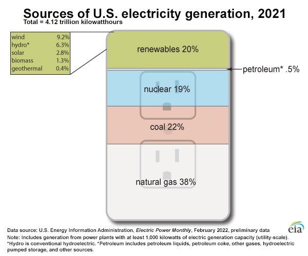
The following chart is from EIA reported data [12] and shows major energy sources and percent shares of U.S. electricity generation at utility-scale facilities in 2021. Please note that in 2021 natural gas has the largest share (38%) in U.S. electricity generation, coal is in the second place (22%), and nuclear has the third place (19%). As shown in Figure 1, renewable energy sources contribute to about 20% of the U.S. electricity production at utility-scale facilities as of 2021, with about 9.2% wind power and 6.3% hydro. Please note that 2019 was the first year that wind power surpass the hydro. Other renewable sources such as solar, biomass and geothermal have a minor share.

U.S. Electricity Generation in 2019
Total = 4.009 trillion kilowatthours (kWh)
-
Natural Gas: 40%
-
Nuclear: 20%
-
Coal: 19%
-
Renewables: 20%
The renewables are broken down as follows:
-
Wind: 8.4%
-
Hydropower: 7.3%
-
Solar: 2.3%
-
Biomass: 1.4%
-
Geothermal: 0.4%
Figure 2 below shows the break-out of fuel sources used in the generation of electricity. As you can see, the single largest fuel has been coal in the past decades, although this is changing as historically low natural gas prices during 2010-2020 caused some “fuel switching.” This was followed by natural gas, nuclear, and renewable energy sources. This final category is comprised of energy sources such as wind, solar, hydroelectric, biomass, and geothermal.
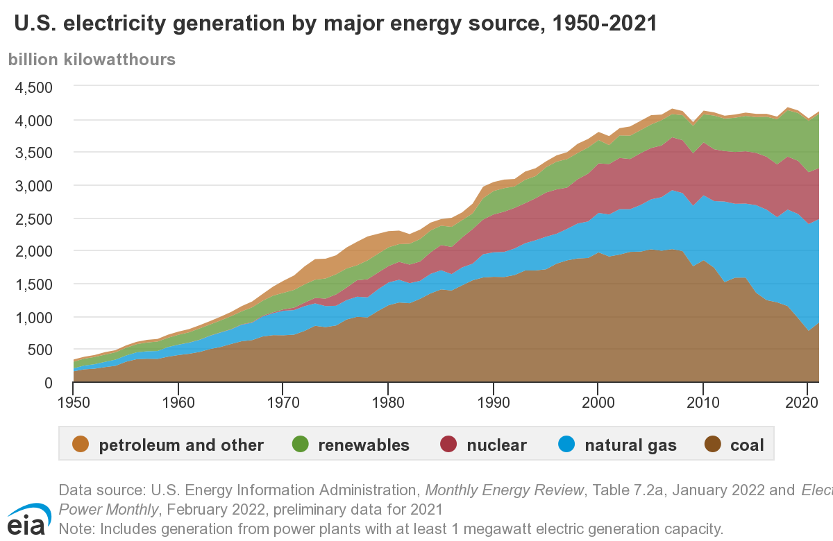
Figure 3, below, displays the renewable energy sources that contribute to power generation. As you can see, there has been a rapid increase in wind and solar power generation. However, it will take decades for alternative fuels to make a substantial contribution to the energy portfolio in the United States. Thus, there is a need to continue to use fossil fuels and nuclear power to “bridge” the gap. How the former (fossil fuels and nuclear power) are delivered to market and how they are priced is the main focus of this course.
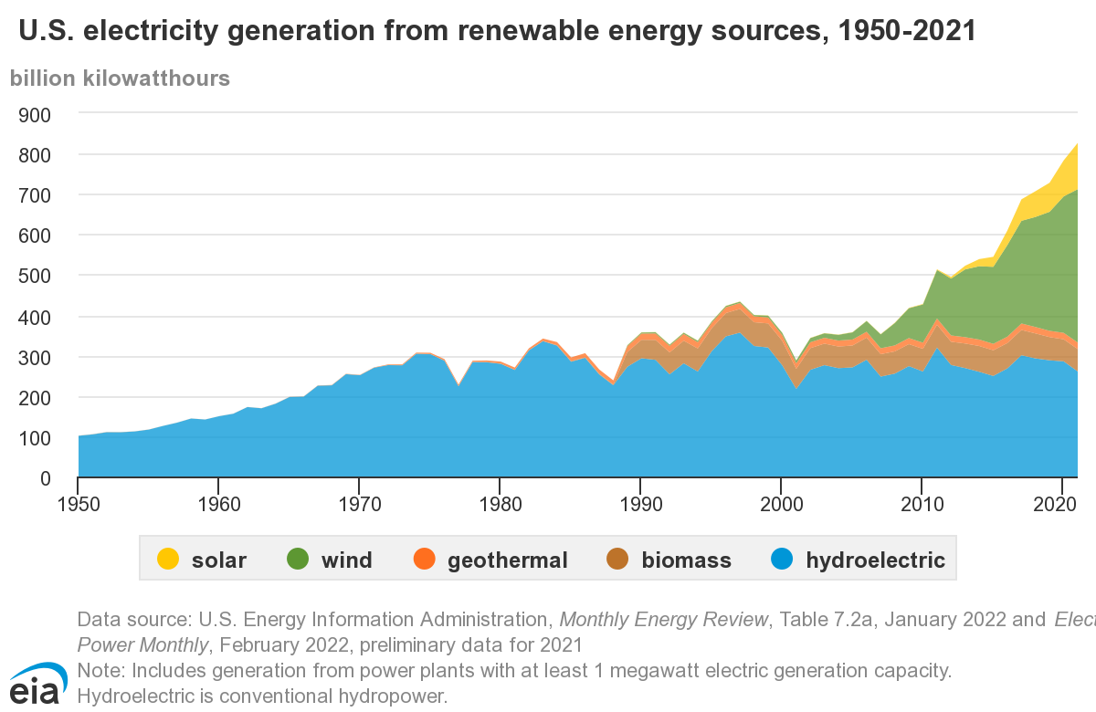
Renewable electricity generation
1950 - 2020 (history)
Geothermal: Geothermal generation was relatively stable, and very low, from 1990 - 2020.
Biomass: Biomass generation has remained steady at about 50 - 60 billion kWh from 1990 - 2020.
Hydroelectric: Hydroelectric generation varied widely between about 220 billion kWh and 350 billion kWh from 1990 - 2021.
Utility-scale and end-use solar: Solar generated almost zero kWh before 2010. It rose from almost zero to about 115 billion kWh by 2021.
Wind: Wind power generated almost no power until 2004. From 2004 until 2021 it rose to about 378 billion kWh, more than 25 times of 2004 generation level.
- Geothermal: Geothermal generation was relatively stable, and very low, from 1990 - 2020.
- Biomass: Biomass generation has remained steady at about 50 - 60 billion kWh from 1990 - 2020.
- Hydroelectric: Hydroelectric generation widely between about 220 billion kWh and 350 billion kWh from 1990 - 2021.
- Solar: Utility-scale and end-use solar generated almost zero kWh before 2010. It rose from almost zero to about 115 billion kWh by 2021.
- Wind: Wind power generated almost no power until 2004. From 2004 until 2021 it rose to about 378 billion kWh, more than 25 times of 2004 generation level.
Now that we have clarified the difference between renewable and non-renewable sources of energy, let’s have a look at the production and consumption of energy in the United States on a macro level.
Energy Production and Consumption in the United States
The United States is the world’s largest consumer of energy in general and of oil and refined products in particular. However, our current and forecasted energy production and consumption balance is improving towards a position of declining imports and more efficient use of all energy sources. The vast new supplies of oil and natural gas coming from domestic shale are radically altering our outlook for eventual self-sustainability. And the continuing development of “renewable” and “alternate” energy sources will decrease our reliance on traditional “fossil” fuels. We will now take a look at the current state of energy production and consumption in the US, followed by a brief examination of the renewable and alternative energy sources.
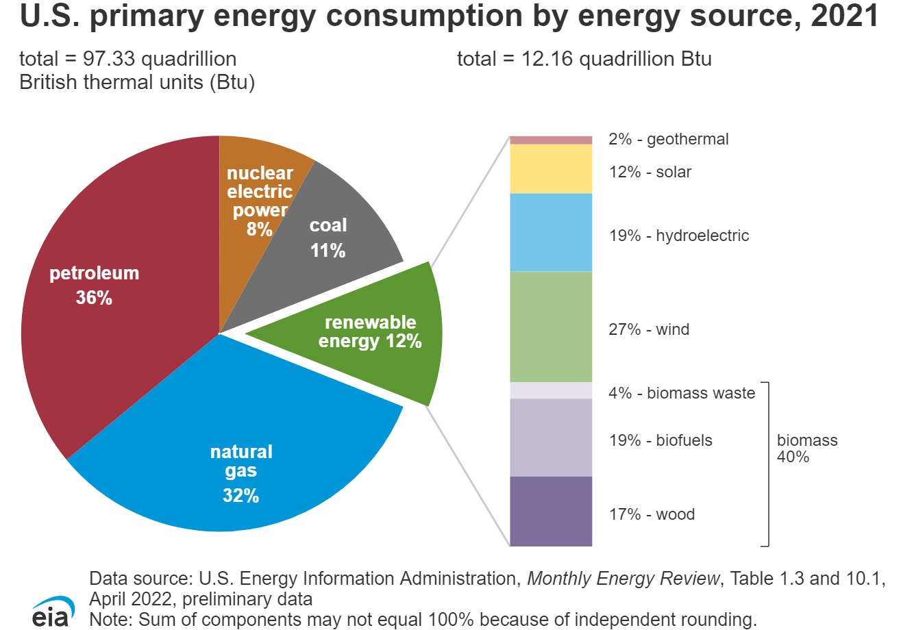
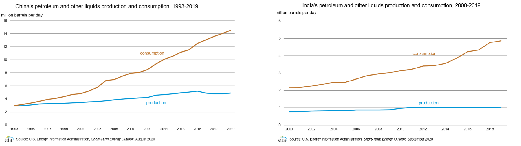
The following pie chart (Figure 4) shows the United States' energy consumption by source in 2021. As shown in the chart, petroleum that is mainly used for the purpose of transportation has the biggest share of 36%. Natural gas is in second place with 32% share of energy consumption.
U.S. Energy Consumption by Energy Source, 2020
Total = 100.2 quadrillion British thermal units (Btu)
- Petroleum: 37%
- Natural Gas: 32%
- Coal: 11%
- Nuclear electric power: 8%
- Renewable Energy: 11% (10.2 quadrillion Btu)
Renewable energy is broken down as follows:
- Hydroelectric: 22%
- Biomass: 43%
- Wood: 20%
- Biofuels: 20%
- Biomass Waste: 4%
- Wind: 24%
- Solar: 9%
- Geothermal: 2%
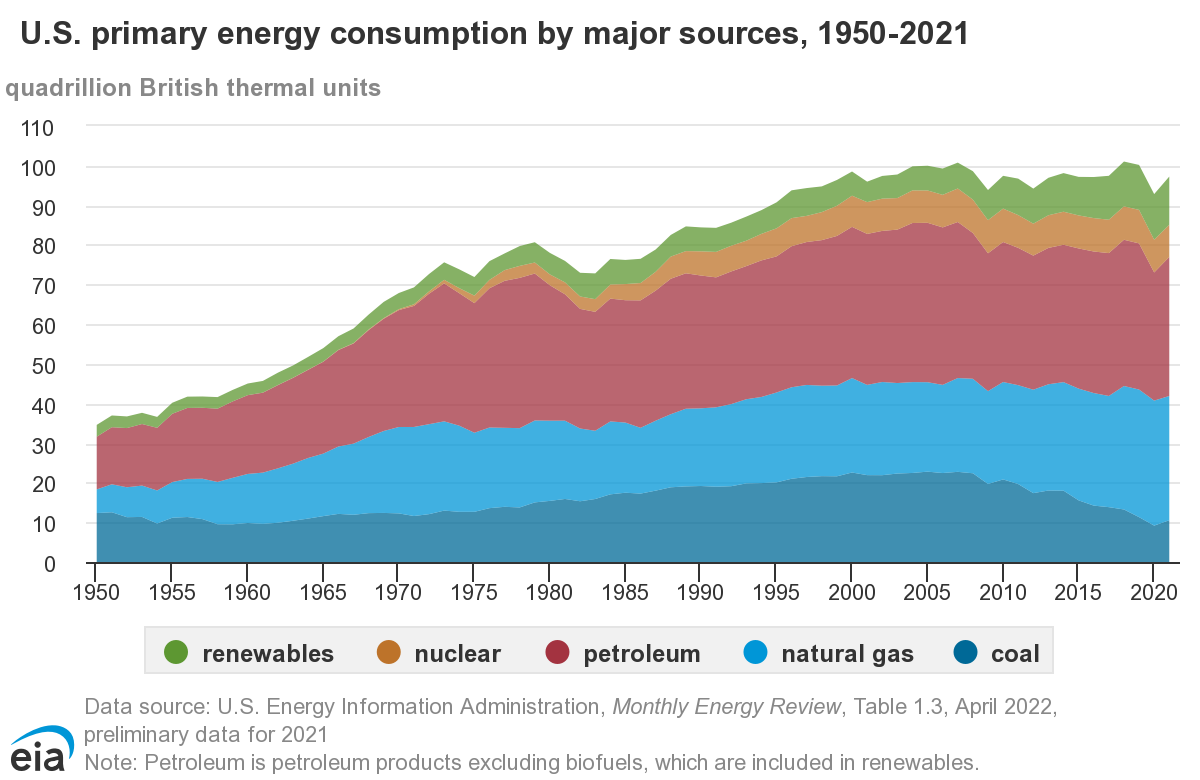
Figure 5, below, illustrates the historical energy consumption in the United States by source. Notice the decline in the use of coal, while natural gas and renewables consumption are increasing. The increase in natural gas consumption has much to do with the following: the current historically low prices resulting from the huge amount of new shale gas being produced, and new tighter emissions standards being imposed on coal-fired power plants. If you are interested to see the historical trend by the source, individually, click on the following link, it is a graph showing the history of energy consumption in the United States from 1750 to 2015 [15].
Alternative energy sources will continue to grow as long as economically feasible, and especially if government subsidies are available to support their production (e.g., – ethanol). Note that EIA publishes annual reports for the US Energy Outlook, which include future projections. If you are interested in the projected energy outlook in the United States, click here [17]. You may notice EIA (Energy Information Administration) is projecting a significant increase in production and consumption from renewables by 2050. While, nuclear production is shown as being stable, and with the negligible emissions they produce.
In addition, as far as natural gas goes, an increase is indicated. The residential use of heating oil and propane is steadily declining as conversions to natural gas steadily continue. (50% of US homes use natural gas for space heating and hot water.) Add to that the retirement of coal plants, or the outright switching from coal to natural gas, and growth in the consumption of natural gas will naturally occur.
The future consumption of oil and “other liquids” will be interesting to observe as well. With automobile efficiency improving and electric cars gaining in popularity, this segment should decline. Also, there are decades-old power plants, mostly in the Northeastern US, that use fuel oil. These, too, will become obsolete or convert to natural gas. (The Northeast US is also the world’s largest consumer of heating oil.)
There should also be a more dramatic decline in the use of coal than what is shown above, as emissions restrictions and lower natural gas prices make coal less economic to use.
The fuels we will study in-depth, natural gas and “oil and other liquids,” comprise more than half of the projected total US energy consumption profile, thus making it crucial to understand the logistics and “value chain” of these fuel sources.
The following chart illustrates the various types of energy in the US and the corresponding consumption types.
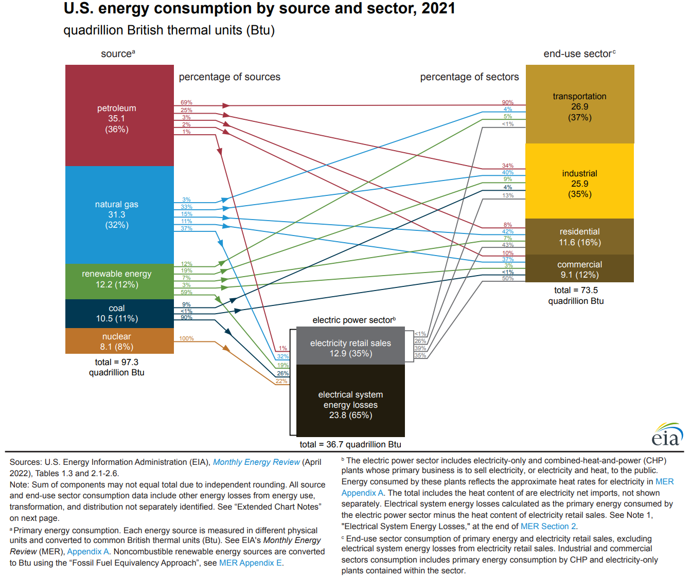
Energy Sources
Petroleum (37%)
70% of the petroleum goes to the Transportation Sector
24% of the petroleum goes to the Industrial Sector
5% of the petroleum goes to the Residential and Commercial Sector
1% of the petroleum goes to the Electric Power Sector
Natural Gas (32%)
3% of the Natural Gas goes to the Transportation Sector
33% of the Natural Gas goes to the Industrial Sector
27% of the Natural Gas goes to the Residential and Commercial Sector
36% of the Natural Gas goes to the Electric Power Sector
Coal (11%)
10% of the coal goes to the industrial sector
<1% of the coal goes to the residential and commercial sector
90% of the coal goes to the Electric Power Sector
Renewable Energy (11%)
12% of the renewable energy goes to the Transportation Sector
22% of the renewable energy goes to the Industrial Sector
9% of the renewable energy goes to the Residential and Commercial Sector
56% of the renewable energy goes to the Electric Power Sector
Nuclear Electric Power (8%)
100% of the nuclear electric power goes to the Electric Power Sector
Energy Consumption by Source
Transportation (28%)
91% of the energy used in this sector comes from petroleum
3% of the energy used in this sector comes from natural gas
5% of the energy used in this sector comes from renewable energy
Industrial (26%)
34% of the energy used in this sector comes from petroleum 40% of the energy used in this sector comes from natural gas 4% of the energy used in this sector comes from coal 12% of the energy used in this sector comes from renewable energy
Residential and Commercial (about 20%)
9% of the energy used in this sector comes from petroleum
42% of the energy used in this sector comes from natural gas
<1% of the energy used in this sector comes from coal
45% of the energy used in this sector comes from renewable energy
Electric Power (37%)
1% of the energy used in this sector comes from petroleum
38.4% of the energy used in this sector comes from natural gas
23.5% of the energy used in this sector comes from coal
17.5% of the energy used in this sector comes from renewable energy 2
19.7% of the energy used in this sector comes from nuclear electric power
In Figure 6, above, we see the energy sources matched-up with their respective categories of consumption. Both petroleum and natural gas are used in each sector of consumption, while coal is utilized in only industrial, residential (this would have to be a very small amount), and power generation. Nuclear energy is strictly used for electric power generation, and renewables can be consumed in all categories but contribute very little to each on a percentage basis.
The sources and uses of energy are important for the overall understanding of the impact of supply, demand, and pricing on the macroeconomic environment. Everything depends on energy, and understanding these interrelationships can help us manage our supply needs and price exposure.
Global energy use and trade
So far, we have examined the energy portfolio of the United States, and next, we will take a look at the global energy production and consumption as well as the energy profiles of several major countries.
Figure 7 shows the total energy consumption of the world by sources over two centuries. Until the mid-19th century, traditional biomass, like the burning of wood, crop waste, or charcoal, was the dominant source. With the Industrial Revolution, coal replaced traditional biomass as the dominant one, and then was replaced by oil in the 1960s. Natural gas, nuclear, and hydropower were added to the mix around the same period. Solar and wind came much later in the late 1980s. A fast expansion of natural gas and renewables has been ongoing since the 21st century. Compared to the energy portfolio of the U.S., the worldwide reliance on fossil fuels is much greater, where more than 77% of energy demand is met by oil, natural gas, and coal. It is also worth noting that traditional biomass is still one of the major sources for many developing regions.
Figure 8 shows the 2021 energy consumption by country. Here we briefly introduce energy portfolios and energy import/export of several major counties/regions.
- China is the top energy consumer in the world, due to its 1.4 billion population and economic growth in recent decades. Coal is the major energy source for China, mainly for electricity generation, steel and cement manufacturing, and residential heating. It is the second largest crude oil consumer (after the U.S.) and third in natural gas. Due to limited domestic supply, it is the top importer of both crude oil and natural gas. Renewables are developing fast in China, helping its target of reaching CO2 emissions peak before 2030 and achieving carbon neutrality by 2060.
- India is the third energy consumer, with a similar size of population as China. Coal is its largest source, but not as large as China. Traditional biomass is still contributing to a substantial but falling portion of energy, while renewables are supplying a very minor portion of energy. India is the third in crude oil consumption and import, while not in the top 10 in terms of natural gas consumption and import.
- Japan, with 126 million population, ranks fifth in energy consumption. Nuclear was one of its major sources, providing up to 13% of total consumption, but has fallen to 3% after the earthquake and tsunami near Fukushima. The share of nuclear was replaced by natural gas, oil, and renewables. Currently, petroleum is its major energy source, providing 40% of energy consumption. As an island country, Japan heavily relies on imports for its fossil fuel supply. It is the fifth in crude oil import and the second in natural gas import.
- European Union (EU) is another region that heavily depends on energy imports to meet its demand. It is worth noting that energy profiles vary across different countries. For example, renewables account for over 35% energy supply in Finland, Denmark, and Sweden while nuclear is the major source (40%) in France. Overall petroleum is the major source for the EU (34.5%) and natural gas comes after (23.7%) as of 2020. A substantial amount of energy products was imported from Russia but now EU is exploring other sources like the U.S.
- Russia is the fourth in energy consumption, and contrary to previous energy net import countries and regions, it is the second largest country in crude oil export (after Saudi Arabia) and the largest in natural gas export as of 2021. Russia has the largest proven natural gas reserves in the world and natural gas is also its major source of energy (51% of consumption).
Figure 9&10 shows the top 10 importer and exporter countries of crude oil and natural gas. Top importers are major economies while exporters come from all over the world. As we will see in the following lessons, these countries will have significant impacts on the demand and supply in the world energy commodity market.
Mini-Lecture: Alternate and Renewables
So, what are the “renewables and alternate” sources of energy? As previously mentioned, “renewable [18]” energy sources are those which can be replenished over and over again, such as solar [3], hydro [2], wind [1], biomass [5], biofuels [11], and geothermal [4]. “Alternate” energy sources are those which are not the traditional fossil fuels or nuclear power. These include the renewables: hydro, wind, solar, biomass, biofuels, and geothermal.
As stated previously, it will take a long time for renewable and alternate energy sources to make a significant dent in the US reliance on fossil fuels. In the interim, the fuels we will study in depth, primarily natural gas and crude oil, will continue to be produced and consumed in substantial quantities. Natural gas, as the cleanest burning of the fossil fuels, represents the “bridge” fuel until renewable and alternate energy can be produced in sufficient quantities to wean us of our dependence on fossil fuels.
The following 8:57 minute "mini-Lecture" will cover Alternate and Renewable energy sources in more detail. Mini-Lectures such as this will be provided in most Lessons and will supplement the textual lesson or be the lesson itself. The slides can be found in the Modules under Lesson 1: The Energy Industry - Overall Perspective in Canvas.
Click for a transcript.
This lesson is going to be on alternative and renewable energy sources. The main types that we're going to talk about are wind, hydro, solar, geothermal, and biomass.
Wind power once was used for mechanical drives only. It's gaining in popularity as a clean alternative source of electricity using turbine generators. The old windmills, as they were called, were used on farms to draw water up from aquifers, to serve as wells on their land. And way, way back, they actually ground flour, and corn, and those types of things. Today, large wind farms are being built across the country where wind becomes a natural resource. Some of the concerns with these-- obviously, noise pollution in the area for the residents of that area. And there have been numerous reported deaths to flocks of birds flying in those areas. And as you can see, the picture on the left there just shows what are some 750 kilowatt turbines in the state of Minnesota on a large wind farm there.
Hydropower. Basically using water force as energy. Traditionally, it had been used to churn mills. That's why we would have those water mills. And again, they did several things with those from a mechanical energy standpoint. But today, we have hydroelectric generators. We have, most predominantly, hydroelectric dams. But we also have what are known as tidal power turbines, and these are actually utilizing the current flows, generally in and out of a river, or in and out of some type of an inlet. They use these in the North Sea off of Scotland. There's an experimental one in the East River in New York City as well. Again, there are subsurface turbines that actually spin as the current goes in one direction or another, and those drive a generator, which produces the electricity.
Solar energy has been around for quite some time. The interest in it, and the expansion of it, really began with the oil embargo of 1973 and 1974. And then the second embargo in 1979 caused even more interest in it. The idea is to collect heat and energy from the sun and use it for things such as pure heating, generation of steam for electric turbines, or to actually create electricity directly, which would be the use of photovoltaic cells. In a lot of cases, it's used to heat water, even for space heating.
And we generally have two types. The passive solar energy is using the direct heat of the sun. There are solar collectors, and they can direct the heat in a particular area. It's primarily used for space and water heating, and it can also be used to create steam. So some of the panels you might see on office buildings or residences may be doing nothing more than circulating water through for hot water heating. You would probably recognize the difference or the photovoltaic ones that are producing power.
And again, this brings us to the active part. It's the photovoltaic conversion of sunlight to electricity using semiconductor materials. It's dependent on the atmosphere condition and the Earth's position relative to the sun. And obviously, off to the right there you see a photovoltaic array. Small scale use here. But you see them more and more throughout-- they're using them now for traffic signs, communications systems, for instance pipeline companies, or any type of long distance lines, or cables, or whatever else. Signals are transmitted, and the power is coming from photovoltaic cells.
Geothermal energy. We generally think of geothermal energy as natural steam coming from geysers and from other places. And in those cases, it could be used for direct space heating. It can also be used directly for industrial processes. Steam will also drive steam turbines at a power plant or on site somewhere where there is the geothermal steam coming up.
But the flip side of that, which a lot of people are not necessarily aware of, is the fact that you also have geothermal energy that's used for space cooling. After all, if you go several feet below the surface, the soil and the temperatures down there are much cooler than above ground. And so you can literally drill down into a cooler area and draw up cool air to use for space cooling. This is becoming more and more prevalent. I have personally seen large homes that use this, as well as midsize office buildings.
Biomass. These are the various types when we talk about biomass and energy coming from biomass. We're talking about things like wood, garbage, crops, various alcohol fruits, in other words, fruits that can produce some type of an alcohol that can be burned as energy, and then landfill gas.
Biomass. The one form here is landfill gas. Basically, you have decaying trash that's in landfills, and it's going to create methane. All the biological material that breaks down and decays will end up giving off methane gas, and over time, the older landfills will actually have pockets of methane within them. And there are people who will go out, and they literally will poke a hole down into the landfill, and they will get the pockets of natural gas, and they'll use it on site, mostly. They can use it to drive some small turbines or small generators to create power on site. In some cases, they may have a process whereby they need to create some steam, and so they use the natural gas for that as well.
Another form of biomass is to actually take solid waste and convert it to energy, or trash to energy. This is where using solid waste that would normally go to a landfill-- you're using it as a fuel to create heat via combustion, and in turn, create steam from the boilers where the combustion is taking place. The steam can actually be sold for industrial purposes, or the generation of electricity can be accomplished by using steam as well. Now, there's a company in Fairfield, New Jersey by the name of Cogentrix Corp, and they actually build and operate several of these trash to energy, or solid waste to energy, facilities around the United States.
Wood and wood waste. These are normally the byproducts from large wood mills and paper mills. And what they'll do is, again, to be efficient, and to be environmentally conscious, they'll go ahead and use the wood, or the wood waste, the wood pulp-- they can actually burn it, and then it becomes a heat source where they can create their own steam that they'll use in the process, say, for instance, for making particle board or even paper. They can also use the heat source to run small generators on site for their own consumption and operations. The Weyerhaeuser Company, a huge manufacturer of various forms of lumber, and wood, and particle board, and those types of things, does this on location with a couple of their very large facilities they have in southeast Oklahoma.
And most of us are more familiar with this type of biomass where we're making fuel from things like crops, grasses, and biodegradable matter. One of the more well-known ones, of course, is making ethanol that we use as an additive to gasoline in our cars. And the primary food source there is corn, but there's also sugars that can be broken down into alcohol, as well as certain types of grasses. And on the biodiesel front, we could use vegetable oil, peanut oil, soybean oil, and then recycled grease from restaurants once it's cleaned. You can burn any of these in an existing diesel powered vehicle.
Summary and Final Tasks
Key Learning Points: Lesson 1
Energy consumption in the United States takes many forms. The traditional “fossil fuels,” such as coal, oil, natural gas, gasoline, and other refined products and, natural gas liquids, do not have a limitless supply.
Renewables, however, such as hydro, wind, solar, biomass, biodiesel and geothermal, are self-replenishing.
Alternative fuels comprise the non-traditional energy sources and include nuclear and fossil fuels. Alternative fuels represent the smallest amount of energy consumed in the US and are not expected to expand greatly over the next 20-25 years. And, for many alternative fuels, government subsidies are essential for them to be produced economically.
In the interim, fossil fuels such as natural gas and crude oil will continue to grow in usage and importance. Their supply, demand, and pricing will have a great impact on the US economy for decades to come.
Now that we have examined production and consumption in the United States as well as the energy “mix,” we will focus on the fuel sources that comprise over 57% of the energy used in this country. Crude oil, with refined products, and natural gas and related natural gas liquids (NGLs), make-up this large sector. The factors that influence their supply and demand are varied and ever-changing. Besides the obvious impact of weather, the economy, the US dollar, and the global geopolitical conditions can all influence energy commodities and affect their prices.
Reminder - Complete all of the Lesson 1 tasks!
You have reached the end of Lesson 1. Double-check the list of requirements on the first page of this lesson to make sure you have completed all of the activities listed there before beginning the next lesson. (To access the next lesson, use the link in the "Lessons" menu.)
Lesson 2 - Supply/Demand Fundamentals for Natural Gas & Crude Oil
Lesson 2 Introduction
Overview
In mid-2008, crude oil shocked energy markets as it reached an all-time high of $147/barrel (Bbl.) on the New York Mercantile Exchange. (See Figure 0 below.) Within four months, prices had sunk to $50 per barrel. Then, again in 2014, prices hit a high of about $100/Bbl in June only to fall to under $50/Bbl by December. In April 2020, crude oil futures price dropped to about - $40/bbl for the first time in history. How could these happen, and what were the factors causing these levels of price volatility? We will be exploring these questions in Lesson 2.
Learning Outcomes
At the successful completion of this lesson, students should be able to:
- recognize the various factors impacting supply & demand for natural gas & crude oil;
- research major supply/demand influences:
- global economy,
- domestic economy,
- weather,
- currencies,
- energy commodity relationships,
- inventory and storage reports;
- evaluate the potential impact on market pricing for each factor researched;
- identify information about imports, exports, consumption, production, and formation of crude oil and natural gas;
- identify information about fracking, including technological advances, regulations, and concerns.
What is due for Lesson 2?
This lesson will take us one week to complete. The following items will be due Sunday at 11:59 p.m. Eastern Time.
- Lesson 2 Quiz
- Lesson 2 activities as assigned in Canvas
Questions?
If you have any questions, please post them to our General Course Questions discussion forum (not email), located under Modules in Canvas. The TA and I will check that discussion forum daily to respond. While you are there, feel free to post your own responses if you, too, are able to help out a classmate.
Reading & Viewing Assignments
Before we begin our discussion of the logistics and value chain for natural gas and crude oil, we need to have at least a cursory understanding of the “upstream” processes for the exploration, drilling, fracturing, and production of these fossil fuels. The following readings and video support this learning.
Reading Assignment:
Oil and Gas Basics from EIA Website
Go to the EIA website and read the following sections from “Nonrenewable Sources [20]”:
- Oil and Petroleum Products
- How was crude oil formed? [21]
- What is crude oil, and what are petroleum products? [22]
- What is a refinery? [23]
- The refining process [24]
- Where Our Oil Comes From [25]
- How is crude oil found and produced? [26]
- Imports and Exports [27]
- Offshore Oil and Gas [28]
- Offshore drilling [29]
- Use of Oil [30]
- Oil Prices and Outlook [31]
- Oil and the Environment [32]
- Natural Gas
Optional Materials
Please take some time to review the optional materials. They will give you context for the rest of the lesson.
Optional Readings
- Hydrocarbon Gas Liquids [8]
- Coal [9]
- Nuclear [10]
Oil and Gas Formation Video (3:04 minutes)
Oil Well Drilling Process Video (21:38 minutes)
Hydraulic Fracturing (fracking)Video (6:36 minutes)
How does fracking work? What are the environmental concerns? Video (6:03 minutes)
Crude Oil
Economists have long recognized that we are truly a global society and all of our economies are intrinsically tied together. Growth or recession in one region of the world could have a ripple effect on other regions. China and India were emerging as large-scale industrial countries with vast exports of manufactured goods. Both were consuming new, higher levels of energy (Figure 4), and most specifically, crude oil. News of increasing crude imports by both countries sparked buying of the financial commodity contracts.
The so-called “speculators” were blamed for a lot of the price increase that year, but there was a whole new set of players who greatly influenced the market. Investment funds and private investors, both domestic and international, saw the crude market as a “safe harbor” from the ups-and-downs of the stock market and the US dollar. When the stock market fell, they bought crude oil contracts. And when it rose, they sold those same contracts. The dollar is a little more complicated. When the value of the US dollar falls relative to foreign currency, overseas investors have more “buying power,” that is, they can buy more crude with their currency than those holding US dollars. So, to some extent, it is true that “traders” had a major influence on oil prices that year. But the definition of “trader” had changed from the stereotypical “day trader,” who wreaks havoc on markets, to sophisticated investors and real demand from emerging nations.
Today, the economic health of various countries still impacts the volatility in oil prices, and the US dollar and crude prices have a very high but inverse correlation. And geopolitical conflicts involving oil-producing countries and regions always cause concern over potential supply disruptions.
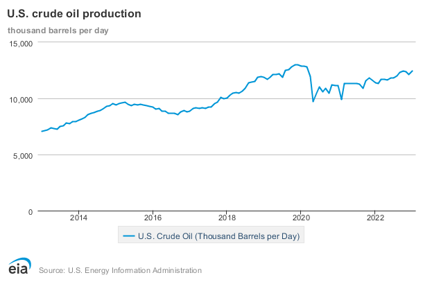
US oil production has been risen over the past years (before the unprecedented situation in 2020) and stayed at about 12.8 million barrels per day in December 2019. This represents an increase from 2008 to early 2015, decrease in production from around mid 2015 to September 2016, and then increase in production again from then to late 2019. Production from 2014 to 2018 has been over 8.0 million Bbl/d. In 2016, U.S. crude oil production represents only about 55% of consumption, with the remainder coming in the form of imports. However, as Figure 3 shows, imports continue to decline as domestic crude supplies increase.
The rise in domestic oil production is mostly attributed to the new, “unconventional”, sources found in shale formations and high levels of oil price make the production from these sources more profitable. Advances in seismology (“3-D”), directional drilling (“horizontal”) and, fracturing methods (“fracking”), have made this once inaccessible resource commonplace today. Contrary to some beliefs, the number one source of imported crude oil in the US is not the Middle East, but Canada. Oil from tar sands in their Western Provinces is shipped via pipeline into the US.
Figure 2 is extracted from the EIA report on the U.S. crude oil production [44]. Figure 2 shows the upward trend in oil production over the (6) years before 2015, downward trend from mid 2015 to late 2016, and upward production trend again from late 2016 to late 2019 (before the unprecedented global pandemic in 2020). (Based on the latest completed study by the Energy Information Agency of the US Department of Energy.) This link from the EIA includes the historical data from the 20th century [45].
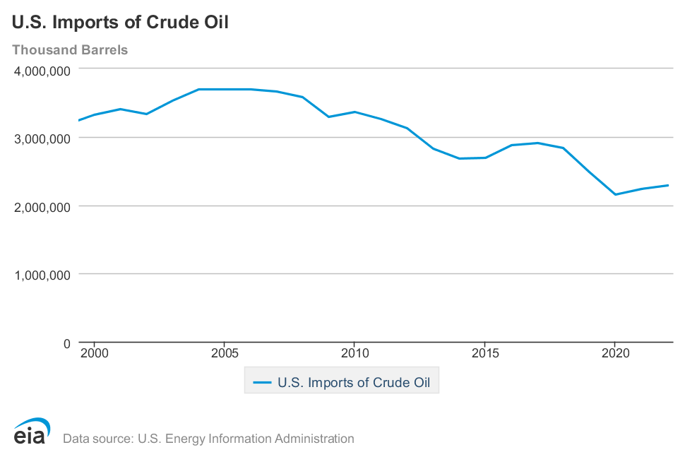
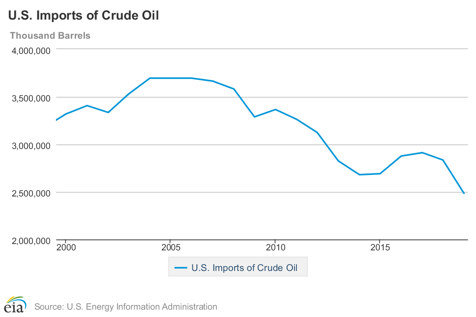
Figure 3 shows the downward trend in oil imports for the same time period (2000 - 2020).
Crude oil is produced in 32 states in the United States and as of 2021 about 71% of domestic crude oil production comes from the following five states [47]:
- Texas: 42.4%
- New Mexico: 11.1%
- North Dakota 9.9%
- Alaska: 3.9%
- Colorado: 3.7%
Crude oil is produced in about 100 countries around the world. In 2021 about half of the world oil production comes from the following five countries [47]:
- United States: 14.5%
- Russia: 13.1%
- Saudi Arabia: 12.1%
- Iraq: 5.3%
- Canada: 5.8%
Here are the top five oil consumer countries in the world in 2021 [48]:
- United States: 21%
- China: 15%
- India: 5%
- Russia: 4%
- Japan: 4%
According to EIA [49]:
" In 2022, the United States imported about 8.32 million barrels per day (b/d) of petroleum from 80 countries. Petroleum includes crude oil, hydrocarbon gas liquids (HGLs), refined petroleum products such as gasoline and diesel fuel, and biofuels. Crude oil imports of about 6.28 million b/d accounted for about 75% of U.S. total gross petroleum imports, and non-crude oil petroleum accounted for about 25% of U.S. total gross petroleum imports. ”
Here are the top five countries that the US is importing oil from with their share in 2022 [50]:
- Canada: 4.4 million barrels per day (52%)
- Mexico: 0.81 million barrels per day (10%)
- Saudi Arabia: 0.56 million barrels per day (7%)
- Iraq: 0.31 million barrels per day (4%)
- Columbia: 0.24 million barrels per day (3%)
Figure 4 displays the China and India oil production and consumption since the 90s. As you can see in this graph, oil consumption by these two countries has increased substantially during the past two decades, while their oil production hasn't changed significantly. This gap has created a large oil demand from these two counties in the global oil market.
Factors Influencing Crude Oil Price
Many, many factors can influence the price of crude oil either directly or indirectly. Some of the major factors influencing US crude oil prices are:
- US weather – mostly winter, as the demand for heating oil impacts crude oil prices. The Northeastern part of the US is the world's single largest consumer of heating oil.
- Geopolitical events - in any oil-producing region of the world where conflicts exist that could potentially interrupt supply.
- US dollar vs. foreign currencies - as mentioned previously, a devalued US dollar gives foreign investors more money to buy crude oil contracts and, vice versa, a stronger US dollar discourages foreign investment in crude oil contracts.
- US economy - strength or weakness directly impacts the perception of energy consumption. Several economic indicators are released weekly.
- World economy - as stated in the introduction, we are now in a truly global economy and what happens in one country can affect all others.
- Production & imports vs. demand - reports on domestic oil production & imports vs. consumption can cause prices to vary greatly. Some of the reports/statistics are listed below:
- Baker Hughes Drilling Report of active rigs - this oilfield service company keeps track of the total number of rigs actively drilling for oil and gas, and they report the statistics weekly. A rise in rigs means more potential supply coming-on down-the-road. A drop in the rig count could mean less supply down the road.
- West Texas Intermediate (WTI) crude vs. Brent North Sea crude - Brent crude oil is presently the global standard and trades in London. Its prices reflect demand in continental Europe, which can influence the price of imported crude here in the US.
- Weekly Crude Oil & Distillates Inventory Report (Energy Information Agency) - The Department of Energy releases a report every week that gives the current amount of crude oil and distillates in the nation's storage facilities. (Distillates include heating oil, diesel, gasoline, etc.) Increases in the inventory are viewed as an increase in supply, while decreases are seen as an indicator of increased demand. Another key piece of information presented is that of "refinery utilization". The higher the utilization percentage, the higher the demand for crude and vice versa.
- OPEC [31] - The Organization of the Petroleum Exporting Countries, OPEC, was formed in 1960 by the first five members including Iran, Iraq, Kuwait, Saudi Arabia, and Venezuela and has 14 members as of May 2017. OPEC members control about 73% of the world's total proved oil reserves and produced 44% of the world's total crude oil in 2016. OPEC has a significant impact on the oil market, managing the oil production, and oil price.
- Cross-commodity markets – as we will see in future lessons, most fuels, such as gasoline, diesel fuel, heating oil, and jet fuel, are all produced from crude oil. The demand shift for these commodities, such as travel season and weather change, will also impact the demand of crude oil. The EIA Weekly Crude Oil & Distillates Inventory Report also lists inventory changes for these commodities.
The following videos go into greater detail about the factors which can influence crude oil prices. Please note that some of the statistics might be a bit out of date, but please do not worry about that. These are just examples and are meant to teach you about how the various factors influence the market. You will not be responsible for the example details.
(The lecture notes can be found in the Lesson 2 module in Canvas (Lesson 2: Supply/Demand Fundamentals for Natural Gas & Crude Oil.)
Fundamental Factors Part 1: Weather and the US Economy
(9:04 minutes)
Farid Tayari: In this video and following videos, I'm going to explain the factors that are influencing the crude oil price. So there are many factors that can have an impact on crude oil price that we can name some of them as weather, US economy, international economy, US dollar exchange rate comparing to other foreign currencies, geopolitical events, supply and demand statistics, and crude oil and petroleum distillates inventory.
First, US weather-- heating oil is a refined distillate of crude oil. And it is being used by 5.7 million-- around 6 million households-- in the United States for space heating and warming of the water. Around 80% of those six million households are living in Northeast part of the country.
So if there is a cold winter, if there is a cold wave hitting this part of the country, we're expecting to have higher demand for heating oil. And it could be a good signal for price of oil being potentially increased.
I put a link here and this is slide to EIA website-- Energy Information Administration-- that includes the heating oil prices. So in addition to looking for data such as temperature or having a potential prediction of wind chill, there's also another indicator called HDD or Heating Degree Days. It's a good sign for energy demand.
So HDD represents the amount of energy being used to heat the space inside the building to reach 65 degrees, Fahrenheit. The lower outside temperature, it means that more energy has to be used for space heating. So historical and forecasted issues can be found at this link. It takes you to the National Oceanic and Atmospheric Administration. It can be a good metric for expected demand of heating oil and eventually, crude oil.
So one thing that we have to note that HDD is always positive-- there's no negative-- in case for the summer, the outside temperature is higher than 65, and then energy has to be used to cool down the space to the 65. We use this metric called CDD, or Cooling Degree Days. It's a measure for the amount of energy that needs to be used to cool down the building.
The other weather event that could potentially affect the crude oil price is a hurricane. According to EIA-- Energy Information Administration-- around 23% of the offshore oil production and 45% of the US oil refining capacity is around the Gulf of Mexico. And this is the section that in case of hurricane, that could potentially be affected and the supply can be interrupted.
So around 24 hours before the hurricane, the site-- which is a production site or drilling site-- has to be evacuated. And after the hurricane, it takes around at least 72 hours to reman the facility and start production.
In case of hurricane, there are two possible things that can happen, the interruption in the production because the site has to be evacuated. Or if the hurricane is severe, it can also damage the facility. For example, two cases-- Hurricane Katrina in 2005, 12 rigs and 30 platforms were damaged. And 18 of those platforms were completely destroyed.
Hurricane Ivan in 2004 damaged seven rigs and destroyed two rigs, and seven platforms destroyed. And it had consequences-- flooding and so on and so forth. And this can cause the supply interruption or the prediction of supply interruption. So when there is an interruption in supply, price can potentially increase.
I put a link here and it takes you to National Hurricane Center. It is a good resource for getting information of hurricane events. The official hurricane season begins on June 1st and it goes to November 3rd with a peak around mid-September. During this time, Weather Channel provides information through tropical update report.
The other factor that fixed the price of oil is the economy. Oil is a global commodity and the United States economy and other major countries in terms of economy. They can potentially influence the price of crude oil.
In this video, I'm going to explain the effect of US economy and crude oil. And in the following videos, I'm going to focus on international aspects of the economy and factors that are affecting crude oil price.
So energy runs the economy. And every aspect of economy can potentially influence the crude oil price. If economy is doing good, if economy is growing, it means there will be higher demand in future. Demand will be increasing. Strength and weakness of domestic economy directly impacts their prices, and also the perception of prices change and the prediction of the demand and eventually, the price predictions and the reaction of the traders to the price.
One of the most obvious and most frequently reported indications of economic health is stock market. Dow- Jones Industrial Index, S&P 500, and NASDAQ are daily reports that indicate the performance of the stock market. If these metrics are showing a good performance for the stock market, it means that economy is growing. And it could go up.
There are also weekly, monthly, quarterly economic reports that can have immediate impact on the price perception. Unemployment rate and reports being published by US Department of Labor-- this report is published every Friday. Institute of Supply Management Index report published monthly. Inflation rate, which is calculated from the CPI, Consumer Price Index, is being reported by US Bureau of Labor Statistics. It's a monthly report. GDP, US Gross Domestic Product, which also being published by Bureau of Economic Analysis and it's being published quarterly.
Also, US Department of Commerce's Economic and Statistics Administration has number of economic indicators that include data from US Census Bureau and US Bureau of Economic Analysis. These economic metrics are including construction spending, housing starts, housing sales, US international trade, monthly wholesale trade, manufacturing and trade, sales for retail and food services, personal income, and personal spending.
Also, quarterly earning reports from US companies-- these are the report metrics in economic parameters that can help us predict the future demand.
The next video-- so I'm going to explain the other factors that can influence crude oil price.
Fundamental Factors Part 2: International Economy, US Exchange Rate and Geopolitical Events
(9:29 minutes)
Farid Tayari: Following the previous videos, in this video, I'm going to continue explaining the factors that are affecting crude oil price. In this video, I will start with international economy. As we learned previously, crude oil is an international commodity. It's a global commodity. It's being traded everywhere in the world. Every part of the world economy can have impact on the crude oil price. Some countries that are contributing to biggest portion of crude oil consumption, their economy can potentially have a big impact on crude oil price.
So when trading starts early in the morning on the exchange in New York, Asian market is already closed and European market is at midday. So the behavior of the market, the signs of how market will behave, they are already known.
And probably the most watched nation these days outside of the US is China. China is contributing to around 15% of the world GDP. And China is, after the United States, the second-largest consumer of crude oil.
After China, Japan used to be the third-largest consumer of crude oil. After the Fukushima nuclear disaster, Japan's imports of fossil fuel increased. But at the moment, India is in the third place, taking Japan's place in oil consumption of the world. Also, the European Union and Europe region is consuming around 22% of world crude oil, and this data is from 2013.
So economic growth in these regions that are large consumers of crude oil can influence the crude oil. If the economy is doing good, if growth rate-- economic growth rate-- is high, it gives the signal that the demand in the future-- there will be high demand for crude oil in the future. And if the economy is slowing down, it means that the expected demand will not be as high as before. The increasing demand will be not as high as before, and it is going to potentially affect the price of crude oil.
The other factor that can potentially influence the crude oil price is the United States exchange rate. As you know, crude oil is globally being traded in US dollar. So the fluctuation of exchange rate, US dollar compared to other currencies, can potentially affect the crude oil price.
Why? Because there are many traders outside of the United States, and they are trading the crude oil which is being traded in US dollar. So if the dollar value decreases-- if US dollar loses its value-- it means that those traders living outside of the United States will have higher buying power. So they can buy more crude oil futures contracts. It means that there will be higher demand from outside of the United States. It will increase the demand of crude oil and can potentially increase the price.
So usually, there is a strong correlation, negative correlation, between the United States US dollar value and crude oil price. During the periods of a strong US dollar, foreign traders, investors try to sell their future contracts. And when the US dollar loses its value, they tend to buy more contracts.
The other factor that can impact the price of oil is geopolitical events, especially in the regions that are big producers of oil. Any conflict or potential conflict can impact the prices. Any news that can give the sense of potential interruption in supply can increase the price.
Please note that it doesn't necessarily need something to happen that interrupts the supply. Traders are also humans. They behave emotionally. They can react to the news in an emotional way. So if news says some potential conflicts in the region where large producing countries are located, it can potentially affect the perception of the supply in the future. It could potentially interrupt the supply, or it can influence the perception of the supply in the future and can have a significant impact on the crude oil prices.
For example, in mid-June 2014, WTI-- West Texas Intermediate-- crude oil price was about $107 per barrel. And at the end of that year, it went down to around $54 per barrel. We can explain this price behavior into two major factors that influence the price. First, the increased supplies of oil in the United States, mostly coming from unconventional reservoirs, shale and tight sands, because the price of oil was high. And at this price, at around $100, it's totally economically feasible to produce oil from costly unconventional reserves.
Around this time, Saudi Arabia-- that is, one of the largest producers and exporters of crude oil-- tried to maintain the market share by flooding the market with cheap oil, but this strategy caused excess supply and price to drop substantially. Low price of oil can have a large impact on oil-producing countries that are highly dependent on the revenue from oil. Also, in the United States, the companies who are working on the exploration and production section of oil, they will have to cut back on exploration and drilling activities, too, because they lose their revenue. And potentially, if the price is too low, they can potentially-- the small companies-- they can go bankrupt.
The other major player in the oil global market is OPEC, or the Organization of Petroleum Exporting Countries. OPEC was formed in 1960 by the first five members, including Iran, Iraq, Kuwait, Saudi Arabia, and Venezuela. And right now, at the moment, 2017, it has 14 members. OPEC produced around 43% of the world's total crude oil in 2015, and OPEC members control about 73% of the world's total crude oil reserves. So every decision that OPEC members-- every agreement or even the meetings that don't come to an agreement can potentially affect the price of crude oil.
For example, if OPEC members come to an agreement and they cut back to production, it can cause the supply-- the world's total supply-- to decrease and eventually cause price increase. And if in their meetings, let's say there's time and there's a conflict-- politics is always involved in the decisions. If there is a period that prices are going down and they cannot come into an agreement for cutting back the production, then it can potentially affect market prices and potentially cannot stop the price decrease.
Fundamental Factors Part 3: Supply & Demand Statistics
(3:45 minutes)
Farid Tayari: Following the previous videos, in this video, I'm going to explain the factors that can influence the crude oil price.
The last factor that I'm going to explain is supply and demand statistics. Any informational report that can give some information about the production or consumption of crude oil and, also, its distillates products can cause an impact, can cause a price change.
There are a variety of reports being published by governmental entities, both US and international, as well as industry associations. And these reports are good sources to predict the behavior of the crude oil price.
EIA, Energy Information Administration, from the US Department of Energy, issues a report on the status of country's inventory of crude oil, and its various distillates. This report is being published every Wednesday at 9:30 AM, and it has several pieces of key supply and demand statistics.
I'm going to explain some of the items that are included in this report. First, a refinery utilization, the percentage of total US refinery capacity that is running indicates both demand for crude oil as well as production of gasoline.
And, two, is an import report, both raw crude oil and refined products, such as gasoline. They are imported and volumes are compared to last year, which could be indicators of improving or worsening the balance.
The other part of the report includes commercial crude oil inventory. The change in inventory from one week to the next week has a profound impact on crude oil prices from a trading standpoint.
Analysts provide forecasts for the change in inventory ahead of the actual report. And financial and energy commodity traders react to the difference between the forecasted and actual report.
The other piece of information that is included in the report is gasoline inventories. Total gasoline products, as well as, breakdown between finished gasoline and blending products, gives a picture of supply and demand for gasoline. A decrease in total products could mean more demand for refinery feedstocks. Surplus could mean just opposite.
If there is an inventory, it means that there will be more supply to the market, and price won't go up, then they potentially could go down.
Information about distillate fuel is also included in EIA Inventory report which, in this category, is mainly about heating oil. And as I explained earlier, the cold winter-- the cold weather, or low temperature, means higher demand for heating oil.
And if there is low inventory, if there is low storage, it can be translated to low shortage of supply and higher prices in the cold days.
Optional Video: Exchange Rate Example
So as I explained in previous video, value of the US dollar or US dollar exchange rate versus foreign currencies is one of the factors that affects the crude oil price. As we know, crude oil is a global commodity that is traded globally, but in US dollars. So any fluctuations in the exchange rate between US dollar and foreign currencies can affect the crude oil price.
I'm going to explain that in a very simple example. Let's assume there are two traders who trade crude oil futures contracts. So one is Trader A is in the United States and Trader B is in Europe. Trader A has $1,000, and Trader B has 1,000 euros.
So first, let's assume that the exchange rate between US dollar and euro is 1-to-1 so meaning that $1 is equivalent to 1 euro. And let's assume that crude oil price is $50 per barrel. OK, let's see what happens for Trader A.
Trader A has $1,000 and can buy 20 barrels of crude oil or can buy futures contract equivalent to 20 barrels of crude oil. So $1,000 divided by 50 leaves 20 barrels of crude oil.
Let's see what happens to the trader in Europe. So Trader B has 1,000 euros. The first thing that Trader B has to do is going to the exchange and convert the 1,000 euros to the equivalent dollar amount, which is $1,000. Then with that amount, Trader B can buy crude oil. So Trader B can also buy 20 barrels of crude oil.
So the total demand will be 20 from inside the United States and 20 internationally, assuming there only two traders. So there will be 40 barrels of crude oil demand, total demand.
OK, now let's assume the case that US dollar loses its value. So again, same traders, two traders, Trader A is located in the United States and has $1,000. Trader B is in Europe and has 1,000 euros.
And now let's assume US dollar has lost its value. Now $1 is equivalent to 0.8 euros. Or with 1 euro, you can get $1.25. And let's assume the crude oil price has stayed the same, $50 per barrel. And let's see what happens.
OK, trader A still has $1,000. Crude oil price is still $50 per barrel. So Trader A inside the United States can still get that 20 barrels of crude oil.
And let's see what happens to Trader B. Trader B has 1,000 euros. Trader B has to go and exchange that 1,000 euros to equivalent dollar. And as we can see, because dollar has lost its value, that 1,000 euros will be converted to $1,250 because, with 1 euros, Trader B will get $1.25. So Trader B has $1,250, which can buy five more contracts. So Trader B would end up buying 25 barrels of crude oil or futures contract equivalent to 25 barrels of crude oil.
So 20 barrels demand from Trader A inside the United States and 25 barrels of crude oil demand from Trader B outside the United States-- so total demand will be 20 plus 25, 45 barrels. So we can see the demand increase from 40 barrels to 45 barrels when the dollar has lost its value. So it means that demand has increased. So demand curve shifted to the left-hand side, which changes the market equilibrium price for crude oil. And it potentially increases the crude oil price.
Natural Gas
Extracted natural gas [7] is mainly composed of methane, with small amounts of hydrocarbon gas liquids (HGL) and nonhydrocarbon gases. After natural gas is produced, it has to be processed and impurities have to be removed to meet the pipeline standards and become marketable. The infrastructure of natural gas delivery (before distribution) can be divided into three main categories [33]:
- Processing: removing and separating other hydrocarbons, contaminants, and impurities.
- Transportation: transporting the processed natural gas with the pipeline.
- Storage: storing natural gas in underground storage sites (depleted natural gas or oil fields, salt caverns, and aquifers) for high-demand periods.
In 2021, U.S. dry natural gas production was about 34.5 trillion cubic feet and about 13% more than total U.S. gas consumption. This year, five states produced about 69% of total U.S. dry natural gas:
- Texas: 24.6%
- Pennsylvania: 21.8%
- Louisiana: 9.9%
- West Virginia: 7.4%
- Oklahoma: 6.7%
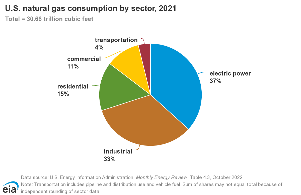
Natural gas is used in more than 50% of US homes for space heating and hot water. In addition, it is the largest source of energy for electrical generation at the moment (2021), see Figure 5. Natural Gas is also widely used in industrial, commercial, and industrial sectors. Figure 6 illustrates the breakdown of natural gas consumption by sector.
Click to expand to provide more information
| Energy source | Share of total |
|---|---|
| Natural gas | 38% |
| Coal | 23% |
| Nuclear | 20% |
| Renewables (total) | 17% |
| Hydropower | 6.6% |
| Wind | 7.3% |
| Solar | 1.8% |
| Biomass | 1.4% |
| Geothermal | 0.4% |
Click to expand to provide more information
| Energy Sector | Share of total |
|---|---|
| Electric Power | 36% |
| Industrial | 33% |
| Residential | 16% |
| Commercial | 11% |
| Transportation | 3% |
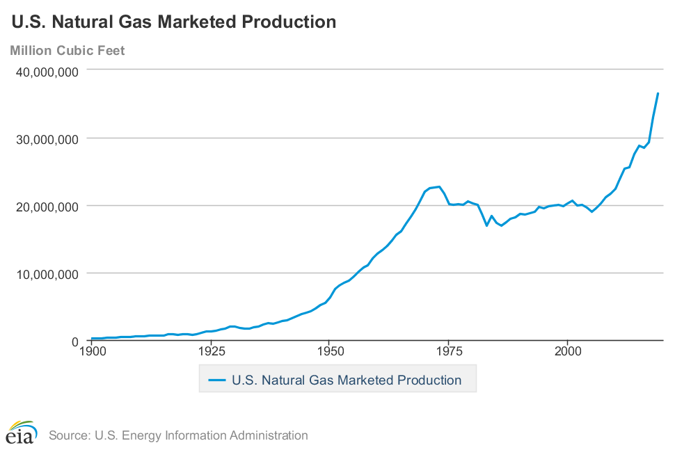
Domestic production in the US (see Figure 7) has grown dramatically in recent years due to the same advanced technologies that have allowed crude oil production to increase: “3-D” seismology, horizontal drilling and new “fracking” methods. All contribute to successful recoveries from hard formations such as the new “shales.”
Click for a text alternative to Figure 7
| Decade | Natural Gas Production |
|---|---|
| 1900 | 1028,000 |
| 1910 | 509,000 |
| 1920 | 812,000 |
| 1930 | 1,978,911 |
| 1940 | 2,733,819 |
| 1950 | 6,282,060 |
| 1960 | 12,771,038 |
| 1970 | 21,920,642 |
| 1980 | 20,179,724 |
| 1990 | 18,593,792 |
| 2000 | 20,197,511 |
| 2010 | 22,381,873 |
| 2019 | 36,515,188 |
Figure 8 illustrates the growth in the production of the currently active shale basins in the US. As you can see in the graph, natural gas production from Marcellus Shale formations, located mostly in Pennsylvania, West Virginia, Ohio, and New York, has been increasing during the past decade and has the largest portion of gas production among the shale formations.
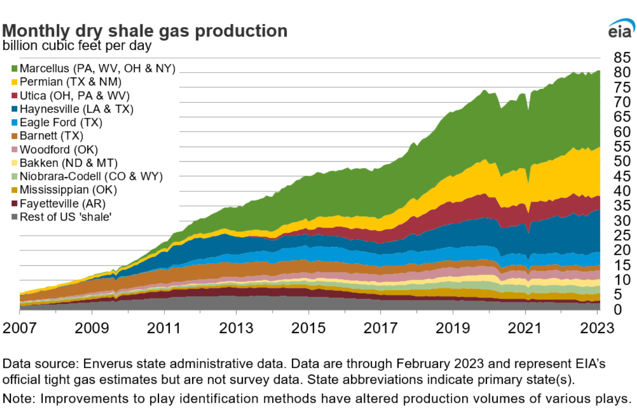
Production Growth of Active U.S. Shale Basins
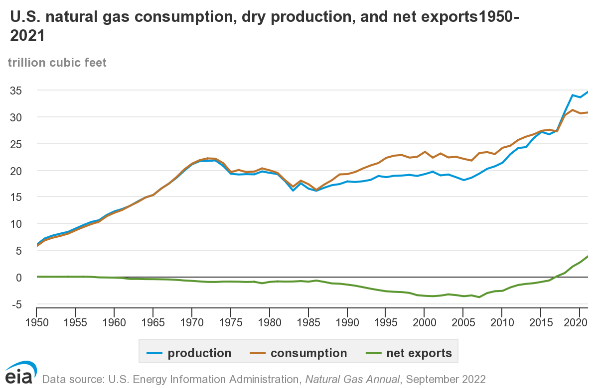
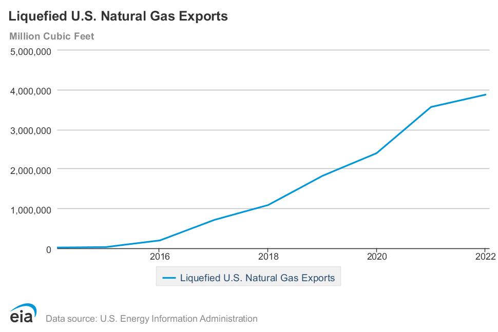
Due to the increasing demand since the late 1980s, the US also imports natural gas (see Figure 9). Canada represents the largest source (more than 97%) of imported natural gas, with Mexico contributing a minor amount. The export of natural gas had been very limited through pipeline export points into Canada and Mexico. However, the export changed dramatically since 2016 due to the skyrocketing LNG export. In 2017, the U.S. became a net exporter of natural gas and in 2021, the LNG export exceeded pipeline export for the first time since 1990.
Factors Influencing Natural Gas Price
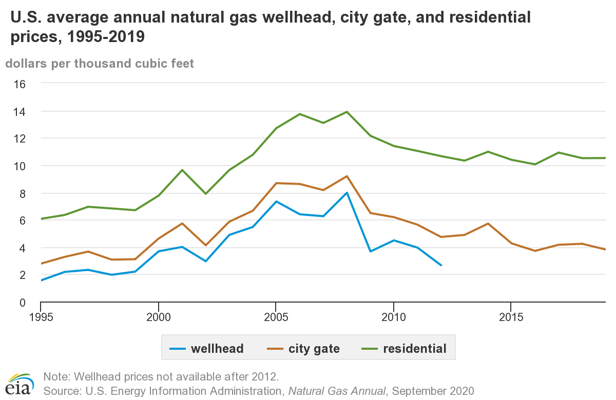
Figure 11 displays the U.S. average annual natural gas wellhead, city gate, and residential prices (1995-2019). Please note the increasing trend before 2008 and decreasing prices after. In order to fully understand these trends, have a look at Figure 7 (U.S. annual natural gas marketed production [53]) and U.S. GDP [56]from 1995-2019.
In contrast to crude oil, natural gas was almost strictly a domestic North American commodity* whose price is more influenced by weather and the health of the US economy. It is gradually becoming a global commodity in recent years due to increasing LNG export capacity [57]. Other factors, such as the level of US natural gas inventory, impact prices on a weekly basis. While US economic indicators, such as the stock market, employment figures, housing and, manufacturing indexes, are deemed to be indicative of demand for natural gas, global economies and the US dollar do not have much effect on pricing in this country.
Among the major factors influencing US natural gas prices are:
- Weather – over 50% of American homes are heated by natural gas; hot weather leads to more electrical generation for air-conditioning loads, and natural gas represents about 25% of that market. Hurricanes in the Gulf of Mexico disrupt supply as platforms are evacuated ahead of the storms, and the hurricanes can also damage the rigs.
- US economy - as with crude oil, fluctuations in the economy translate into an increase or, decrease, in energy consumption.
- Production levels vs. demand indicators - statistics showing flowing natural gas are compared with demand indicators to determine if the market is "short" or "long" supply. Here are some major indicators.
- Weekly Natural Gas Inventory Report (Energy Information Agency) - every Thursday morning, the US government releases data on the amount of natural gas that is in the nation's underground storage facilities. Injections and withdrawals from storage are also indicative of supply and demand dynamics.
- Baker Hughes Drilling Report of active rigs - the field services company reports weekly on the number of drilling rigs actively pursuing oil and/or natural gas. The change in number and type impact the perception of supply in the future.
- Electrical generation “fuel-switching” - besides the impact of overall demand for electricity, a large amount of the country's power plants that are fueled by coal can actually switch to natural gas, but only if prices are competitive. Also, the Nuclear Regulatory Agency publishes a daily status report for all nuclear plants in the US. When plants are down, more electricity is generated by natural gas.
- Global demand – US LNG reaches most regions of the world [58]. Major economies such as Brazil, China, France, India, Japan, Netherlands are purchasing more and more US LNG. The price of LNG is higher than natural gas exported by pipeline due to costs associated with compression, transportation, and decompression. However, it is still profitable given the increasing worldwide demand for clean energy.
The following video goes into greater detail about the factors which can influence natural gas prices. (The lecture notes can be found in module 2 in Canvas. (Lesson 2: Supply/Demand Fundamentals for Natural Gas & Crude Oil.)
As we explore pricing for crude oil and natural gas in a later lesson, we will consider the major influential factors for each and define their individual impact. We will also have a weekly activity about the market prices for crude oil and natural gas and the factors we believe affect them.
Note: When commodity price is expected to go up, the market is called bullish [59]. In this case, an investor will invest in the commodity. On the other hand, if prices are expected to go down, then it’s called a bearish [59] market. In this situation, an investor is expecting the commodity to lose its value. Consequently, the investor sells the financial commodity.
PRESENTER: In this video, I'm going to explain the factors that can influence natural gas price. In contrast to crude oil, natural gas is almost not a global commodity, yet. It can be construed as a domestic commodity in the United States. So things that are happening outside the United States, they don't have a major impact on the natural gas prices.
So we can focus on the factors that are happening in the United States. And two of these major factors are the US economy and weather events. Other factors, such as the level of US natural gas inventory, can also impact the natural gas prices on a weekly basis.
The higher natural gas inventory means high supply or having enough supply for fluctuations in demand. So if there is a high level of inventory, it can translate to not having, not experiencing, not expecting the higher price of natural gas.
US economic indicators such as the stock market, employment, figures housing and manufacturing, they impact the natural gas prices. On the other side, global economy, US dollar exchange rate would not have an impact on the pricing of natural gas.
The first factor is the weather. More than 50% of American homes are heated by natural gas. So any cold or extreme weather could potentially increase the price if there is a shortage of supply. If there is an unexpected demand, it could shift the price to higher prices.
Also, hot weather could cause the price increase, because people will use air conditioning to lower the inside temperature for space cooling. And so increase in demand for electricity could potentially increase the natural gas prices.
The other weather event is hurricanes, same as crude oil, that we explain how a hurricane in the region of Gulf of Mexico can disrupt the supply and damage platforms. Evacuation and recovery after a hurricane can potentially interrupt the supply.
US economy-- similar to crude oil, fluctuations in economy translate into an increase or decrease in energy consumption. North American natural gas is not a truly global commodity, so the global economy does not have an impact on the price of natural gas.
The other factor that could potentially affect the natural gas price is the reports about production levels versus demand indicators. Any statistics, any information about supply or demand of natural gas can potentially affect the price.
EIA, Energy Information Administration from Department of Energy, publishes a weekly report every Thursday at 9:30 AM. This report is about natural gas storage. And it has some pieces of information that I'm going to explain them in the following slides.
So EIA Weekly Natural Gas Storage Report includes pieces of information on natural gas storage. The first piece of information is regional breakdown-- the activity for the EIA-defined regions, which includes the major consuming regions, both east and west, and producing region. The producing region is further broken down into the salt and non-salt storage facilities, with the majority of the salt caverns existing along the Gulf Coast.
Injections, or gas added, and withdrawals, gas removed, by region can be telling about the weather conditions in each area. A good balance is when the consuming regions are withdrawing the same amount of gas as producing region is injecting gas.
The other very important piece of information included in EIA Weekly Natural Gas Storage Report is the total gas in storage. It is the change in historic levels from one week to the next week. It is the first thing that traders and other parties involved in the natural gas market would look to for guidance.
Excess storage, a high level of storage or injection in the report, can be translated to a bearish price signal. That is, the production exceeds demand for the prior week.
The converse is also true for the removal of gas from the storage, or withdrawal in the report, that can indicate demand exceeded the production for the prior week. Prior to the release of the report, analysts have compiled forecasts in the variance of the actual volume to these predictions.
The other piece of information that can be found in EIA Weekly Natural Gas Storage Report is a comparison to a year ago. This data includes the information-- the current inventory level compared to the same period the previous year. In order to truly interpret this comparison correctly, we must consider the weather in this year with the last year, if there was or there is harsh winter we are experiencing or we were experiencing cold days.
The last piece of information in EIA Weekly Natural Gas Report that is important for us is a comparison to the five-year average that can be found in the report.
The other factor that can influence natural gas price is electrical generation fuel switching. A large amount of country's power plants were fueled by coal. And they can switch. They can switch their fuel to natural gas if natural gas prices are competitive or more restrictions are being enforced for the emissions. But this effect is a more long-term effect.
Also, the Nuclear Regulatory Agency publishes a daily status report for all nuclear power plants in the United States. When plants are down, more electricity is generated by natural gas.
Summary and Final Tasks
Key Learning Points: Lesson 2
- In 2008, the record run-up in oil prices actually represented a dynamic shift in the composition of market participants.
- Crude oil is a globally-traded commodity in a world where the economies of most countries are tightly intertwined.
- The US is gradually increasing its domestic oil production, thus reducing its crude imports.
- Natural gas is strictly a domestically traded commodity (until late 2015/early 2016 when we start to export LNG).
- Vast new reserves of natural gas have been found in “shale” plays due to new technological advances in exploration, drilling, completion, and production.
- The US is both an importer and exporter of natural gas.
- Several factors influence the prices of crude oil and natural gas.
Now that we have examined production and consumption in the United States as well as the energy “mix,” we will focus on the fuel sources that comprise over 57% of the energy used in this country. Crude oil, with refined products, and natural gas and related natural gas liquids (NGLs) make-up this large sector.
Reminder - Complete all of the Lesson 2 tasks!
You have reached the end of Lesson 2. Double-check the list of requirements on the first page of this lesson to make sure you have completed all of the activities listed there before beginning the next lesson.
Lesson 3 - The New York Mercantile Exchange (NYMEX) & Energy Contracts
Lesson 3 Introduction
Overview
In 2008, the price of crude oil on the New York Mercantile Exchange (NYMEX) hit an all-time high of $147 per barrel. And, within (6) months, the price had fallen to about $35. Again, in 2014, oil was over $100/Bbl in June only to fall to below $50/Bbl by December. While many factors led to these "peaks and troughs, the nature of futures trading and the exchange itself made this possible. The New York Mercantile Exchange has been around since the late 1800s. Financial energy commodity contracts, such as futures contracts, are traded on the New York Mercantile Exchange, and it is still the most influential financial energy commodities exchange in the world. Futures contracts are financial tools to hedge against the price fluctuations. In this lesson, we will explore the history of the exchange, how it functions, who participates, what commodities are traded and futures contracts. In this lesson, we will also learn about the NYMEX order flow. Standardized Order Forms are used on the floor of the NYMEX during order execution. All orders placed on the NYMEX to buy or sell contracts are done in a very precise manner where each party involved is fully aware of the details of the transaction.
Learning Outcomes
At the successful completion of this lesson, students should be able to:
- explain the history and development of the exchange;
- identify the components of a standard NYMEX contract and which commodities are traded;
- list the specific contract specifications for:
- natural gas,
- crude oil,
- heating oil,
- unleaded gasoline;
- describe the importance of the “price discovery” function provided by the exchange of energy commodities;
- know the difference between “pit” and electronic trading;
- recognize various exchange “floor” personnel and players;
- explain NYMEX - order execution & electronic trading:
- list the order flow from the physical customer through the exchange,
- recognize that very few contracts ever actually get delivered physically,
- explain the electronic trading and "high-frequency trading" for futures contracts;
- identify information about the futures market including risks, functions, regulators, margins, motions, price, short and long positions;
- explain the concept of the “zero-sum” game in financial contracts;
- recognize and research the various factors impacting supply and demand for natural gas and crude oil for this week, and assess their potential impact on market pricing for each factor.
What is due for Lesson 3?
This lesson will take us one week to complete. The following items will be due Sunday at 11:59 p.m. Eastern Time.
- Quiz
- Lesson 3 activities as assigned in Canvas
Questions?
If you have any questions, please post them to our General Course Questions discussion forum (not email), located under Modules in Canvas. The TA and I will check that discussion forum daily to respond. While you are there, feel free to post your own responses if you, too, are able to help out a classmate.
Reading & Viewing Assignments: Lesson 3
Reading Assignment:
- Seng - Chapters 3, 4, 5
- Errera & Brown - Chapter 2, "Market Mechanics" in preparation for this week's quizzes.
- "A Brief Review of the History of Futures [60]”. You can find this article in Canvas Module Lesson 3.
Optional Materials
Please take some time to review the optional materials. They will give you context for the rest of the lesson.
Optional Readings
Investopedia Article and Video
What are Futures Video (20:30 minutes)
The New York Mercantile Exchange
Financial energy commodity contracts are traded on the New York Mercantile Exchange (NYMEX). The New York Mercantile Exchange building is located on the Hudson River in New York City and owned and operated by CME Group of Chicago (Chicago Mercantile Exchange & Chicago Board of Trade). NYMEX has offices in other cities as well (Boston, Washington, Atlanta, San Francisco, Dubai, London, and Tokyo.) The New York Mercantile Exchange [63] started in the 1800s. There were scattered markets for the goods in large cities. You can picture a city like New York City and agricultural products being brought in and sold in various parts of it. So, some entrepreneurial businessmen decided that they needed a central exchange. So, in 1872, it was founded as the Butter and Cheese Exchange. In 1880, it was changed to the Butter, Cheese, and Egg Exchange. And then, finally, in 1882, it was changed to its present name, the New York Mercantile Exchange.
Later products would include yellow globe onions, apples, potatoes, plywood, and platinum. Platinum is the only one of these products which is still traded today on the New York Mercantile Exchange. Today, it trades crude oil, heating oil, gasoline, propane, natural gas, platinum, and palladium.
For a quick overview of the Exchange, view this "This is NYMEX" video (2:20 minutes).
[MUSIC PLAYING]
PRESENTER: New York City, financial capital of the world. Home to global giants in banking, investing, and finance.
AUDIENCE: We only have four and 1/2.
AUDIENCE: Sell 20 and 1/2.
PRESENTER: Where there is always a transaction on the table, money on the line, and business never sleeps. It's also home to the New York Mercantile Exchange where billions of dollars in commodities are traded every day, but one way or another, impact business and consumer alike.
[MUSIC PLAYING]
[CALLS AT MERCANTILE EXCHANGE]
PRESENTER: What appears, at first glance, to be pure pandemonium, is in reality, a very structured business, as highly choreographed and orchestrated as any Broadway show. The New York Mercantile Exchange is a marketplace for buying and selling futures and options contracts in commodities. For instance, energy products such as crude oil, natural gas, gasoline, home heating oil, propane, and electricity, as well as metals like gold, silver, copper, aluminum, and platinum.
But what does that matter to me, you might ask. Here's an example. Oil refiners sell fuel-- mainly gasoline, heating oil, diesel, and jet fuel. Airlines buy large quantities of jet fuel. It's similar to heating oil, and the two products are often priced within a few cents of each other. As price protection against unexpected increases in the cost of jet fuel, an airline can buy a heating oil futures contract at today's known price for use in the future.
If prices rise tomorrow, the airline saves money by having locked in a lower fuel cost. That's called hedging. The fuel savings could mean lower airfares for you and me. The same principle applies to heating oil we use to keep our homes warm in winter, and the gasoline we buy for our cars. When companies protect themselves from volatile prices, they can help pass along those savings to their customers.
Price transparency is a key advantage to doing business on the Exchange. Everyone knows the price of all contracts being bought or sold. This benefits the entire marketplace and builds confidence and credibility for business and consumer alike.
90 bid!
Futures Contracts and NYMEX
Futures contract
Forward and Futures Contracts Crude Oil (11:02)
okay let's start reviewing what are the futures and before that I will need to explain forward what contracts first. So, forward contracts, let's say on the left-hand side we have an oil producing company on the left on the right hand side we have a refinery which consumes oil and produces some refined products. So, on the left hand side we have producer that sells the oil on the right hand side we have consumers that buys the oil. So, let's say right now the refinery needs some crude oil the producer has some oil. They just sell and buy and that's it. Okay, but this is an ongoing business activity, right? The producer knows that for anytime future they know the production rate and they know how much crude oil they will have in the future. Also refinery this is a continuous production process, they know they're going to need a crude oil for almost any time in the future, right? Both of these are concerned about market fluctuations and also they want to make sure they market for crude for the produced crude oil or they can have the crude oil that they need. And also they're concerned about the price. The producer is concerned that, okay what if price drops, we're going to lose money. On the other side the refinery is concerned that if price goes up we're going to lose money and they want to hedge their risk against price fluctuations. So what we can what they can do is, they can negotiate a contract which is called forward and they can discuss three things: time, price and quantity. And let's say we are going to sign a contract that sometime in the future, let's say in November, at the locked price of 50 dollars the producer is going to deliver some specific quantity of crude oil let's say 5000 barrels to the refinery. So, they have a contract that locks the price for delivery in some time in the future and they can have many of these. So, this is called forward contract. And by doing that they first make sure the producer has a market for crude oil, the consumer they know for sure they will have crude oil in November. Also, they know the price is locked. The price is locked. They lock the price 50 dollars. The price doesn't change. Okay what are the kind of them restriction, limitations, of these forward contracts?
Okay first let's say these two entities, the producers and consumers, they're not exactly the same size. Let's say the refinery is a very large, or the producer is very large producer, one of them is a lot smaller or larger than the other one. So, then, they have to go and probably find 10 other counterparties to find, negotiate, and sign the contract for each of them and they have to do it for almost every month, soon and so forth. It's doable, it is still uh an ongoing activity in the financial market, but it's not the most efficient way of doing it.
The other problem with this is, let's say this contract is signed to deliver the crude oil in November and the price is locked at 50 dollars. Let's say, a couple of months to the November, let's say price of crude oil goes up. Let's say it goes to sixty dollars. So, if it goes in the market it's sixty dollars, but under this contract it is locked at fifty dollars. So, because it is locked, then, the producer loses money. Because, if there was no contract producer could have sold it in the market at sixty dollars. So, the producer will get more and more upset that, okay, I am losing money under this contract, but there is no way that they can cancel the contract. On the other side, if price of crude oil starts going down, the producer is happy but the consumer cannot uh cancel the contract and go and buy the cheaper oil in the market. They have to pay the 50 dollars for locked price. So the problem is they cannot cancel the contract at all.
So, this is the kind of the introduction how there is a better more efficient type of contract needed based on the forward and that's going to be called futures, which I’m going to explain in in a bit.
Okay, now let's make some changes and move toward that more efficient contract which we'll call it later on futures. Okay, the first thing that we want to do is, we want to introduce the third party here. And let's say, we call this third party, and say instead of producer going and trying to find consumers, these producers will just go and sign a contract with this third party, call it exchange or call it a businessman, businesswoman, a company. And the consumer, the refinery, will also go and signs the contract with this third party. So, it solves the problem that they don't need to go and find, let's say 10 more, consumers and sign individual contracts for them.
Let's make some little more adjustments. Let's say we make these contracts standard. You remember in the previous slide I said look at these contracts, these forward contracts are case based? they are signed for the specific case and between these companies and their contract terms are negotiated between these two entities?
Now let's introduce a type of contract that is, all the terms are standard, there's nothing negotiable. These are all fixed in place and nobody can change them. The quantity is fixed, the delivery point is fixed, the price is fixed, which I’m going to talk about the price in a bit. And everything is fixed under these contracts, except the delivery date. And delivery date goes by the incremental month. It's either January or February or March, so on. The only difference between these contracts is the delivery date or expiration date. So, when we make these contracts exactly similar, there's no need for any negotiation back and forth. So, we will have these standard contracts and what we can do is we can have all the other entities to join this market and trade these contracts.
So, what will end up with an exchange in the middle, which will have these contracts, they are all standard, exactly the same. And we have these players that the actual producer the refinery and the oil producing can also join as one of these players in the market. So, they can either buy these contracts or they can sell them. If they buy this contract, we call them their position is long. If they sell this contract their position is short.
If they buy the contract, long position, they have to take the delivered crude oil, they will receive the crude oil when contract expires. On the other side, those players, those entities who sold the contract, their position is short. They have to deliver the crude oil, the amount of crude oil at the expiration date.
Because, these all these contracts are exactly the same, these are called futures. They have the fixed quantity, one thousand barrels of crude oil, the delivery point is fixed, Cushing Oklahoma and the spec is WTI, West Texas Intermediate and that's low sulfur, sweet, crude oil and the expiration day goes by the month, January, February, March and so on. The price is set by these trades by these market movements, sell and buy, supply and demand. If somebody does not like the loss that they are making, based on the price movement, they can get out of the contract anytime they want. They don't have to wait until the expiration date. If the prices are going up and the position is short, they can just immediately close the position by buying back, buy closing the position with the exchange.
The entities who are long these contracts, the entities who bought the contracts, will make money, will profit, when price goes up. On the other side, if an entity has a short position, will lose money. If price starts to go down, long position will lose money and short position will make money.
Okay, an important point here, these contracts are binding. The entity, the party that is short, the part that sold this contract, has to deliver crude oil at the expiration date. If that party is not an oil producing company, or if that party is not interested in delivering or cannot deliver the crude oil, they have to close their position, they have to cancel the contract. How? if they are short, they have to buy back; if they are long, they have to sell.
The definition given by the New York Mercantile Exchange is “...a legally binding obligation for the holder of the contract to buy or sell a particular commodity at a specific price and location at a specific date in the future.” The key word here is future. These are known as futures. We are buying and selling energy commodities at a future date and time. And again, this is a legally binding obligation. This is what makes exchanges a sound place to conduct business. If you fail to perform under a contractual obligation with the New York Mercantile Exchange, there are both financial and legal ramifications.
The components of a standard NYMEX energy contract are as follows.
- the name of the commodity and exact specifications of the commodity (for example WTI crude oil, natural gas, heating oil, unleaded gasoline;
- the quantity and volume of the commodity (for example 1,000 barrels for the crude oil futures contract);
- the price, is determined by the market and is normally what we are most interested in;
- the location that the commodity has to be delivered;
- and then the date, the date that the commodity has to be delivered. At what future point in time do we wish to buy or sell the energy commodity?
Here are the links to the crude oil [64]and natural gas [65] features in NYMEX. These links take you to the crude oil futures quotes [66] and natural gas futures quotes [67]in NYMEX. You can click on the “About This Report” at the bottom right of the table to find the column head explanations. Reported information in the table will be explained later in this lesson.
The trades on the New York Mercantile Exchange between the counterparties are conducted under the International Swaps and Derivatives Association, or ISDA, 2002 Master Agreement. This is a standardized contract under which all financial energy commodity contracts are traded.
Functions of Energy Contracts
Price Discovery
One of the primary functions of energy contracts on the New York Mercantile Exchange is that they provide us price discovery. We can establish a price for crude oil, natural gas, heating oil, and unleaded gasoline at any future point in time. Years back, prior to the advent of the New York Mercantile Exchange, no one could really tell what the price was at any point in time. Most trades were conducted over the telephone. But now, with the New York Mercantile Exchange, at any point in time, you can look up the live trading.
The New York Mercantile Exchange is owned by the Chicago Mercantile Exchange, or the CME Group. If you go to cmegroup.com [68], you can find the commodity prices. Under the "Trading" tab, you can find the commodity and then the commodity futures contract.
Hedging
In addition, this allows us to perform what we call hedging. Hedging is to reduce risk in a transaction. In the case of the futures contracts, it helps us to reduce our price and/or physical risk. We may be concerned about high prices if we're a consumer of energy commodities. We may be concerned about low prices if we are a producer of energy commodities. We may also be concerned about receiving physical supply or having to guarantee physical market. The New York Mercantile Exchange contracts guarantee that.
Futures Market Characteristics
Remember from microeconomics [69]that a perfectly competitive market has the following characteristics: 1) Nobody has market power 2) Product is homogeneous 3) Information is perfect and 4) There is no barrier to enter and exit. Indeed, such a hypothetical market with all these characteristics doesn’t exist in the real world. However, the futures market is one of the closest markets to the perfect competition. There are many buyers and sellers. There is no or very limited government intervention in this market. There is no significant barrier to enter and exit the market, except the legal and financial responsibility of market participants. Traded products are futures contracts that are standard and homogenous for each commodity. In addition to these, cost of information is relatively low. All these features make the futures market an efficient market. And from microeconomics, we know that in an efficient market 1) price is determined by the market dynamics, 2) price represents the true value of the good, and 3) price fluctuates around the true value of the good. These happen because the futures market is highly related to the cash market. A portion (even though it’s a very small portion) of the futures contracts ends in actual delivery.
Note that an important feature of the futures contracts is, gains and losses to each party is settled every day. This is called marking to market or daily settlement. It’s equivalent to closing the contract each day and opening another one for the next day. When opening the position, either long or short, each party only pays a small amount of money, which called margin requirement. The margin is used for daily gain or loss (daily settlements) due to the price changes. And if the loss is more than amount in the margin account, the party has to immediately deposit more money into the account.
The following lecture will take you through the history of the NYMEX, the type of trading that occurs ("pit" vs. electronic), the major players, the commodities traded, and futures contract specifications.
NYMEX Contract Lecture
Figure 1 displays the NYMEX building located on the Hudson River in New York City and the NYMEX trading floor, where all the trades occur. Watch the video lecture at the bottom of this page to learn more about the NYMEX futures contracts.
Key Learning Points for the Mini-Lecture: NYMEX Contracts
While watching the Mini-Lecture, keep in mind the following key points and questions:
- NYMEX contracts are legally binding obligations to buy or sell commodities.
- Contracts are standardized.
- Each commodity contract has volume, price, location, and date.
- The NYMEX trades 5 energy commodities along with 2 precious metals.
- Trading occurs both in the “pits” of the Exchange, as well as electronically.
- Margin requirements discourage many from "speculative" trading.
- The Exchange has a unique set of symbols to identify the commodity/month/year.
- All prices are quoted in US dollars and cents.
- Each commodity has a specific delivery point.
- West Texas Intermediate Crude (WTI) is the standard traded on the NYMEX.
- Futures contracts provide “price discovery.”
- Market participants include “commercial” or those interested in the physical commodity, and “non-commercial,” or “speculators.”
The following video lecture is 20:30 minutes long.
Some of the common terms used by NYMEX. An ask-- an ask is a motion to sell at a specific price. It's the same as an offer. So ask and offer are interchangeable. It's your asking price. What do you wish to get in the marketplace for your commodity? And notice this is a motion because they're addressing the idea of the physical trading that takes place in the pits, the movement of hand gestures back and forth as traders buy and sell. A bid, then, is the opposite. It's a motion to buy at a specific price. What is your bid for the energy commodity?
A bull-- in this case, we're talking about a person. It's one who anticipates prices will increase or volatility in the market will increase. They're the opposite of a bear. A bear is one who anticipates a decline in price or the volatility in the marketplace. Obviously, the opposite of a bull.
This is a picture of the New York Mercantile Exchange trading floor. It just so happens in the foreground is the natural gas trading pit. Off to the left, barely seen, is the crude oil trading pit. Notice the various colors of jackets around the floor. I will identify who some of those are in a minute. But the yellow jackets, for the most part, those are NYMEX compliance personnel. The multi-colored jackets, the blues, the burgundies, some of the other colors, represent brokers, what are known as clearing brokers on the floor of the New York Mercantile Exchange. They have posted credit, and they have licenses to trade on behalf of their clients.
So we have the floor brokers, which I mentioned. We have locals. These are the individuals and firms and in some cases funds that have a large amount of money and wish to trade. They are speculators. They're not interested in the physical commodities whatsoever. They're interested in price movement, and wherever the price is moving, that's where they want to be.
Ring reporters and ring chairmen-- we'll drop back here a second, and I will show you. The ring reporters are in the yellow jackets near the trading rings themselves. There is a podium, if you can tell, situated above the natural gas pit with some personnel in yellow jackets. Those are the ring chairmen. Their primary responsibility is to oversee the activity of the pits and to resolve any disputes. Since we have people who are yelling orders back and forth to one another and using paper slips, sometimes mistakes can be made, and if there's a disagreement over the actual details of a trade, the ring chairman is supposed to step down and resolve that trade between the two counterparties.
We have floor committee members. Those are basically NYMEX committee members. The New York Mercantile Exchange also has compliance people. And the Commodity Futures Trading Commission is the regulatory body for energy financial derivative trading. They have their own personnel on the floor as well. And then there are hundreds of line staff from the New York Mercantile Exchange.
We'll now talk about each one of the specific contracts for energy commodities. The first is crude oil. The symbol is CL. We refer to this as West Texas Intermediate, or WTI crude. It is low sulfur, and so, therefore, is given the nickname sweet crude. The NYMEX contract for crude oil was initiated in 1983. Every contract represents 1,000 barrels, which is the equivalent of 42,000 gallons of oil. Price quotes on the New York Mercantile Exchange are all US dollars and cents, in this case per barrel. A minimum price fluctuation-- that is, the amount that the price has to move for a trade to take place-- is a penny, or $10 a barrel.
The delivery point for crude oil under this contract is what's known as FOB, or free on board, or delivered to the seller's facilities at Cushing, Oklahoma and to any pipeline or storage facility with access to Cushing Storage, TEPPCO, or Equilon pipelines. So if you buy or sell crude oil contracts on NYMEX for a particular month, you are obligated to either receive the crude oil or deliver the crude oil at Cushing, Oklahoma.
Deliveries are to be made uniformly across the month. This is the contractual obligation. The idea here is to make all parties deliver as equally as possible. The actual obligation-- for instance, if I sold 30 contracts for the month of September, that means 30,000 barrels of crude oil-- the Exchange would like me to deliver that at 1,000 barrels a day. However, if I cannot, my real legal obligation is 30,000 barrels for the month.
The trading hours on NYMEX for what we consider to be the open outcry or pit trading, the general session where the traders are in the pits yelling orders back to one another, run from 9:00 AM to 2:30 PM Eastern Standard Time. The Chicago Mercantile Exchange also has an electronic trading platform known as Globex, and this is virtually 24 hours a day, seven days a week. It starts at 6:00 PM on Sunday evenings and ends at 5:45 PM on Friday, Eastern Time.
Crude oil can be traded for up to nine years. And then we also have products that are known as strips. These are available for terms of 2 to 30 consecutive months. In essence, strips amount to an average price. If I wanted to buy six months' worth of crude, rather than go out and have my broker quote me one month's price at a time, they'll just give me an average price across the six months. Therefore, I am purchasing a six-month strip of crude oil.
The last trading day, every contract expires. Again, we are talking about future contracts. So currently, the closest future contract is September. The crude oil contract, then, settles three business days prior to the 25th of the month. So just in case the 25th is a non-trading day, either a weekend day or a holiday, the settlement occurs three business days prior to the business day that is prior to the business day ahead of the 25th. I know that sounds very confusing. I can't quite figure it out myself half the time.
Margin requirements. This is a big issue here. You can see that if you want to buy or sell crude oil contracts, for every single contract that you wish to enter into, you have to have $5,100 in a margin account. That's a safety net against losses that you could incur. This protects your clearing broker and protects the New York Mercantile Exchange from default by you as a counterparty.
This also discourages a lot of traders from just jumping in and trying to trade contracts. For example, if a trader wanted to speculate on 10 crude oil contracts-- that's only 10,000 barrels-- that's not a lot of volume, per se. They would have to put $51,000 in a margin account before they could even get started.
Here is the symbol breakdown. When you look at futures screens, or if you see the prices reported in the Wall Street Journal or any other type of publication, you'll see these funny symbols. The first two letters of the symbol represent the energy commodity themselves. So CL represents crude oil. The second letter is the actual month of delivery. For example, U equals September. The final symbol is the number that corresponds to the year. In our example, 2. So the September 2012 contract for crude oil on the NYMEX is expressed as CLU2.
Other symbols that represent energy commodities-- NG for natural gas, HO for heating oil. RBOB represents unleaded gasoline, and then PN for propane. And then here's the breakdown of the symbols that they use. Feel free to use this as a cheat sheet if you ever run across those quotes and can't remember what they mean.
When you look at futures screens, you're going to see column headers that will use these types of terms. When you see the open, that's the opening price at the opening bell. When you see people on television ringing the bell for the open of whatever market it might be-- the stock market, the NYMEX, the Chicago Mercantile Exchange-- as soon as the bell goes off, the very first trade that is consummated, that price is registered as the open for the day.
The high is the highest price that traded that day, including the after-hours electronic trading. The low is the lowest price that traded for that day, including after-hours electronic trading. That gives us the range on the day-- what was the entire range of pricing that day.
When you see last, that's the last trade that just occurred. In other words, what was the last trade that had occurred? The net would be the change in price from that last trade to the one prior to it. So are we going up or are we going down as we're trading currently? And then change-- the change is the change in price from the trade that just occurred, from that last trade, versus the prior day's settlement. What was the final price for the energy commodity the day before, and where do we sit relative to that today? That's what change represents.
We refer to futures contract trading as a zero-sum game. For every buyer, there is a seller. I can't buy crude oil contracts without someone being willing to sell them to me, nor can I sell them without a market. And believe it or not, less than 2% of all the contracts traded actually go to physical delivery. In other words, less than 2% of the contracts will actually be energy commodities exchanged between counterparties. Now, on the one hand, that may sound like a small number, but with each crude oil contract representing 1,000 barrels, and you can trade between 50,000 and 100,000 contracts a day, it does amount to a substantial amount of physical energy commodities being exchanged.
This is what a typical futures screen would look like. These are the headers that I mentioned to you. On the day that I printed this off, you can see the last trade was $92.68 and, represented a drop of $0.19 from the prior day's settle of $92.87 in the far right corner there. We had the opening price of $93.25, and a high and low on the day as well. And the very far right column is the time at which the trade occurred.
Natural gas futures contracts. The contract unit is 10,000 MMBtus-- that is, 10,000 million British thermal units. Prices are quoted in US dollars and cents, and the minimum fluctuation between trades has to be 1/10 of a penny or what we refer to as a tick. Trading hours are exactly the same, but the trading months for natural gas-- you can actually trade natural gas out 12 years if there was, in fact, a need to buy or sell for that long of a period of time.
Last trading day for natural gas contracts, the futures, is the third business day prior to the first calendar day of the delivery month. We do trade options in energy futures contracts. In the case of natural gas, those expire one day prior to the actual contract itself.
The delivery point for buying and selling under NYMEX natural gas contracts is a place known as the Henry Hub in Erath, Louisiana. Texaco has their Henry plant in Erath, Louisiana. Sabine Pipeline Company runs the hub on behalf of the New York Mercantile Exchange. And again, the delivery period is to be uniform across the month of production for which the contracts were exchanged.
This is a schematic of the pipelines going in and out of the Henry Hub. There are various sources of natural gas coming offshore, onshore. There is gas moving to the Northeast, the Southeast, the Upper Midwest, as well as from Louisiana back into Texas. So it made an ideal market hub for indicating various supply and demand.
Settlement price. Every day, the New York Mercantile Exchange will put together a final price for that day's trading. The settlement price is the weighted average of all the trades that occur during the last two minutes of trading in that regular session. Now, when the closest future month, or what we call the prompt month, when that contract expires, they're going to take the total number of trades in the last 30 minutes to come up with a weighted average, and that will be the price for that month. And that month rolls off, as we say, and it's in the history books.
Margin requirements for natural gas are substantially less than crude oil, but the value is substantially less, so there's only $2,100 margin requirement per contract.
This is what a natural gas futures screen would look like. If you ever see one of these on a trading floor or somewhere else, perhaps on someone's screen who trades in these contracts, this is what it would look like.
We're now going to talk about unleaded gasoline, referred to as RBOB. RBOB stands for Reformulated Blend for Oxygenated Blending. What we get at the gas pump-- you usually have the opportunity to get 100% unleaded in very few places. Mostly, it's a 90/10-- that is, it's 90% gasoline, 10% ethanol or some other type of blending component. In some cases, you hear about E85, which is 85% unleaded, 15% of some other additive, normally something like ethanol.
So what's traded on the New York Mercantile Exchange is actually the 100% unleaded. It becomes a feedstock for unleaded because it's only 90% of what we get at the pump unless we're buying 100% unleaded. So it's reformulated blend for oxygenated blending. They're going to blend oxygenators into the unleaded gasoline.
The oxygenators are seasonal in nature, depending on the regions. Again, oxygenators help to burn the gasoline more efficiently and therefore reduce the emissions. Oxygenators are things such as ethane, ethanol, butane, isobutane, and natural gasolines.
Every RBOB contract is 42,000 gallons. US dollars and cents, and the minimum fluctuation is 1/1000 of a penny per gallon. The delivery point is free onboard or delivered into the petroleum products terminals in New York Harbor. Margin requirements-- $8,100 per contract.
Last but not least, heating oil, or HO. It's sometimes referred to as number two fuel oil. Every contract is 42,000 gallons. We are still dealing with US dollars and cents per barrel. Minimum price fluctuation is 1/1000 of a penny per gallon. The delivery point is the same as for RBOB, and that is free onboard or delivered to the petroleum products terminals in New York Harbor. Everything else pretty much remains the same under the standardized NYMEX contracts.
NOTE:
The lecture notes can be found in the Lesson 3 module in Canvas (Lesson 3: The New York Mercantile Exchange (NYMEX) & Energy Contracts.)
Optional Material
Trading Pit Hand Signals
As explained in the video, “ask” is a motion to sell and “bid” is a motion to buy at a specific price. We use the word motion because the traders use hand signals to communicate to one another across the pits. The following video illustrates some of these hand signals. Please watch the 3:37 minute video, Trading Pit Hand Signals [72] below.
Click for a transcript.
Many of Chicago’s “open outcry” trading pits are closing this month. This form of trading was born in Chicago, centered around traders shouting orders to brokers. Eventually, it got so loud a sign language developed in the pits.
PRESENTER 1: If you've ever seen Ferris Bueller's Day Off, when he's up there and they're making all those signs, this was a way for traders to communicate with other traders, with other brokers, with other order fillers.
PRESENTER 2: It's loud, crazy on the floor, and you need to communicate very simply.
PRESENTER 3: There's so much noise that if I said "buy 20" or whatever, they can't hear. So, I have to have some type of a symbol that shows.
PRESENTER 4: Let me get a sight line to a guy. And I'll say, buy 10 (pointer finger pointed at forehead and then quickly moved away from head). And then this guy will tell the broker, buy 10.
So we'll have a guy standing next to the broker. We'll have a guy on the phone. The customer will tell me what he wants to do, and I'll have it flashed in (using a hand signal for buy 10) -- way faster. And it cuts out all the nonsense.
PRESENTER 1: If you wanted to say, buy 100 S&Ps at the market, you would go, buy 100 (fist on forehead). And you'd go like this with your hand (slash hand in front of you, palm down), and that would mean market.
PRESENTER 2: If you're buying, you have your palms in, just like you're grabbing something toward you. If you're selling, you're pushing something away.
PRESENTER 4: We were in the S&P, so they had dimes and nickels. So it was 10 bid (pointer finger up, palm toward you), 15 bid (pointer finger bent at knuckle, palm toward you), 20 bid (pointer and middle fingers up, palm toward you), quarter bid (pointer and middle fingers bent at knuckle, palm toward you), 30 bid-- I'm sorry, 30 bid (pinky, ring and middle fingers up, palm towards you), 35 bid (pinky, ring and middle fingers bent at knuckles, palm towards you), half (all 5 fingers up, facing towards you), doubles (all five fingers bend at knuckles, facing towards you) -- even money (fist pointing towards you).
PRESENTER 5: It could be one (pointer finger up pointing away from you). I mean, naturally, you go right up to one. Or it could be five (all five fingers up pointing away from you), or you could do this, 10 (both hands facing out with all fingers up). This could be 100 (fist on forehead facing out and pushing away from your head).
PRESENTER 3: Now, you're usually holding your deck in the other hand. Your pencil may be in this hand, so you're giving your symbols. But you have your deck or your card, your trading cards, in this hand.
So you don't have two hands to go six or seven. So what we would do is turn a hand sideways. So now this becomes six (pointer finger pointing to the right, palm towards you), seven (pointer and middle fingers pointing to the right, palm towards you), eight (pinky, ring and middle fingers pointing to the right, palm towards you), nine (four fingers pointing to the right, palms towards you).
PRESENTER 2: And then as you go up to 10 (right-hand pointer finger touching forehead), 20 (right hand pointer and middle fingers touching forehead), 30 (right hand pinky, ring and middle finger touching forehead), 40 (right hand four fingers touching forehead), 50 (right hand palm open touching forehead) --
PRESENTER 1: 60 (left-hand pointer finger touching forehead), 70 (left-hand pointer and middle fingers touching forehead), 80 (left-hand pinky, ring, and middle finger touching forehead), 90 (left hand four fingers touching forehead), and 100 (left fist touching forehead).
PRESENTER 3: And later when the big trades came in and the options and the Eurodollars, they even came out with 1,000, which was the crossed hands (fists) in front of your chest.
PRESENTER 2: And then you really want to make a statement on the trading floor, you're going 1,000 (arms crossed in front of you, left with fist, right with pointer finger out), 2,000 (arms crossed in front of you, left with fist, right with pointer and middle fingers out), 3,000 (arms crossed in front of you, left with fist, right with pinky, pointer and middle fingers out).
PRESENTER 4: It's way faster and way easier to do. And you can put orders into different areas, too. You could look at a guy to the right of you. If he wasn't paying attention, maybe the guy next to you would. So create a competition, too, amongst brokers and clerks.
PRESENTER 2: One ear is listening to the marketplace. The other part of your brain is having a conversation, and you're not missing a cue. That's amazing to me.
So I thought this would be just really a good life skill to have. You're in the grocery store. Instead of yelling the amount-- hey, just get five, just five-- no, it doesn't work.
PRESENTER 4: You're out (wave a hand in front of your neck a few times). That was another good one.
PRESENTER 1: Or he'll go like this to a bartender. I need three more beers.
PRESENTER 4: Right.
PRESENTER 5: Or out.
PRESENTER 1: Out.
PRESENTER 5: Out.
[INTERPOSING VOICES]
PRESENTER 1: Cut off. I'm cut off.
PRESENTER 4: [LAUGHING] Right.
PRESENTER 3: Yeah, I always thought that was quite ridiculous. I see these guys going to the bar and says, yeah, cost me $20. I'm thinking you got to-- the same guys that used to go into the bar with their trading jackets on. [LAUGHING] I mean, I always thought that was a little hokey. But no, I never did use the hand signals.
MAN 1: 186.9 halves.
MAN 2: Two dollars. Three or four, all you want.
MAN 3: Cut!
PRESENTER 5: I would try most of the time not to even use the hand signal.
NYMEX Order Flow
All orders placed on the NYMEX to buy or sell contracts are done in a very precise manner with each party involved fully aware of the details of the transaction. As legally-binding agreements, non-performance under a futures contract can have severe financial and legal consequences. Therefore, most phone conversations are taped to ensure the accuracy of the orders placed as well as the results of the execution of those orders. Standardized order forms are used during order execution and daily "check-outs" occur between brokers and their clients for verification of all trades conducted that day. In this section, we will follow a natural gas futures contract trade from the beginning to end for a producer and end-user wishing to lock-in a fixed price for a 12-month period.
Key Learning Points for the Mini-Lecture: NYMEX Order Flow
While watching the mini-lecture, keep in mind the following key points and questions:
- All orders must be placed with a “clearing” broker who guarantees the trades.
- Contracts can be used for pure trading or “hedging” physical and price risks.
- Energy Trading companies & Financial Brokers provide risk services to their customers.
- Orders flow from customer’s representative through the financial trading process.
- Orders with NYMEX can be filled via the traditional “pit” trading or electronic platforms.
- Less than 2% of all contracts traded ever become physical transactions.
- Trading is a “zero-sum” game. For every winner, there is a loser (there are two sides to every trade).
NYMEX Order Flow Lecture
The following video is 10:40 minutes long.
As mentioned in the introduction to this lecture, we're going to walk through the specific steps of executing a buy and sell order on the floor of the New York Mercantile Exchange. We're going to be doing this during the regular session where there are active traders in the pits doing what they call the open outcry trading. In order to understand what's going on, there are two key terms here that we're going to need to understand.
One is a bid. And it's a motion to buy a futures contract at a specified price. The opposite of that is an offer. Again, a motion to sell a futures contract at a specific price. And that's also known as the asking price. And we use the word motion because the traders are using various hand signals to communicate to one another across the pits, if they're buyers or sellers, what volume, and what price.
So the example we're going to use in this case is a 12-month price, a 12-month "strip" average of $3.50. As mentioned in Lesson Seven, you can go out and you can buy or sell contracts at an average price as opposed to having to buy or sell at each individual month's price. In this case, we're looking at 12 months out. So currently, this 12-month strip is running $3.50. And there's a producer out there who would like to lock this price in, or better, if he or she can get that. So the producer's going to call a trader at the energy company and tell them that they're interested.
So the trader will turn around then and they'll ask the personnel on the fixed price desk to call New York and find out where the market currently is, where are the bids, where are the offers, for this 12- month strip for natural gas. Energy trading companies that have financial derivative trading, they will have a fixed price desk. These are the personnel mostly responsible for dealing with the New York Mercantile Exchange.
So the fixed price desk calls their broker on the floor of the New York Mercantile Exchange to find out the current market quotes and both the bid and offers. Now the person that they're talking to is the clearing broker and, specifically, the phone clerk. If you recall the picture of the floor of the Mercantile Exchange from Lesson Seven, you can picture those phone banks. So this is where that phone call is going to.
The fixed price desk person turns around then and gives the trader the current market quote. The producer then gets that bid and offer from the trader. And given that the market is still in the $3.50 range, the producer decides that he or she would like to lock in the price of $3.50 or better for the next 12 months if in fact it can be executed. The trader now takes the order from the producer and passes it along to the fixed price desk.
Now, at this point in time, the producer is obligated to perform under this contract. In other words, the producer realizes that the energy trading company's going to have to enter into the legally binding contracts on the New York Mercantile Exchange to obtain this fixed price for them. So the producer is going to have to perform by giving the physical gas when the time comes to the energy trading company.
So, the trader gives that order, the sell order, to the fixed price desk. The fixed price desk then calls New York again and, tells the phone clerk with the clearing broker on the floor of the NYMEX that they would like to sell the one month strip $3.50. The phone clerk immediately stamps the ticket that they have, indicating when the order was received from the fixed price desk at the energy trading company.
The phone clerk will then walk over to the pits and hand a copy of that ticket to their broker who is trading in the pits themselves. That pit broker then offers out the 12-month strip into the market at $3.50. Another broker, who has received a buy order from another customer, decides to go ahead and lift the offer on the 12-month strip at $3.50. So keep in mind that, as we mentioned in the prior lesson, it's a zero-sum game. For every buyer, there is a seller.
So, in this case, the producer is having the trading company sell contracts for them. There has to be a buyer across the pit willing to buy those contracts in order for the deal to be consummated. So in this case, there happened to be an interested party on the other hand. And for our purposes, we'll go ahead and assume that it's an end user who's interested in buying the natural gas at $3.50 for the next 12 months.
So, once the counterparty across the pit has gone ahead and lifted the order, the broker now hands the order back to their phone clerk. And the pit brokers also then have an official form that they have to fill out for the New York Mercantile Exchange, which includes the details of the transaction. So the phone clerk now time stamps the ticket, as in they've had it timestamped when the order was received, and it again is stamped with the time when the order is actually filled.
So, phone clerk calls the trader's fixed price desk. The trader's fixed price desk receives the fill from the floor of the NYMEX and repeats the fill verbally to ensure that there's no error. So the clearing broker phone clerk and the trading company's fixed price desk repeat the details of the transaction so that there's no mistake as to exactly what has occurred. And as mentioned in the prior lesson, the phones are also recorded.
So, if there's any dispute at the end of the day when it comes to checking out the trades between the energy trading company and their broker, they can pull the tapes, as we say, if there's a discrepancy and have it resolved that way. OK. The fixed price desk, now having confirmed the order, passes along the fill to the trader. The trader now passes along the completed order to the producer.
So, the producer has gotten done what the producer wanted. So the producer is now what we call hedged if natural gas prices decline below $3.50 over the next 12 months. So they can't get a price any lower than $3.50. However, because of that, they give up any upside. In other words, the producer you cannot get a price higher if the market does move up. But in this situation, the producer liked $3.50. And they wanted to make sure that prices didn't fall on them.
Here are some more terms that are frequently used in terms of New York Mercantile Exchange trading. We already covered the ask and the bid. A bull, a lot of you have already heard this term. But it's actually someone. It's a person who anticipates an increase in price or an increase in volatility. (Volatility is a measure in the magnitude of price change, as well as the frequency of the change in price). And they are the opposite of a bear. A bear, again, is a person who anticipates a decline in price or volatility. And they are the opposite of a bull.
Backwardation. It's a market situation in which the futures prices are lower in each succeeding delivery. It's also known as an inverted market. It's the opposite of contango. So let's take, for instance, the September crude oil contract. If right now it was the highest price, and October was lower than September, and November was lower than October, and so forth, we would have a backward- dated market. Because the normal situation is, the prompt month or near month, and for several months going out, prices do rise.
A broker. A broker is a party or company which is paid a fee for transactions in the financial and physical markets. Brokers do not take title to the contracts. They do not take title to the commodity being traded. They simply join counterparties together and they extract a fee for doing so. They are truly middlemen. The cash market is the market for a cash commodity where the actual physical product is traded.
So, we've mentioned a couple of times, we differentiate between financial and physical or cash marketplaces. When I talked about the pricing publications, they cover the cash market. The CFTC, that's the Commodity Futures Trading Commission. This is the federal agency responsible for the oversight of all commodities trading, not just energy commodities. The contango market. This is the opposite of the backward dated market. It's a market situation which the prices are higher in succeeding delivery months than in the prompt month.
To cover. We use that term to talk about a trader or company who happens to be short futures or options positions. In other words, they've sold contracts in anticipation of prices falling. And so that open position is known as a short position until such time as they buy those contracts back and cover that open position. A derivative is a financial instrument derived from a cash market commodity, a futures contract, or other financial instruments.
The New York Mercantile Exchange contract for natural gas is derived from natural gas itself, the commodity. And the same applies to the other energy commodities on the NYMEX. The last trading day. It's the last day of trading for the prompt month contract. Currently, for natural gas, it's three working days prior to the next calendar month. We covered the deadlines for each of these in Lesson seven.
Long. This is a market position based on owning contracts which must be sold, or the delivery of the underlying commodity must be accepted. It's the opposite of short. So a trader or a company who takes a long position, they're buying contracts in anticipation of prices rising. And then they will sell those contracts hopefully at a profit. The offer, we mentioned already. We talked about what an offer is.
Open outcry is the name given to the pit trading. OK. For NYMEX purposes, it's a method of public auction for making verbal bids and offers for contracts in the trading pits or trading rings of commodity exchanges. It is totally different than electronic trading platforms. The short. This is a market position based on selling contracts which must be brought back or the delivery of the underlying commodity must be made. It is the opposite of long.
So again, this is where traders are selling contracts in anticipation of prices falling. They'll buy them back and make a profit. We mentioned earlier the idea that when they are short, they'll have to cover those positions by buying the contracts back. Strike price. We will get more into this when we talk about options. But it's the price at which the underlying futures contract is bought or sold in the event that an option is exercised. It's also called an exercise price.
Optional Materials
High-Frequency Trading
"High Frequency Traders" (HFT) are impacting the market in a huge way by using super-computers to execute high volumes in nano-seconds. To get an explanation of HFT and their impact on the market, view this video (2:29 minutes).
SPEAKER 1: The problem with high-frequency trading is this. First of all, it's a myth that it hurts the common trader. Somebody that's on E-Trade and wants to buy IBM or some other trade isn't buying it for the nanosecond. They're not worried about that microsecond that they might have gotten and one-hundredth of a penny difference.
If you're an average trader, and you're worried about one-hundredth of a penny, you shouldn't be trading because you can't compete with the big boys. It's just not going to happen. So, most people-- public-- they trade. They buy something. They hold.
And they're looking for a few points or a long-term investment. So, the high-frequency traders really, I agree-- that don't affect them. Where the high-frequency traders affect everybody, and this is where you have what they call the flash crash. And I didn't really look at it as a flash crash.
I looked at it as that it was a vacuum, and some people say it's the same thing. Well, it's really not. When we were in the pit and news would come out, and all of a sudden want to be like 60 bid at 60, at 40, at 20, at even-- there'll be some person like me saying, OK, I'm 95 bid, and they go sold. There'll be another person that'll go 90. Then it will be sold.
And if somebody would come out 85 bid, it will be sold. So, there will be natural stops in the market. Natural volume because with 200 people in the pit, you have 200 different opinions. And everybody either had an opinion-- either it was too sold or too bought.
And the market would have ebb and flow going back and forth. Put in high-frequency trading. They tend to run on the same algorithm program. And when news comes out, they just pull.
SPEAKER 2: Pull out, panic the market drops. Yeah, and that's a real risk.
SPEAKER 1: They can pull out orders in nanoseconds. I can't tell you how many times that news came out, and a broker with 60 bid for 100. And before his clerk could grab him on his neck, I could go sold. OK, you can't do that now with the speed.
And what happens now is that it would be the equivalent of all the locals in the pit, the minute news came out that they would say, we're going to lunch. Have a nice time and see you later. And then the brokers would look.
And I've seen a broker's face when there's no bid when he has to sell something or no offer when he has to buy something. And that's why these vacuums now are just extraordinary. And that is the problem with where the high-frequency trader comes in. No, for 99% of the time, it's actually pretty good that they're there because they're arguing.
They are going back and forth with bids and offers, and I can get into any trade now. You can get into any trader now. Getting out's the problem.
Future of the Trading Floor
Please watch the following short video (1:55) about the future of the NYMEX trading floor and how electronic trading is affecting the trading pits.
PRESENTER: Even if you've never been to the famed trading pits, chances are, you know what they look like and sound like.
[VIDEO PLAYBACK]
[CROWD ROARING]
- Sell 30 April at 142!
[VIDEO PLAYBACK]
PRESENTER: Featured in films like Trading Places and Ferris Bueller's Day Off, the trading pits at the Chicago Mercantile Exchange were loud and hectic.
[VIDEO PLAYBACK]
[CROWD ROARING]
[END PLAYBACK]
PRESENTER: On July 6th, the futures pit in Chicago and New York, where buying and selling sets the prices for commodities like gold, wheat, and corn, roars one last time. The 167-year-old tradition of open outcry futures operations ends after the closing bell on Monday.
VIRGINIA MCGATHEY: For example, if I'm trying to buy 25 at 4 and a quarter, I would be saying that and also doing the hand signals at the same time. And then the opposite person would be saying, OK, I'm selling you 25 at 4 and quarter. And so, then we'd understand that I was buying and they were selling.
PRESENTER: Virginia McGathey, a grain trader on the Chicago Mercantile Exchange floor, just finished her last shift in the pit. In short, blame the computers. CME Group, which operates the trading pits in New York and Chicago, is shifting to electronic dealing. And CME Group held off on going all digital, even as rivals in New York and London embraced electronic trading.
VIRGINIA MCGATHEY: It's really heartbreaking on a particular level that it's ending this way. And I think, in talking with some of the other traders, the fact that we can't leave a legacy to children and grandchildren, that this is the end of the road-- it's just definitely not the same on a computer, not at all.
PRESENTER: And not all the pits are closing. One exception is the S&P 500 futures market, which remains open on the Chicago trading floor. In another sign of changing times, fans of CME Group can track the company on several social media sites, including Twitter, Facebook, Instagram, and Pinterest.
Summary and Final Tasks
Key Learning Points: Lesson 3
- The New York Mercantile Exchange is a market for crude oil, natural gas, heating oil, unleaded gasoline blend-stock, propane, platinum, and palladium.
- Futures are legally binding obligations that require delivering or receiving the commodity.
- Each contract lists commodity/price/date/location.
- The most important function of the Exchange is “price discovery” and transparency.
- Each commodity has its own delivery hub.
- WTI is the standard crude stream for futures contracts in crude oil.
- Only licensed brokers can trade on the Exchange.
- Trades have to be conducted with Clearing Brokers.
- There are two classes of market participants, “commercial,” or those interested in the physical commodity, and “non-commercial,” or “speculators.” Commercial entities use the contracts to "hedge" their price and market risk.
- Most trading is purely for financial gain, as only a small number of contractual obligations are fulfilled in the physical (cash) markets.
Now that we are familiar with the workings of the Exchange and futures contracts, we will walk through the cash market and its relationship to the financial market in the next lesson.
Reminder - Complete all of the Lesson 3 tasks!
You have reached the end of Lesson 3. Double-check the list of requirements on the first page of this lesson to make sure you have completed all of the activities listed there before beginning the next lesson.
Lesson 4 - Cash Market Pricing Methodologies & Publications
Lesson 4 Introduction
Overview
Energy is being consumed at every hour of the day everywhere on earth. Thus, energy commodities are being bought and sold constantly to fill this demand. When we are talking about prices for the actual physical production and consumption of natural gas and crude oil, we are talking about the "cash" market. In this lesson, we will explore the ways in which cash prices are established in the physical marketplace, historical pricing, the main publications that report these prices, and the methodologies they use to collect the data.
Learning Outcomes
At the successful completion of this lesson, students should be able to:
- identify key historical events of the natural gas “cash” market pricing, including price trends;
- outline the methodology for cash price determination;
- identify the relationship between futures and spot market prices;
- describe the relationship between futures contracts expiring in different months;
- explain the arbitrage and the situations in which arbitrage can be utilized;
- locate and summarize the key industry pricing publications and their uses:
- Platt's Inside FERC,
- Platt's Gas Daily,
- OPIS & ARGUS Price Reports for NGLs and Crude Oil.
What is due for this lesson?
This lesson will take us one week to complete. The following items will be due Sunday, 11:59 p.m. Eastern Time.
- Lesson 4 Quiz
- Lesson 4 activities as assigned in Canvas
Questions?
If you have any questions, please post them to our General Course Questions discussion forum (not email), located under Modules in Canvas. The TA and I will check that discussion forum daily to respond. While you are there, feel free to post your own responses if you, too, are able to help out a classmate.
Reading Assignment: Lesson 4
Reading Assignment:
- Seng - Chapter 2
- Errera & Brown - Chapter 3 in preparation for this week's quiz
This text is available to registered students via the Penn State Library. [73]
Introduction to the Spot Market
Spot market
The market where the actual physical commodity is traded is called the spot market. It can also be called the physical market or the cash market. This is similar to the traditional type of market that physical commodities are delivered for immediate sale and use on the spot. There are many local places where the spot market and local spot market price is determined by the local supply and local demand. Consequently, there might be high spot prices at one location and low spot prices at the other location, depending on the local supply and demand.
The actual demand for the physical energy commodity can change over time. In earlier lessons, we learned some of the factors that can affect the demand, for example cold winter days or hot summer days. However, local supply has to be planned by the producers in advance and since producers don’t know the exact demand ahead of time, spot market prices can become very volatile.
Relationship between futures and spot market prices
Basis represents the difference in price between financial and physical markets. Locational Basis is the difference in value between the financial commodity contract delivery point and other cash points.
The relationship between futures and spot market prices can be explained by parallelism and convergence. These two form the basics of hedging and speculation. The effectiveness of hedging is highly dependent on this relationship.
Parallelism explains the close relationship (high positive correlation) between futures and spot market prices. It basically says futures and spot market prices follow each other (vary together) closely, (with a gap or difference that is called basis). Parallelism recognizes the fact that both financial and physical markets are influenced by similar things.
Close to the expiration date, the futures contract price tends to get very close (converge) to the cash market price. It is called convergence. This happens because they can be substituted, meaning that a futures contract close to its expiration date is similar to having an immediate delivery of the commodity in the cash market.
If the futures price is higher than spot, the futures contract is sold at a “premium” to cash. The converse is true when the spot price is higher and the futures contract is sold at a “discount” to cash, this happens when demand in the spot market is higher than the supply and the spot prices go up.
Relationship between futures contracts that expire in different months
As explained in the previous lesson, futures contracts expiring in the later month tend to have higher prices, meaning that the closer expiry month usually has a lower price. This is called contango market.
Contango market represents sufficient supply of the commodity in the spot market to meet the demand. In a contango market, contracts with a later expiration date are sold at a “premium” to closer contracts, and close to expiry futures contracts are also sold at a premium to the cash. The “premium” is because of the carrying charges. For example, let’s assume a consumer needs the commodity in three months. The consumer has two alternatives: 1) buy the futures contracts that expire in three months, or 2) buy the commodity in the cash market now and store it for three months.
There are some costs associated with the second alternative (buying the commodity in the cash market and storing it until it is needed). These costs are called carrying charges (carrying costs) and mainly include storage cost, insurance, and cost of borrowed money to finance the commodity.
Because futures contracts don’t require carrying charges, futures contracts with later expiration dates tend to be traded at higher prices. This is the reason that we usually experience a contango market.
There are also situations where the market experiences the inverted behavior. In such situations, futures market that are expiring in later months are traded at lower prices compared to the ones that are expiring in earlier months. This is called “backwardation” or an “inverted market”. This could happen when there is a supply shortage in the cash market. In that case, spot market prices would be higher than the futures market.
Arbitrage
Arbitrage is buying the commodity at low price in one market and selling it at higher price in the other market and taking advantage of the price differences and making profit. Arbitrage causes the difference in prices to eventually decrease by balancing the supply in the two markets.
Locational arbitrage opportunity exists in the spot market as low risk. Spot market is spread out geographically and when the price difference in two locations is higher than the costs (mainly transportation cost) it’s a good opportunity for arbitrage.
As explained earlier, futures prices tend to be higher than spot prices and if the basis (price difference between futures and spot market) is higher than the carrying charges, arbitrage opportunity exists between futures and spot market. This arbitrage opportunity causes the convergence.
Natural Gas & Crude Oil - Physical Pricing
Even though the prices of energy "futures" influence the physical markets, prices are negotiated outside the infamous and chaotic trade floors of the exchanges. Buyers and sellers, looking at their supply and demand situations, make pricing decisions daily and actually buy and sell the physical commodities. The results of these trades are reported in industry publications and become market indicators for the physical "cash" market.
Key Learning Points for the Mini-Lecture: Physical Natural Gas & Crude Oil Pricing
While watching the mini-lecture, keep in mind the following key points and questions:
- Historically, prices were set for long-term contracts at fixed numbers.
- Deregulation created the need for shorter-term pricing.
- The physical commodity market has its own pricing scheme.
- Cash market prices are reported by industry publications using survey methodology and are known as “indexes” or “postings.”
- Inside FERC and Gas Daily are the main postings for natural gas.
- OPIS (Oil Producers Information Service) and ARGUS are the primary reports showing postings for crude oil & natural gas liquids (NGLs).
- Parallelism recognizes the fact that both financial and physical markets are influenced by similar things.
- Convergence is the tendency for the financial contract to approach the value of the physical commodity as it approaches settlement.
NOTE:
The lecture slides can be found in the Modules under Lesson 4: Energy Commodity Logistics - Crude Oil.
Now watch this 6:24 minute video about the cash pricing for the physical pricing of crude oil and natural gas.
In a previous lesson, we talked about the financial markets for crude oil and natural gas. And keep in mind, those are future markets. They're telling us what the prices are every day for months going forward. But what about what's happening each day? And what about the trading for the actual physical commodity where the financial markets aren't even involved?
We're going to talk about how those things are priced. And we're going to talk about some key publications that come out that actually show the results of all the trading in the physical marketplace. And then, the market uses those as price discovery. We talked about the fact before that the New York Mercantile Exchange provides price discovery for future months for crude oil and natural gas.
In terms of the natural gas industry itself, actually, both industries were heavily regulated over the years. And we've seen deregulation occur across the board in several industries-- the airline industry used to be regulated. The banking industry was regulated. The telecommunications industry was regulated.
And so, both crude oil and natural gas had been regulated. From the natural gas standpoint, the utilities and the pipelines were regulated. And then, from the crude oil standpoint, the pipeline industry itself was regulated. The idea in both those cases was to basically make sure there wasn't a monopoly, that no one had excessive market power that would hurt the market participants, especially the consumers.
So, generally speaking, way back, there were long-term contracts entered into, mostly by producers and pipelines for natural gas or utilities. These prices were fixed prices. That means they agreed upon a fixed price for the duration of that contract. Now, back in 1978, the Carter administration enacted what's known as the Natural Gas Policy Act. There was concern-- in fact, the Department of Energy back then predicted that the United States would run out of natural gas by the year 2000. Obviously, that was not the case.
But what they did was, they set prices for natural gas. They had a starting price. And then, every month, the price would go up by a few cents per MCF. Now, obviously, this was not market responsive. In other words, if you were producing, you were guaranteed a price, and you were guaranteed that price will go up every month. So, this is what led to the bubble that we had in the early '80s, and then the subsequent crash in natural gas pricing as producers decided just to go out and drill and produce as much as they could at these fixed prices. And the pipelines and utilities had to take the gas because they had these long-term commitments.
Finally, in January of 1985, those price controls of the NGPA had expired. This began what we call the beginning of the spot market. In other words, you would have these long-term arrangements where pipelines and utilities were buying gas from producers. And now, they didn't need as much gas as they were obligated to purchase. The federal government allowed them to get out of those contracts, but they had to open up their pipelines to allow others to use the services on the pipeline.
So, the surplus supplies led to the advent of the marketing companies that we still have today. The marketplace then turned to shorter-term contracts and shorter pricing periods. You could now negotiate prices for natural gas on a monthly, and even a daily basis, and these were more market responsive. In other words, when producers had extra gas to sell, they would contact a potential buyer. And that buyer would look at the demand picture. And then, conversely, if buyers were out there and they needed additional gas, they would contact producers and suppliers.
And so you had more of a sense, truly, of supply and demand as opposed to just some long-term commitment to buy or sell. But again, pre-NYMEX-- in other words, pre-April of 1990 for natural gas, there was no price discovery. People would negotiate transactions over the phone and hope that the price turned out to be a good one. And then, they would rely on these publications that we're going to talk about to see where prices actually came out.
Now, in the case of crude oil, I think as we all know, this is a very, very old business. Refiners and producers used to enter into long-term contracts. These were fixed prices. And then, back-- way back, the railroads and pipelines themselves were regulated by the federal government. Again, this idea of the fear of monopoly. Initially, it was the Interstate Commerce Commission, which was later rolled into the Federal Energy Regulatory Commission, which has jurisdiction over railroads and pipelines. Again, those that cross over state lines, or what is known as interstate.
Crude oil pricing, again, the same situation with natural gas. Prior to the advent of the NYMEX contract for crude oil in 1983, there was no price discovery. And so, negotiations would go back and forth, and prices would probably change with almost every phone call.
Now, today, we've got global market pricing. These are known as markers-- key markers around the globe, where people look at the prices that are being traded at those major hubs. Of course, we have WTI here in the United States at the Cushing Hub. And then Brent, that's the North Sea crude oil pricing. And then in the Middle East, you have the Dubai/Oman price index as well.
Now, crude oil is different from natural gas in that the contracts are negotiated at a certain price or certain marker, but then, there can be price adjustments based on the specific gravity of the crude oil, the sulfur content-- is it sour or is it sweet like WTI-- and then what's known as the Reid vapor pressure, and that's essentially the propensity for it to turn to vapor. You actually lose some energy content when it does that. So, the contracts will have that.
Whereas, in a natural gas marketplace, all the gas has to meet the pipeline specifications. So, you can't have certain contaminants or high content of oxygen, nitrogen, and those types of things. So, there's pretty much a standard to the contracts for physical and natural gas in the cash marketplace. They don't have to make deductions for those quality specifications.
Now watch this 8:52 minute video about the publications used for cash pricing of crude oil and natural gas
Now, the methods for establishing price, as we talked about and as Errera mentions, both NYMEX and cash can influence one another. For instance, if cash prices tick up due to high demand in a cold winter or hot summer, then those trading the NYMEX contracts are going to get that information. And they're going to essentially assimilate it and then buy contracts accordingly.
And then, the converse is also true. If the cash marketplace, let's say, for instance, in a particularly a shoulder month or if the cash marketplace is trying to determine what prices might be for the following winter, they're going to look to the New York Mercantile Exchange for price discovery and price indications. So, again, the idea that both financial and physical prices tend to track one another in parallelism and the fact that they tend to match one another upon the settlement of the futures contract, or convergence, means that they both can influence either in the prices themselves.
What we have are, though, we've got major publications that we'll talk about. And what they do is they have polling or survey methodology. In a lot of cases, they'll actually call markets and suppliers to find out what types of trades that they have conducted in the physical marketplace.
These days, it's probably more than likely that the information is being emailed to the publication or faxed to the publication. And when the publishers get that information, they have to establish what we call a weighted average cost of gas, or WACOG, or a weighted average sales price, or WASP. That means that they're taking, say, for instance, natural gas.
If there was 5,000 MMBtus, they trade it at $2.50. And then another supplier reports that there's 10,000 MMBtus. They traded it to $2.55. You can't just take the simple average. OK. They actually weight those.
And then, what happens is they post the prices. That's the term that we use. That means they put a publication out, and they actually have the prices there. And then, we refer to them as indexes or postings. Generally, in things like the crude oil and natural gas liquids, they do use the term postings. On the natural gas side, they tend to use the word index.
And generally, what you'll see on under the postings is the actual location, which is important. It's the physical location where either natural gas or crude oil is changing hands. They'll show the volume, the total volume traded at that location for that period of time that they're reporting it. It could be monthly. It could be a daily time period.
And, of course, the price range. In other words, what was the range of pricing at that location that was reported by the people who turned the pricing information in to the publications? And then, finally, the piece of information that we're interested is the actual index. What was that weighted average price at that location?
In the natural gas industry, we've got some publications. Again, we refer to these as indexes. And they'll conduct surveys for monthly, weekly, and even daily pricing.
We've talked about this idea that especially the power industry ramps up and ramps down every day, even peak, off peak. There's times when the power plants may generate up for a few hours and then back down again. So, we have a daily market. And, again, they're talking to end users, producers, and even marketing companies who are buying and selling natural gas to get the information from them.
One of the key ones is Platts. It's a Mcgraw-Hill company. And they produce what they call their monthly price guide.
Now, this is more familiarly known as Inside FERC because, initially, this was a newsletter that reported on the things that were going on at the Federal Energy Regulatory Commission. It is not affiliated with FERC. But those who have been in the industry a long time, especially traders, will refer to the Inside FERC index. But it is more formally known as Platts Monthly Price Guide.
Now, this is the most widely used monthly price guide. It's a bi-monthly newsletter and price report. What they're reporting on is transactions that have taken place for an entire month. So, for instance, at the end of May, as an example, the various entities in the natural gas business are buying and selling gas for June. And when the Inside FERC publication comes out after they've assimilated all the information-- it usually comes out about the second or third working day of the following month-- people will see what the indexes are.
Now, another one that Platts puts out is what's known as Gas Daily. This is a daily price guide. OK. They actually show prices as well for monthly transactions, but they're not as widely used as Inside FERC for those. More importantly, they're used for daily and weekly prices.
OK. This is the most widely used report for daily natural gas pricing, especially what we call swing. In other words, as supply and demand change from day to day, transactions and pricing will move up or down. And then, Platts gets survey information and posts it out there every business day.
In terms of the crude and natural gas liquids industry, the common-- excuse me-- the most important publications there and therefore the most important postings are going to come from generally two sources. One is what's known as OPIS. It's the Oil Price Information Service.
This is for natural gas liquids. They put out the monthly and daily negotiated pricing. They have a market overview; no, it's a commentary. And then they report prices at the major natural gas liquids hubs around North America.
Now, ARGUS. ARGUS is primarily known for crude oil pricing and refined products pricing, things like gasoline, jet fuel, et cetera. They put out monthly pricing, daily pricing. Now, they have a market overview. And then, they give major hub reports. In their case, though, in addition to giving major hub reports around in North America, they give prices for various global oil markers, not just WTI, Brent’s, and Dubai Oman, but various other marker prices around the world.
And then, I want to talk for a minute about electronic platforms. The Intercontinental Exchange. They're based out of Atlanta, Georgia. They also own ICE Futures Europe, which used to be the international petroleum exchange in London.
At the end of every day, they have settlement prices that are automatically calculated. In other words, they're calculating all the trades that occurred electronically on their system. In other words, it's not manually done. The weighted average cost and the weighted average sales prices are calculated.
Now, they handle thousands of physical and financial products. And it's anonymous counterparty trading. In other words, when you buy or sell on ICE, you're just looking at prices. And if you execute a trade, then you'll get a pop-up window that tells you who the counterparty is that you just transacted that with.
ICE themselves, they're strictly a broker. That is, all they're doing is getting a minor commission for providing the platform out there for counterparties to trade. And then they, again, they put out their daily postings where everything gets settled. And you can go out there and look and see.
For instance, you can find a natural gas hub and see what the average price was for all the trades that occurred on the Intercontinental Exchange. Now, one of the big advantages is this is not human beings reporting prices. This is a machine in essence spitting out actual transactions that occurred. So, there's no price fixing possible, and there's no erroneous prices being reported to the publications.
The natural gas industry especially went through a period in the early 2000s where there was in fact price fixing, false reports-- excuse me-- false prices were reported to publications, which influenced pricing. As a result, the Commodity Futures Trading Commission along with the SEC did investigations. There were natural gas traders who were fined and even got some jail time for doing that.
So really, the ICE prices to me would be the most transparent and the most honest, so to speak. And it should be utilized. And really, some of these other publications should go away because they're-- to me, they're relying on human pricing.
The following links will take you to each publication's website and some sample publications.
- Platt's Gas Daily [74]
- Platt's Inside FERC (pages 6 & 8) [75]
- OPIS (PDF) [76]
- ARGUS [77]
Summary and Final Tasks
Key Learning Points: Lesson 4
In this lesson, we addressed the physical cash marketplace that, for the most part, deals with the "here and now." Below are some key points you should have learned in this lesson.
- Cash prices reflect physical commodity trading.
- The relationship between futures and spot market prices.
- The relationship between futures contracts expiring in different months.
- Arbitrage and situation that arbitrage can be utilized.
- “Posted” prices or “Indexes” represent the market price.
- Publications poll market participants and calculate “weighted” average prices.
- Indexes are posted daily, weekly, monthly.
- Three main price publications exist for natural gas.
- Two main price publications exists for crude oil & natural gas liquids.
- Market price publications are subscription only.
- The U.S. Energy Information Administration [78] has extensive current and historical market pricing for natural gas, crude oil, and natural gas liquids.
Reminder - Complete all of the lesson tasks!
You have reached the end of this lesson. Double-check the list of requirements on the first page of this lesson to make sure you have completed all of the activities listed there before beginning the next lesson.
In the next lesson, we will delve into the financial "futures" markets, whereby commodity prices can be obtained for future months and years.
Lesson 5 - Crude Oil Logistics & Value Chain
Lesson 5 Introduction
Overview
The term “logistics” has become more and more popular to define the process whereby goods move from the point of manufacturing and production to the point of sale and consumption. UPS® and FedEx® are no longer just in the package shipping business. They now provide a full range of services, from receiving parcels to transporting them via truck, rail, and plane, to storing them in warehouses, and, ultimately, distributing them to their final destinations. All the while, they are tracking packages throughout the entire process, which can also be done by their customers.
The delivery system for energy commodities is no different, as products—either from the wellhead, plant, or refinery—are transported using various methods, stored, and ultimately distributed to places of final consumption. As we explore the ways and methods in which energy commodities are delivered to market, you will see this same basic theme consistently applied.
Additionally, we will learn the “value chain” for energy commodities. That is, what are the costs and revenues along this delivery path?

Flow chart in the shape of an arrow.
Production & Gathering (Wellhead Cost, Gathering Fees, Fuel)
Leads to
Processing/Refining (processing fees, refining fees, inputs/outputs)
Leads to
Transmission (levels of service, tariffs, rates & fuel)
Leads to
Storage (levels of service, tariffs, rates of fuel)
Leads to
Distribution (utilities, end-users, residential, retail)
This graphic illustrates the various steps in the "wellhead-to-burnertip" logistical path for oil and natural gas: aggregation (gathering), the "cleaning" of the raw stream and production of valuable natural gas liquids (NGLs) and, the steps for getting crude oil and natural gas from the wells all the way to market. As you can see, there is processing of natural gas or refining of crude, the transportation and storage and, finally, the distribution and retail delivery to the various end-users. As you will see, each step along this "path" will have some costs associated with it, and most will represent an opportunity for generating revenue. These will add to the total profit that can be derived from the initial wellhead production.
Over the years, many industries have been regulated by the federal government. But one by one, they became "deregulated" over time. The banking and airline industries were once heavily regulated, as was the telephone business. In exchange for federally-approved rates of service and a set return on investment, companies were given exclusive franchises, or service territories. Today, the deregulation of formerly regulated businesses has spurred on competition and stimulated new products and services. The natural gas and crude oil businesses followed behind, but eventually became deregulated as well. The chain of events leading up to that, and the current regulatory status of these industries, is presented in this lesson.
Learning Outcomes
At the successful completion of this lesson, students should be able to:
- define the steps in the movement of crude oil from the wellhead to the end-user (“pump-to-pump” path);
- recognize the “value chain” along the path;
- explain the general methods of transporting crude oil from well to refinery;
- trucks
- pipeline
- rail
- barge
- tanker
- outline the crude refining processes and their refined products.
What is due for this lesson?
This lesson will take us one week to complete. The following items will be due Sunday, 11:59 p.m. Eastern Time.
- Lesson 5 Quiz
- Lesson 5 activities as assigned in Canvas
Questions?
If you have any questions, please post them to our General Course Questions discussion forum (not email), located under Modules in Canvas. The TA and I will check that discussion forum daily to respond. While you are there, feel free to post your own responses if you, too, are able to help out a classmate.
Reading Assignment: Lesson 5
The refining of crude oil is a complex process. In preparation for this topic, please complete the reading assignment below. My lecture will closely follow the steps in refining as outlined here.
Reading Assignment:
Crude Oil Refining Process
Go to "How Oil Refining Works" [80] and read pages 1 through 6 in preparation for the mini-lecture on Crude Oil Refining. As you read the sections, keep these questions in mind:
- What is meant by “crude” oil?
- What are the two main refining processes?
- What are the various products derived from raw crude oil?
- How does “distillation” work?
- What is “cracking”?
- What is “reforming”?
- What is “alkylation”?
Also, see "A Brief History of Energy Regulations" [81] and read the "Overview" and "Oil Market Policies."
Optional Reading and Videos
Readings
- Review the crude oil basics from Lesson 2 Reading Assignment [82].
- Petroleum History [83]
- Price difference between Brent and WTI crude oil narrowing? [84]
- Where Are Liquids Pipelines Located? [85]
- Oil tanker sizes range from general purpose to ultra-large [86]
- PADD regions [87]
Video: The Importance of Cushing Oklahoma (1:21 minutes)
Click for a transcript of the Importance of Cushing Oklahoma video
Cushing, Oklahoma is the delivery location for the NYMEX benchmark light sweet crude oil futures contract. The light sweet crude oil futures contract specifies delivery of a common stream of light sweet crude US oil grades, which are referred to as WTI or domestic sweet crude oil.
The Cushing physical delivery mechanism is a network of nearly two dozen pipelines and 15 storage terminals, several with major pipeline manifolds. Cushing is called the pipeline crossroads of the world. This vibrant hub has 90 million barrels of storage capacity, where commercial companies are active participants in the market.
The storage capacity has grown dramatically over the past few years and now accounts for 13% of total US oil storage. Crude oil inventory levels reached a record high of 69 million barrels in storage in early 2017. Cushing's inbound and outbound pipeline capacity is well over 6.5 million barrels daily. It is interconnected to multiple pipelines, each capable of transporting hundreds of thousands of barrels of oil daily. Significant investments in infrastructure, along with increased US oil production and the repeal of the oil export ban have strengthened the role of WTI as the leading global benchmark.
Video: Petroleum Refining Basics (10:00 minutes)
Click for a transcript of the Petroleum Refining Basics video.
For crude oil to be used effectively by modern industry, it has to be separated into its component parts and have impurities like sulfur removed. The most common method of refining crude is the process of fractional distillation. This involves heating crude oil to about 350 degrees Celsius, to turn it into a mixture of gases. These are piped into a tall cylinder, known as a fractional tower.
Inside the tower, the very long carbon chain liquids, such as bitumen and paraffin wax, are piped away to be broken down elsewhere. The hydrocarbon gases rise up inside the tower, passing through a series of horizontal trays and baffles called bubble caps. The temperature at each tray is controlled so as to be at the exact temperature that a particular hydrocarbon will condense into a liquid. The distillation process is based on this fact.
Different hydrocarbons condense out of the gas cloud when the temperature drops below their specific boiling point. The higher the gas rises in the tower, the lower the temperature becomes. The precise details are different at every refinery and depend on the type of crude oil being distilled. But at around 260 degrees, diesel condenses out of the gas. At around 180 degrees, kerosene condenses out. Petrol, or gasoline, condenses out at around 110 degrees, while petroleum gas is drawn off at the top.
The distilled liquid from each level contains a mixture of alkanes, alkenes, and aromatic hydrocarbons with similar properties, and requires further refinement and processing to select specific molecules.
The quantities of the fractions initially produced in an oil refinery don't match up with what is needed by consumers. There is not much demand for the longer chain, high molecular weight hydrocarbons, but a large demand for those of lower molecular weight-- for example, petrol. A process called cracking is used to produce more of the lower molecular weight hydrocarbons. This process breaks up the longer chains into smaller ones.
There are many different industrial versions of cracking, but all rely on heating. When heated, the particles move much more quickly, and their rapid movement causes carbon-carbon bonds to break. The major forms of cracking are thermal cracking, catalytic, or cat cracking, steam cracking, and hydrocracking.
Because they differ in reaction conditions, the products of each type of cracking will vary. Most produce a mixture of saturated and unsaturated hydrocarbons. Thermal cracking is the simplest and oldest process. The mixture is heated to around 750 to 900 degrees Celsius, at a pressure of 700 kilopascals That is, around seven times atmospheric pressure. This process produces alkenes, such as ethene and propene, and leaves a heavy residue.
The most effective process in creating lighter alkanes is called catalytic cracking. The long carbon bonds are broken by being heated to around 500 degrees Celsius in an oxygen-free environment, in the presence of zeolite. This crystalline substance, made of aluminum, silicon, and oxygen, acts as a catalyst. A catalyst is a substance that speeds up a reaction or allows it to proceed at a lower temperature than would normally be required.
During the process, the catalyst, usually in the form of a powder, is treated and reused over and over again. Catalytic cracking is the major source of hydrocarbons, with 5 to 10 carbon atoms in the chain. The molecules most formed are the smaller alkanes used in petrol, such as propane, butane, pentane, hexane, heptane, and octane, the components of liquid petroleum gas.
In hydrocracking, crude oil is heated at very high pressure, usually around 5,000 kilopascals, in the presence of hydrogen, with a metallic catalyst such as platinum, nickel, or palladium. This process tends to produce saturated hydrocarbons, such as shorter carbon chain alkanes because it adds a hydrogen atom to alkanes and aromatic hydrocarbons. It is a major source of kerosene jet fuel, gasoline components, and LPG.
In one method, thermal steam cracking, the hydrocarbon is diluted with steam and then briefly heated in a very hot furnace, around 850 degrees Celsius, without oxygen. The reaction is only allowed to take place very briefly.
Light hydrocarbons break down to the lighter alkenes, including ethene, propene, and butene, which are useful for plastics manufacturing. Heavier hydrocarbons break down to some of these, but also give products rich in aromatic hydrocarbons and hydrocarbons suitable for inclusion in petrol or diesel. Higher cracking temperature favors the production of ethene and benzene.
In the coking unit, bitumen is heated and broken down into petrol alkanes and diesel fuel, leaving behind coke, a fused combination of carbon and ash. Coke can be used as a smokeless fuel.
Reforming involves the breaking of straight chain alkanes into branched alkanes. The branched chain alkanes in the 6 to 10 carbon atom range are preferred as car fuel. These alkanes vaporize easily in the engine's combustion chamber, without forming droplets and are less prone to premature ignition, which affects the engine's operation. Smaller hydrocarbons can also be treated to form longer carbon chain molecules in the refinery. This is done through the process of catalytic reforming, When heat is applied in the presence of a platinum catalyst, short carbon chain hydrocarbons can bind to form aromatics, used in making chemicals. A byproduct of the reaction is hydrogen gas, which can be used for hydrocracking.
Hydrocarbons have an important function in modern society, as fuel, as solvents, and as the building blocks of plastics. Crude oil is distilled into its basic components. The longer carbon chain hydrocarbons may be cracked to become more valuable, shorter chain hydrocarbons, and short chain molecules can bind to form useful longer chain molecules.
Crude Oil Logistics
The following mini-lecture traces the flow of crude oil from the wellhead to the refinery using various forms of transportation. We also discuss the two global standards for crude oil, West Texas Intermediate, and Brent North Sea. The major supply/demand districts in the US are presented, as well as supply and demand statistics.
The history of regulation for crude oil and liquids pipelines goes back to the first regulation of the railroads in the 1800s. A fear of a monopoly by the few railroads in existence prompted the US government to form the Interstate Commerce Commission. The body was later given jurisdiction over interstate crude oil pipelines based upon the same monopoly fears. Today, that responsibility lies with the Federal Energy Regulatory Commission (FERC).
Under federal regulations, pipelines must file “just and reasonable” rates and provide access to any shipper requesting space, if available.
Key Learning Points for the Mini-Lecture: Crude Oil Logistics & Refining
While watching the mini-lecture, keep in mind the following key points and questions:
- What are the steps in the crude oil value chain?
- What are the costs and revenue opportunities on the value chain?
- What are the crude oil standards? “West Texas Intermediate” crude oil vs. “Brent North Sea” oil
- How is crude oil transported?
- What is the role of pipeline in crude oil transportation?
- What entity regulates crude oil pipelines?
- How does The Federal Energy Regulatory Commission (FERC) regulates the crude oil pipelines?
- FERC replaced the Interstate Commerce Commission as the regulatory body for crude oil pipelines.
- “Common carrier” status
- Non-utility vs. natural gas pipeline utility status
- Explain the rate schedules – “tariffs”.
- What are “PADDs”?
- Which PADDs have the highest crude oil Supply & Demand?
The following lecture is split into two parts.
The first video is 11 minutes long.
In this lesson, we're going to talk about crude oil, the actual logistical path getting it from the pump at the wellhead to the pump, basically, at the retail gasoline station. And then, we'll talk about the value chain. Crude oil itself has no real value. It's what the refiners can turn it into is where the value actually lies.
Here, again, is this schematic of the value chain for both natural gas and for crude oil. But if you look at the crude oil parts, basically we go from the wellhead where there is the cost to lift the crude oil. Then, we've got the refining, and then, there's fees associated with that. Then, we're going to have to get it, the crude, to the refineries via various methods that we'll talk about.
Then, we also have to take away the refined products to market itself. You can store crude oil. You can also store the refined products. And, ultimately, you get to a distribution point where you're at the retail level. Or, in the case of crude oil, you're also manufacturing some petrochemical feedstocks.
So, we're talking, again, about crude oil logistics from pump to pump. Here's an old wooden derrick, crude oil, probably back from the time of the first discoveries in Titusville, Pennsylvania. West Texas Intermediate Crude Oil is going to be the standard we talked about. We did talk about that in a previous lesson when we talked about the contracts with the New York Mercantile Exchange.
But it's the North American standard. It is known as low-sulfur sweet crude, traded in international currency as the US dollar. It is priced free on board in Cushing, Oklahoma. And again, as we talked about in a previous lesson, it is traded on the New York Mercantile Exchange as a financial derivative, which does allow for hedging.
And then, Brent crude is the North Sea global standard. It is traded on ICE Futures Europe in London, which is formerly the International Petroleum Exchange in London. There are financial derivative instruments over there that are similar to the NYMEX crude contract. A lot of traders take the price opportunity or arbitrage between the London contracts and the NYMEX contracts in New York City.
Currently, still due to some supply bottlenecks, US Gulf Coast refiners are paying higher prices since imports are priced off of the Brent crude price. Now, we can't get enough of the surplus domestic supply that we have to the Gulf Coast refiners at the present time.
Here is, basically, what the EIA shows to be the growth in crude oil production over the last year or so, going back actually two years to 2013, a four-week average on each plot point, and then showing the 2014 to 2015 period, again, four-week averages on each plot point. So, you can see, there's been a significant increase in US domestic crude production. And then, imports-- as you would guess-- imports have declined steadily over the same two-year period and will continue to do so.
The pipeline infrastructure, of course, is critical to balancing the supply and demand for energy across the United States. And the same holds true for crude oil and petroleum product pipelines. Here is a very simplified schematic of the grid across the US.
Crude oil and petroleum pipeline product lines are supplied to major demand centers in the United States by over 200,000 miles of pipelines, representing about a $31 billion investment. Pipelines transport over 38 million barrels of crude oil, feedstocks, and petroleum products each day. 17% of the nation's freight is transported via pipelines for only 2% of the nation's cost.
The infrastructure now for crude oil in terms of various pipelines, you've got pipelines to transport the crude oil from major producing basins and various ports, import ports, to various refining centers and/or supply hubs. Other pipelines transport refined petroleum products, including gasoline, diesel, jet fuel, and LPGs, which are liquefied petroleum gases, from refineries and ports to end-user markets. Other liquids, energy-related petrochemical feedstocks are transported between supply chain points, perhaps from the tailgate of a refinery to the inlet side of a petrochemical processing plant.
Various modes for crude oil delivery, the primary one is the pipeline. You've got, in essence, it's a wellhead to transmission pipeline to the refineries themselves. You have pump systems along the way. And they can batch process the crude, put it in different volumes at different times, and separate them with a batch separator.
The interstate grid in the United States transports about 2/3 of all the oil. The pipelines are subject to the Federal Energy Regulatory Commission and the former Interstate Commerce Commission. They are labeled as common carriers. They do not have utility status, which natural gas pipelines do get.
The US network of petroleum and petroleum product pipelines is the largest in the world. It's also the cheapest method on a cost-per-barrel basis to move crude around. We also truck crude oil, mostly from wellhead tanks to refineries or from the wellhead tank batteries to rail terminals where it's loaded onto rail cars. It is the most costly method, you can imagine. It's the smallest amount that can be transported. It's the least volume capacity, approximately 200 barrels per tank, per truck tank, or 8,400 gallons.
Other modes of transportation, rail cars, they're very large capacity, 2,000-barrel tank cars, relatively cheap cost. The problem is there is limited access. Railroads obviously aren't everywhere.
Tankers, we're mostly familiar with those. Generally, for import purposes, they are very large capacity. Of course, they vary from standard tankers to what they call VLCCs, which are the very large crude tankers, so-called supertankers. Now, these are water-bound. We also can barge crude oil intra-country. These are large capacity tanks also. But they are strictly water-bound as well.
Here's just a schematic, kind of a simplistic map, of petroleum refined product transportation infrastructure across the US. What you see here on the map is pipeline, rail, barge, and tanker locations around the US.
Just a quick couple of thoughts on the actual regulation of crude oil. We've talked about regulated and non-regulated industries before. And pipelines have been regulated going way far back. You can see here, in 1887, the Interstate Commerce Act placed pipelines under the regulation of the ICC, the Interstate Commerce Commission, because railroads had been regulated. And now, there was a concern about potential monopolistic power for those who owned the pipelines.
This then, in 1906, pipelines where placed under what was known as the Hepburn Act. And then the Interstate Commerce Act of 1887 set some ground rules which still apply to the pipelines today. Rates that they can charge have to be just and reasonable. They have to disclose their terms of service, in other words, the rules and regulations under which they will transport the crude oil.
They have to have form and content of tariffs. That means they have to have some documentation in terms of how they are going to conduct operation, the rules for you to be a shipper to move crude oil, on there. And then, tariffs are the rates that they're going to charge. Accounting methodologies, all reporting requirements, and then disclosure of shipper information, all of these things are requirements for pipelines to operate and, again, come out of this Interstate Commerce Act from 1887.
And today, the Federal Energy Regulatory Commission, or FERC as its most widely known, has jurisdiction over the crude oil pipelines. Congress abolished the Interstate Commerce Commission in 1995. Again, they have common carrier status. That means they need to be able to carry or ship crude oil for just about everyone. They don't have utility status. Natural gas pipelines received utility status under the Natural Gas Act, or the NGA, of 1938. So, they don't have franchises, in other words.
Crude oil pipelines don't have protected territories. They also have no right of eminent domain. The right of eminent domain, especially for those of you who are familiar with land law, allows the entity to come in and condemn the property if the property owner protests the building of the pipeline. But again, these pipelines still have to provide just and reasonable rates and have the reporting requirements that I mentioned above.
Here's just a sample crude pipeline tariff. This is from Shell Pipeline Company. They have a pipeline and a crude line in the Houston, Texas area. And if you look at the top, the issuer is Shell Pipeline. The regulator in the state of Texas is the Texas Railroad Commission.
And we have, in essence, the originating point or the input points to the pipeline for the crude oil. And then the destination is East Houston, which is more than likely the very large Houston ship channel, which is the world's largest petrochemical refining corridor. That is the US Gulf Coast. They're shipping petroleum. You can see that the date of this particular contract agreement was June 1st of 2012.
The unit measuring, they're going to be paying so many cents per barrel. And if you get all the way down to the bottom here, you can see that the actual tariff rate for volumes of 0 to 65 million barrels, they're going to be paying $0.16 per barrel. If they ship a greater amount than 65, almost 66, million barrels, they will only be paying $0.08. So this would be a typical crude oil pipeline tariff. If you were interested in being a shipper, you would be issued one of these by the operator of the pipeline.
The second video explains the PADDs and crude oil supply and demand from these regions. This video is 6:07 minutes long.
Here's just a shot, actually just a partial shot, of what is the Houston Ship Channel Complex east of Houston. It's a huge crude refining and petrochemical refining complex.
Back during World War II, there was concern about the amount of crude and refined products that we would have for the war effort. And so, the Department of Defense came up with what they call the Petroleum Administrative Defense Districts. And this is the way that they could keep tabs on the supply, the demand, and at times of rationing, set the rationing limits for the various districts across the United States. Well, these have remained in place today, and we talk about the various PADDs, the supply, the demand, the pricing and those types of things.
Now, PADD 1, it's the highest petroleum consumption rate in the United States. And you can see, I mean, it's running from Maine down to Florida. So several very, very large metropolitan areas. They are highly dependent on imports for both crude oil and refined products. 100% of the crude oil, traditionally, has been imported. But now, they do have access to some of the oil coming from the shales, such as the Marcellus and the Utica.
There's also crude oil coming from the Bakken by rail. But in this case, they mean imports as in importing crude oil from other PADD regions. 25% of the refined products in the Northeast, they do, in fact, import. They are the largest recipient of supplies from the other PADD districts.
The south Atlantic region is experiencing higher population growth rates and the slower growth in New England. So, again, demand is expected to expand in the southeast part of the United States. It's also the largest concentration of oil-heated homes. There's still a considerable amount of heating oil used in the Northeast. It's used to create hot water, as well as for space heating purposes.
And when we had our discussion about the supply-demand fundamentals that impact crude oil, we talked extensively about the idea that the Northeastern part of the United States is the world's largest consumer of heating oil and fuel oil.
PADD 2, as you can see, it runs all way down to Oklahoma, and Tennessee and all the way then up to the Canadian border in what we generally call the Midwest region. They're dependent on crude oil imports, mostly from Canada. Except now, we do have the Bakken oil, which can help supply the region as well, coming from North Dakota.
Second highest crude oil demand region in the United States. Again, several major metropolitan areas, including Cleveland, Detroit, Chicago, Kansas City, St. Louis, those areas. They are chronically short, the market, due to a combination of demand growth and refinery closures.
So, they don't have a lot of crude being produced in that area, with the exception of the Bakken and, potentially, Utica shale. There is crude oil in Oklahoma. The question is are they getting it to the refineries? And as this indicates, there have been, anyhow, reductions in the refining capacity over the years.
PADD 3, this is the origin of 90% of the crude oil and 80% of the refined products shipped among the various other PADD regions. It's the largest crude oil and refined product supply region in the US. And only two OPEC nations, that is Saudi Arabia and Iran, have a higher crude oil production rate than PADD 3.
So, you can look and every one of these is an oil-producing state. And then, no foreign nation has a higher refined product output than PADD 3. Again, the Gulf Coast petroleum refining and petrochemical manufacturing corridor is the largest in the world.
PADD 4, which is sensibly the Rocky Mountain region. PADD 2 and 3 have historically supplied the market to augment local production. It's a small, but growing, market. There's minimum demand for specialty products. The infrastructure's not developed due to long distances, limited markets, and high costs.
The Rocky Mountains are running right through this region. And so, it makes it tough to, basically, transport, have an interchange, so to speak, of crude and refined products. There is a large refinery in the Denver area.
And then, PADD 5 is the entire west coast plus Alaska. And West Coast is traditionally isolated from other US supply regions, again, due to the Rocky Mountains. Growing population continues to increase demand for products. Alaska North Slope crude oil is an important source of supply for West coast refineries. North Slope Crude oil has been around for decades. And it is piped. And in some cases, they do use large tanker ships to bring it down to the lower 48.
The California Air Resources board rules, they kind of isolate the market, which limits supply options. In other words, I think a lot of you've seen the fuel standards for California, from an emission standpoint, are much more restrictive than the rest of the country. And so refiners in that region or refiners wanting to sell to that region have to meet those standards.
Just an overview of supply and demand. Over 50% of all the US crude oil demand exists in the Gulf Coast. The demand, yes, because when we talk about crude oil demand itself, we're talking about refinery demand. Production from the Gulf Coast region supplies the majority of the Midwest and East Coast refined product deficit.
New England regions becoming increasingly dependent on foreign imports as the South Atlantic region continues to grow. The Midwest deficit is expected to grow as regional refineries struggle to keep up with demand. And the West Coast and Rocky regions are fairly well-balanced between regional refined products, supply, and demand.
Figure 2 displays the price difference between Brent and WTI crude oil. As you can see in this graph, there has always been a price difference between WTI and Brent. Before 2011, this difference was very small with Brent being slightly cheaper than WTI. In 2011, increased domestic light crude oil production, along with pipeline and transportation limitations, caused the WTI to be traded at a lower price with a larger gap compared to Brent. Recently, infrastructure limitations are decreasing and the difference is once again becoming smaller; and WTI can be supplied to the Gulf of Mexico. The green area in this graph indicates the price difference. More recent charts and data can be found here [88].
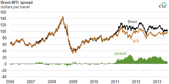
Please review Figure 1 and Figure 2 in Lesson 2 [89] to see the upward trend in oil production and the downward trend in oil imports for the same time period.
Crude oil transportation
The following links provide good resources for the U.S. pipeline infrastructure:
- U.S. Energy Mapping System [90]
- American Petroleum Institute (API) [91]
- The National Pipeline Mapping System [92]
Please go to this map on Pipeline 101.org [85] and find Cushing, OK.
More information about tankers can be found on this article, "Oil tanker sizes range from general purpose to ultra-large crude carriers on AFRA scale [86]", on the EIA website.
Figure 3 is drawn from the EIA data for the U.S. Crude Oil Refinery Receipts by mode of transportation in 2020. As you can see, pipelines transport the largest portion of domestic crude oil, and tankers transport the largest portion of foreign crude oil to the refineries.
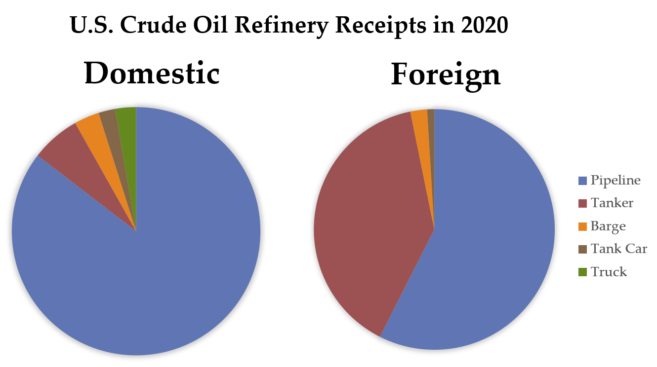
| Percent of Receipts | Domestic | Foreign |
|---|---|---|
| Pipeline | 85% | 56% |
| Tanker | 6% | 39% |
| Barge | 4% | 2% |
| Tank Car | 2% | 1% |
| Truck | 3% | 0% |
Crude Oil Refining
The following mini-lecture presents each phase of the crude oil refining process and the various products that are extracted from each barrel of oil.
Key Learning Points for the Mini-Lecture: Crude Oil Refining
While watching the mini-lecture, think about the following:
- products made from a barrel of crude oil
- refining process
- distillation
- conversion = “cracking,” reforming, alkylation, “coking”
- types of refined products
In the previous lesson, we talked about the actual logistics of getting crude oil to the refineries. And again, keep in mind, crude oil itself is not where the value lies, it's once the refiners turned it into various refined products and also petrochemical feedstocks.
Here's a picture of a petroleum refining complex down in Port Arthur, Texas, which is again, part of that huge refining petrochemical corridor along the US Gulf Coast. A map of where the current refineries are located, and this one is shaded in to show the petroleum administration defense districts, or the various PADDs, that we discussed in the prior lesson. Just a simple illustration of how the process might work. You can see these are seafloor gathering systems for crude oil, bringing through onshore, then you got offshore drilling and production platforms there. You can also see some tankers that are offloading and more than likely imported crude oil directly to the refineries.
The refining process itself, these are the types of products that you can extract from a simple barrel of crude oil. You can see gasoline being the largest, and then diesel being the second largest percentage. So, we have, again, basically, the largest component being motor fuels. Now the distillation process, it's the same as distilling anything. You're going to heat up the crude oil, and then naturally there's going to be some vapors, and some other moisture, or some other condensation, and they're all going to represent products that are derived from raw crude oil. So, you're going to separate heavier and lighter components by heating raw crude oil, feeding it into a distillation tower where the cooling occurs.
The lighter fractions rise to the top while heavier fractions remain on the bottom layers according to weight and boiling points. Again, we're talking about fractions, in other words, the hydrocarbon fractions that can be removed from the complex hydrocarbon molecule that is crude oil. The primary fractions come out of this first process of distillation but things like liquefied petroleum gases, or LPGs, naphtha, kerosene, diesel, heavy oils, and residual oil. And now, we have some other processes that all these will go through, processes like reforming, alkylation, cracking, and coking to make additional products that we might need.
And here's just illustration of the distillation column, and you can see off to the right the products that come out simply by heating up the crude oil in this first phase. One of the next phases, then, is conversion, and this is where they're going to crack the remaining heavy hydrocarbons into lighter once. You've got thermal cracking where heat or steam is actually used to break down larger hydrocarbons into smaller ones, or chemical cracking where a specific catalyst is used to speed up the cracking process. The result of the cracking process is to create additional gasoline, to create jet fuel and diesel fuel. Now, again, the overall process of a refinery is to take complex hydrocarbon molecules break them down, and then reform them into the products that the refinery chooses to market at any one time.
Again, the next phase in what we call the conversion process is the reformer. This is where you have heat, pressure, and catalysts that take these smaller molecules and combine them back into larger ones. For instance, naphtha, which is a product of the distillation phase, can be turned into gasoline. Another conversion process is that of alkylation. You take some of the lower weight molecules, and they're combined using a catalyst to form high-octane hydrocarbons for gasoline blending. This are the so-called anti-knocking compounds that are added to gasoline.
And then last, but not least, we have coking, which is another conversion process. Coking is where the residual oil, the heaviest stuff that comes from the distillation process, is going to be heated, and it's broken down into heavy oil, gasoline, and naphtha as well. The remaining product then is known as coke. It is used as a fuel source, it's used as iron ore smelting, and this is what is inside of dry cell batteries.
And then you have all-in-one the refining process. You can see here, you start off with the raw crude oil, you have the distillation column, the LPGs come off the top, you can see here, the naphtha can be sent to the reformer to create gasoline, then we have the cracking, the alkylation unit and last, but not least, the coking. So, all of these together combined form the refining process, which then gives us these various products that are going to be sold in places like retail, gasoline outlets, but then, also, there's going to be some of these that are used as feedstocks for the actual production of petrochemicals.
Optional Viewing
Petroleum Refining Basics video (10 minutes)
For crude oil to be used effectively by modern industry, it has to be separated into its component parts and have impurities like sulfur removed. The most common method of refining crude is the process of fractional distillation. This involves heating crude oil to about 350 degrees Celsius, to turn it into a mixture of gases. These are piped into a tall cylinder, known as a fractional tower.
Inside the tower, the very long carbon chain liquids, such as bitumen and paraffin wax, are piped away to be broken down elsewhere. The hydrocarbon gases rise up inside the tower, passing through a series of horizontal trays and baffles called bubble caps. The temperature at each tray is controlled so as to be at the exact temperature that a particular hydrocarbon will condense into a liquid. The distillation process is based on this fact.
Different hydrocarbons condense out of the gas cloud when the temperature drops below their specific boiling point. The higher the gas rises in the tower, the lower the temperature becomes. The precise details are different at every refinery and depend on the type of crude oil being distilled. But at around 260 degrees, diesel condenses out of the gas. At around 180 degrees, kerosene condenses out. Petrol, or gasoline, condenses out at around 110 degrees, while petroleum gas is drawn off at the top.
The distilled liquid from each level contains a mixture of alkanes, alkenes, and aromatic hydrocarbons with similar properties, and requires further refinement and processing to select specific molecules.
The quantities of the fractions initially produced in an oil refinery don't match up with what is needed by consumers. There is not much demand for the longer chain, high molecular weight hydrocarbons, but a large demand for those of lower molecular weight-- for example, petrol. A process called cracking is used to produce more of the lower molecular weight hydrocarbons. This process breaks up the longer chains into smaller ones.
There are many different industrial versions of cracking, but all rely on heating. When heated, the particles move much more quickly, and their rapid movement causes carbon-carbon bonds to break. The major forms of cracking are thermal cracking, catalytic, or cat cracking, steam cracking, and hydrocracking.
Because they differ in reaction conditions, the products of each type of cracking will vary. Most produce a mixture of saturated and unsaturated hydrocarbons. Thermal cracking is the simplest and oldest process. The mixture is heated to around 750 to 900 degrees Celsius, at a pressure of 700 kilopascals That is, around seven times atmospheric pressure. This process produces alkenes, such as ethene and propene, and leaves a heavy residue.
The most effective process in creating lighter alkanes is called catalytic cracking. The long carbon bonds are broken by being heated to around 500 degrees Celsius in an oxygen-free environment, in the presence of zeolite. This crystalline substance, made of aluminum, silicon, and oxygen, acts as a catalyst. A catalyst is a substance that speeds up a reaction or allows it to proceed at a lower temperature than would normally be required.
During the process, the catalyst, usually in the form of a powder, is treated and reused over and over again. Catalytic cracking is the major source of hydrocarbons, with 5 to 10 carbon atoms in the chain. The molecules most formed are the smaller alkanes used in petrol, such as propane, butane, pentane, hexane, heptane, and octane, the components of liquid petroleum gas.
In hydrocracking, crude oil is heated at very high pressure, usually around 5,000 kilopascals, in the presence of hydrogen, with a metallic catalyst such as platinum, nickel, or palladium. This process tends to produce saturated hydrocarbons, such as shorter carbon chain alkanes because it adds a hydrogen atom to alkanes and aromatic hydrocarbons. It is a major source of kerosene jet fuel, gasoline components, and LPG.
In one method, thermal steam cracking, the hydrocarbon is diluted with steam and then briefly heated in a very hot furnace, around 850 degrees Celsius, without oxygen. The reaction is only allowed to take place very briefly.
Light hydrocarbons break down to the lighter alkenes, including ethene, propene, and butene, which are useful for plastics manufacturing. Heavier hydrocarbons break down to some of these, but also give products rich in aromatic hydrocarbons and hydrocarbons suitable for inclusion in petrol or diesel. Higher cracking temperature favors the production of ethene and benzene.
In the coking unit, bitumen is heated and broken down into petrol alkanes and diesel fuel, leaving behind coke, a fused combination of carbon and ash. Coke can be used as a smokeless fuel.
Reforming involves the breaking of straight chain alkanes into branched alkanes. The branched chain alkanes in the 6 to 10 carbon atom range are preferred as car fuel. These alkanes vaporize easily in the engine's combustion chamber, without forming droplets and are less prone to premature ignition, which affects the engine's operation. Smaller hydrocarbons can also be treated to form longer carbon chain molecules in the refinery. This is done through the process of catalytic reforming, When heat is applied in the presence of a platinum catalyst, short carbon chain hydrocarbons can bind to form aromatics, used in making chemicals. A byproduct of the reaction is hydrogen gas, which can be used for hydrocracking.
Hydrocarbons have an important function in modern society, as fuel, as solvents, and as the building blocks of plastics. Crude oil is distilled into its basic components. The longer carbon chain hydrocarbons may be cracked to become more valuable, shorter chain hydrocarbons, and short chain molecules can bind to form useful longer chain molecules.
Cushing - NYMEX Crude Oil Hub
As explained in previous lessons, crude oil is one of the energy commodities that are traded on the NYMEX. Its symbol is CL. We refer to this as West Texas Intermediate or WTI crude. It is low sulfur, and so, therefore, is given the nickname sweet crude. The NYMEX contract for crude oil was initiated in 1983. Every contract represents 1,000 barrels, which is the equivalent of 42,000 gallons of oil. Price quotes on the New York Mercantile Exchange are all US dollars and cents per barrel. The minimum price fluctuation, the amount that the price has to move for a trade to take place, is one cent per barrel, or $10 per contract.
The delivery point for crude oil under this contract is what's known as FOB, or free on board, or delivered to the seller's facilities at Cushing, Oklahoma and to any pipeline or storage facility with access to Cushing Storage, TEPPCO, or Equilon pipelines. So, if you buy or sell crude oil contracts on NYMEX for a particular month, you are obligated to either receive the crude oil or deliver the crude oil at Cushing, Oklahoma.
The delivery point for the NYMEX Crude Oil contract is the Cushing Hub in Cushing, OK, USA. It is the world's largest crude oil storage facility and represents 16% of the US capacity. It has been in the news over the last few years as TransCanada seeks approval for its Keystone XL pipeline and, as the excess supply at Cushing looks for new outlets to the Gulf of Mexico refineries.
Key Learning Points for the Mini-Lecture: Cushing - NYMEX Crude Oil Hub
While watching the following mini-lecture, please keep in mind the following key points:
- Cushing, OK is the delivery "hub" for the NYMEX contract for crude oil.
- It has both pipelines and storage capacity.
- It is currently over-supplied.
- Takeaway capacity is constrained.
- Gulf Coast refiners are having to pay higher prices for imported crude as a result.
- Two major pipeline projects have helped move crude south.
- Keystone XL pipeline could bring more Canadian tar sands crude oil to Cushing.
NOTE:
The lecture slides can be found in the Modules under Lesson 3: The New York Mercantile Exchange (NYMEX) & Energy Contracts in Canvas.
In the last lesson, we talked about Cushing as the New York Mercantile Exchange crude oil hub for the buying and selling of physical crude products under the New York Mercantile Exchange contracts. We're going to talk a little bit about this. But I want to spend some time on it only because it's made the news a few times in the past year. There are certainly some issues related to pricing of crude oil, which again impacts the price of unleaded gasoline throughout the United States, involving Cushing and a surplus of crude oil that happens to be there.
Here are some aerial pictures of Cushing itself. It is a pipeline and above ground crude oil storage hub in Oklahoma. It is a pipeline hub. Hub-- we use the term whenever we're really talking about the intersection of multiple pipes where any type of crude, natural gas liquids, natural gas can be exchanged or moved from one pipe to another.
They also have, as the previous picture showed, it's a crude oil storage tank farm as well. It's the world's largest crude oil storage facility. The companies of TEPPCO, Equilon, and TransCanada have crude oil pipelines that run to and away from Cushing.
It has 46 million barrel storage capacity that represents 16% of the total US crude oil storage capacity. It's designed to receive Gulf Coast and Midwest crude, to store it, and then transport it to refineries in Oklahoma and throughout the upper Midwest. Some of the key companies that are participants and owners of facilities of Cushing are Enbridge, BP, SemGroup, ConocoPhillips, Sunoco, Plains All American, and TEPPCO.
Here, in the last couple years, there have been historically high inventory levels. In fact, they're running out of storage capacity for crude. There's no incremental storage capacity at present. In part, this is due to the dramatic increase in domestic production of crude oil from the shale plays.
The most recent ones are the Bakken Shale in North Dakota and the Mississippian Lime play in central or northern Oklahoma. The Canadian imports continue to increase. The Keystone XL pipeline received some press earlier this year. But a lot of people do not know that TransCanada already has a pipeline in place known as the Keystone pipeline. So, there are shipments of Canadian crude oil entering the United States, coming to Cushing as we speak.
One of the biggest issues, though, is that we can't get the surplus crude oil to the Gulf Coast. So, as a result, Gulf Coast refiners-- that's the largest petrochemical refining area in the United States-- are having to pay more for crude oil than the WTI price. They're having to import more.
And so, it's a price that is above WTI. It's not quite the North Sea Brent Crude pricing that occurs in Europe. But it's more than they should have to pay because we can't get this excess supply down to them.
A couple of solutions to this problem, this bottleneck or this glut of supply, is to reverse the Seaway pipeline. The Seaway pipeline has been in existence for several decades. It originally was a crude oil pipeline that brought crude that was offloaded from tankers near Houston in the Ship Channel and Beaumont-Port Arthur areas of eastern Texas, right there on the Gulf. And the pipeline shipped it up to Cushing from there. In the late '80s, early '90s, it was actually a natural gas pipeline, taking natural gas from the mid-continent down to the Houston Ship Channel petrochemical and refining corridor, and was later converted back to crude oil. And it currently would bring crude oil to Cushing.
However, the demand is actually in the Gulf of Mexico. So, Enbridge and Enterprise bought this pipeline from ConocoPhillips. It's 500 miles, runs from Freeport, Texas, up to Cushing, Oklahoma. And they have already reversed the flow, currently by, in essence, redirecting the pumps along the pipeline. They're able to push 150,000 barrels a day of crude oil from Cushing down towards the Gulf Coast refiners. They're working on a project to expand the pipeline. And hopefully, by next year, they'll be able to ship 400,000 barrels a day southbound to the Gulf Coast refineries.
The Keystone XL project is the one that has received some press in this past year. It's TransCanada Pipeline Company's proposed two-phase crude oil pipeline. The objective is to move tar sands, crude oil, from Canada's Alberta province all the way down to Texas.
Phase one would run from Alberta, Canada, to Cushing, Oklahoma, approximately 1,180 miles. Phase two would run from Cushing, Oklahoma, to Nederland, Texas, on the Gulf Coast. And that segment is about 435 miles.
This is a picture of the Seaway pipeline, as you can see running from Cushing all the way down to Freeport, Texas. And in fact, the flow on this has been reversed. And here's the Keystone XL project, the yellowish dotted lines, and, the existing Keystone pipeline, is in orange. And so, you can see that TransCanada plans phase one to hook up with a portion of the existing Keystone pipeline. But phase two would run from Cushing on down to both the Houston Ship Channel and Port Arthur, Texas.
Some of the project issue's, as I've already mentioned, Seaway pipeline. It's already reversed their pump stations. And it's flowing southward again already as we speak.
Keystone XL, phase one, requires a presidential permit for the international border crossing. Back in February, this was delayed by the US State Department because the pipeline route was going to go through a sensitive environmental area known as Sandhills in Nebraska. The TransCanada Keystone project's parent is investigating alternate routes, and in fact, I believe has refiled for the permit to get the international border crossing.
Phase two, the section from Cushing, Oklahoma, down to Texas, is going to proceed. TransCanada has already received most of the regulatory approvals that they need. As a crude oil pipeline, they can only receive common carrier status. They are not a utility. And so they will have to negotiate with landowners the entire way.
There is a new project that ONEOK, out of Tulsa, Oklahoma, has announced. They're going to build a crude oil pipeline, which will run from the Bakken Shale area in North Dakota all the way to Cushing. It's estimated to be somewhere between $1.5 to $1.8 billion and 1,300 miles of pipeline. And they hope to have it in service in approximately three years' time.
Summary and Final Tasks
Key Learning Points: Lesson 5
- There are various methods used to transport crude oil from the wellhead to the refinery.
- truck
- rail
- pipeline
- barge
- tanker
- Brent is the “global standard” crude oil stream, while WTI is the North American standard and is also the standard for futures trading in crude oil.
- PADDs are regional districts for supply and distribution of crude oil.
- The US still relies heavily on imported crude, but domestic supplies are increasing.
- The refining process consists of distillation and conversion and produces several products used in transportation and as petrochemical feedstocks.
Reminder - Complete all of the lesson tasks!
You have reached the end of this lesson, Double-check the list of requirements on the first page of this lesson to make sure you have completed all of the activities listed there before beginning the next lesson.
Lesson 6 - Natural Gas Logistics & Value Chain/US LNG Exports & Global Markets
Lesson 6 Introduction
Overview
Flow chart in the shape of an arrow.
Production & Gathering (Wellhead Cost, Gathering Fees, Fuel)
Leads to
Processing/Refining (processing fees, refining fees, inputs/outputs)
Leads to
Transmission (levels of service, tariffs, rates & fuel)
Leads to
Storage (levels of service, tariffs, rates of fuel)
Leads to
Distribution (utilities, end-users, residential, retail)
This graphic illustrates the various steps in the process of getting crude oil and natural gas from the wells all the way to market. As you can see, there is wellhead aggregation (production & gathering), the cleaning (processing and refining) of the raw stream, and production of valuable natural gas liquids (processing or refining), the transportation and storage, and finally, the distribution and retail delivery to the various end-users. As you will see, each step along this "path" will have some costs associated with it, and most will represent an opportunity for generating revenue. These will add to the total profit that can be derived from the initial wellhead product.
Watch the following video about natural gas (3:38 minutes).
PRESENTER: Natural gas-- natural gas is primarily methane or CH4 with smaller quantities of other hydrocarbons. It was formed millions of years ago when dead organisms sunk to the bottom of the ocean and were buried under deposits of sedimentary rock. Subject to intense heat and pressure, these organisms underwent a transformation in which they were converted to gas over millions of years.
Natural gas is found in underground rocks called reservoirs. The rocks have tiny spaces called pores that allow them to hold water, natural gas, and sometimes oil. The natural gas is trapped underground by impermeable rock called a cap rock and stays there until it is extracted.
Natural gas can be categorized as dry or wet. Dry gas is essentially gas that contains mostly methane. Wet gas, on the other hand, contains compounds such as ethane and butane in addition to methane. These natural gas liquids or NGLs for short can be separated and sold individually for various uses such as in refrigerants and to produce products like plastics.
Conventional natural gas can be extracted through drilling wells. Unconventional forms of natural gas like shale gas, tight gas, sour gas, and coal bed methane have specific extraction techniques. Natural gas can also be found in reservoirs with oil and is sometimes extracted alongside oil. This type of natural gas is called associated gas. In the past, associated gas was commonly flared or burned as a waste product, but in most places today it is captured and used.
Once extracted, natural gas is sent through small pipelines called gathering lines to processing plants, which separate the various hydrocarbons and fluids from the pure natural gas to produce what is known as pipeline quality dry natural gas before it can be transported. Processing involves four main steps to remove the various impurities-- oil and condensate removal, water removal, separation of natural gas liquids, sulfur, and carbon dioxide removal. Gas is then transported through pipelines called feeders to distribution centers or is stored in underground reservoirs for later use.
In some cases, gas is liquefied for shipping in large tankers across oceans. This type of gas is called liquefied natural gas or LNG. Natural gas is mostly used for domestic or industrial heating and to generate electricity. It could also be compressed and used to fuel vehicles and is a feedstock for fertilizers, hydrogen fuel cells, and other chemical processes.
Natural gas development, especially in the United States, has increased as a result of technological advances in horizontal drilling and hydraulic fracturing.
When natural gas is burned, there are fewer greenhouse gas emissions and air pollutants when compared to other fossil fuels. In fact, when used to produce electricity, natural gas emits approximately half the carbon emissions of coal. Despite fewer emissions, natural gas is still a source of CO2.
In addition, methane is a potent greenhouse gas itself, having nearly 24 times the impact of CO2. During the extraction and transportation process, natural gas can escape into the atmosphere and contribute to climate change. Natural gas leaks are also dangerous to nearby communities because it is a colorless, odorless, highly toxic, and highly explosive gas. That's natural gas.
Learning Outcomes
At the successful completion of this lesson, students should be able to:
- define the steps in the movement of natural gas from the wellhead to the end-user (“wellhead-to-burner tip” path);
- recognize the “value chain” along the path;
- explain the general methods of transporting natural gas from well to end-user:
- gathering,
- processing & Natural Gas Liquids (NGLs),
- pipeline,
- storage,
- distribution/end-use;
- describe both the domestic and global markets for LNG.
What is due for this lesson?
This lesson will take us one week to complete. The following items will be due Sunday, 11:59 p.m. Eastern Time.
- Lesson 6 Quiz
- Lesson 6 Activities as assigned in Canvas
Questions?
If you have any questions, please post them to our General Course Questions discussion forum (not email), located under Modules in Canvas. The TA and I will check that discussion forum daily to respond. While you are there, feel free to post your own responses if you, too, are able to help out a classmate.
Reading Assignment: Lesson 6
Reading Assignment:
From Wellhead to Burnertip
While reading each of these short descriptions, try to visualize the movement of the natural gas through each stage and what exactly is occurring. We will go into more detail for each of these steps in the mini-lectures.
Read the following sections on the NaturalGas.org [95] website.
- Natural Gas -- From Wellhead to Burner Tip tab:
- Exploration [96]
- Extraction [97]
- Production [98]
- Transport [99]
- Storage [100]
- Distribution [101]
- Marketing [102]
- Processing Natural Gas [103]
- A Brief History of Regulation [104]
Please go to this page "Understanding Henry Hub [105]" from the CME Group. Read the content on the page and watch the video (2:59).
Optional Reading and Viewing
Readings
Go to the EIA website and read the following sections from “Nonrenewable Sources [20]”:
- Natural Gas [7]
- Delivery and Storage [33]***
- Natural Gas Pipelines [106]***
- Where Our Natural Gas Comes From [34]
- Imports and Exports [35]
- How Much Gas Is Left [107]
- Use of Natural Gas [36]
- Natural Gas Prices [37]
- Natural Gas & the Environment [39]
- Liquefied Natural Gas (LNG) [108]****
Natural Gas 101 Video (3:38 minutes)
Natural gas-- natural gas is primarily methane or CH4 with smaller quantities of other hydrocarbons. It was formed millions of years ago when dead organisms sunk to the bottom of the ocean and were buried under deposits of sedimentary rock. Subject to intense heat and pressure, these organisms underwent a transformation in which they were converted to gas over millions of years.
Natural gas is found in underground rocks called reservoirs. The rocks have tiny spaces called pores that allow them to hold water, natural gas, and sometimes oil. The natural gas is trapped underground by impermeable rock called a cap rock and stays there until it is extracted.
Natural gas can be categorized as dry or wet. Dry gas is essentially gas that contains mostly methane. Wet gas, on the other hand, contains compounds such as ethane and butane in addition to methane. These natural gas liquids or NGLs for short can be separated and sold individually for various uses such as in refrigerants and to produce products like plastics.
Conventional natural gas can be extracted through drilling wells. Unconventional forms of natural gas like shale gas, tight gas, sour gas, and coalbed methane have specific extraction techniques. Natural gas can also be found in reservoirs with oil and is sometimes extracted alongside oil. This type of natural gas is called associated gas. In the past, associated gas was commonly flared or burned as a waste product, but in most places today it is captured and used.
Once extracted, natural gas is sent through small pipelines called gathering lines to processing plants, which separate the various hydrocarbons and fluids from the pure natural gas to produce what is known as pipeline quality dry natural gas before it can be transported. Processing involves four main steps to remove the various impurities-- oil and condensate removal, water removal, separation of natural gas liquids, sulfur and carbon dioxide removal. Gas is then transported through pipelines called feeders to distribution centers or is stored in underground reservoirs for later use.
In some cases, gas is liquefied for shipping in large tankers across oceans. This type of gas is called liquefied natural gas or LNG. Natural gas is mostly used for domestic or industrial heating and to generate electricity. It could also be compressed and used to fuel vehicles and is a feedstock for fertilizers, hydrogen fuel cells, and other chemical processes.
Natural gas development, especially in the United States, has increased as a result of technological advances in horizontal drilling and hydraulic fracturing.
When natural gas is burned, there are fewer greenhouse gas emissions and air pollutants when compared to other fossil fuels. In fact, when used to produce electricity, natural gas emits approximately half the carbon emissions of coal. Despite fewer emissions, natural gas is still a source of CO2.
In addition, methane is a potent greenhouse gas itself, having nearly 24 times the impact of CO2. During the extraction and transportation process, natural gas can escape into the atmosphere and contribute to climate change. Natural gas leaks are also dangerous to nearby communities because it is a colorless, odorless, highly toxic, and highly explosive gas. That's natural gas.
A History of Natural Gas Video (11:57 minutes)
Natural gas has enormous potential as a versatile energy source. While it's had a history of powering electric generators and heating stove-tops, it's growing in use as an efficient fuel that also powers cars and trucks. But what exactly is natural gas? Natural gas is a naturally occurring chemical, primarily made up of methane-- CH4. Its purity makes it an environmentally friendly fuel. Methane does not leave a residue when burned, so its emissions do not react with sunlight to create smog.
How Natural Gas is Formed
The natural gas we use today began as microscopic plants and animals living in the ocean tens of millions of years ago. As they thrived, they absorbed energy from the sun, which was stored as carbon molecules in their bodies. When they died, they sank to the bottom of the sea and were covered by layer after layer of sediment. As these plants and animals became buried deeper in the earth over millions of years, heat and pressure began to rise. The amount of pressure and degree of heat transformed the bio-matter into natural gas.
Where Natural Gas is Formed
After natural gas was formed it tended to migrate upward through tiny pores and cracks in the surrounding rock. Some natural gas seeped to the surface, while other deposits traveled upward until they were trapped under impermeable layers of rock such as shale or clay. These trapped deposits are where we find natural gas today. In 1859, Edwin Drake drilled the first commercial well in Titusville, Pennsylvania, striking natural gas and oil. This is considered by many to be the beginning of the natural gas industry.
First Uses of Natural Gas
For most of the 1800s, natural gas was used almost exclusively as a fuel for lamps. Because no pipeline network existed to transport large amounts of gas over long distances, most of the gas was used to light local city streets. It was moved through small bore lead pipe. Then in 1885, Robert Bunsen invented a burner that mixed air with natural gas. The Bunsen burner showed how gas could provide heat for cooking and warming buildings. After the 1890s, many cities began converting their street lamps to electricity forcing gas producers to look for new markets. But the lack of mobility to transport gas to consumers was still an issue.
Transporting Natural Gas
In the energy industry, natural gas was originally obtained as a byproduct from oil production. Since it was viewed as too costly to produce, much of it was burned off by flaring at the wellhead. Improvements in metals, welding techniques, and pipe-making during World War II, opened natural gas to new markets thanks to pipeline networks. Throughout the 1950s and 1960s, thousands of miles of pipeline were constructed throughout the United States.
Although natural gas was becoming economically attractive with a growing pipeline network, crude oil was still far more popular and more widely used as a source of energy. For years, the industry perception remained that supplies of natural gas were limited. Although natural gas had been discovered in tight rock formations called shale, it was deemed too expensive and difficult to harness.
Technology Advances
With advances in drilling technology, new solutions emerged that solved these issues. Horizontal drilling and hydraulic fracturing, commonly referred to as fracking, were introduced as innovative techniques to reach shale deposits and harvest natural gas. Originally pioneered in the 1940s and refined in the 1970s, these processes have revolutionized the industry.
After the well site has been carefully prepared to meet environmental health and safety standards, drilling can begin. This is an intricate operation requiring a well-planned infrastructure, a variety of processes, and expert well-trained specialists are used to bring natural gas to the surface. Chesapeake works with these experts during every aspect of the project, while strictly adhering to all individual state regulations.
During the drilling process, the rig is in constant operation 24 hours a day, seven days a week, for approximately 21 to 28 days. As an added precaution in some areas, a protective mat covers 2/3 of the pad site. Utilizing heavy duty industrial strength drill bits, a typical well is drilled in several stages, starting with a large diameter drill bit and then successively smaller drill bits as the drilling has advanced.
After drilling each portion of the well, nested steel protective casing is cemented into place. This will protect groundwater and maintain the integrity of the well. Initially, and prior to moving in the drilling rig, a large diameter hole is drilled for the first 50 to 80 feet. Conductor casing is then cemented into place, stabilizing the ground around the drilling rig and wellhead and isolating the well from most private water wells.
In the Marcellus area, the fresh water zone extends to approximately 800 feet below ground. The fresh water zone consists of porous sandstone and rock strata containing water within the pore space of the rock. Chesapeake utilizes air drilling until the hole is advanced to an average of 100 to 200 feet below the base of the fresh water zone. This provides added protection to the fresh water zone.
A series of compressors and boosters generate the air that is used to lift the rock cuttings in fresh water into steel bins. The rock cuttings are then disposed of within state guidelines and permits. The drilling equipment is retracted to the surface and stored for the second stage of drilling. To protect the integrity of the hole and to protect the surrounding deep fresh water zone, a second layer of steel casing called surface casing is installed and cemented inside the newly drilled hole and conductor casing.
Cement is pumped down through the surface casing and up along the sides of the well to provide a proper seal. This completely isolates the well from the deepest of private or municipal water wells. A blowout preventer is installed after the surface casing has been cemented. The blowout preventer is a series of high-pressure safety valves and seals attached to the top of the casing to control well pressure and prevent surface releases.
Next, a small drilling assembly is passed down through the surface casing. At the bottom of the casing, the bit drills through the float equipment and cement continuing its journey to the natural gas target area as deep as 8,000 feet below the surface. The drilling method employed below the surface casing uses drilling mud, which is a nonhazardous mixture based on bentonite clay or synthetic thickeners. In addition to lifting the rock cuttings out of the hole, drilling mud also helps to stabilize the hole, cool the drill bit, and control downhole pressure. A few hundred feet above the target shale, the drilling assembly comes to a stop.
The entire string is retracted to the surface to adjust the drilling assembly and install a special drilling tool. This tool allows Chesapeake to gradually turn the drill bit until a horizontal plane is reached. The remainder of the well is drilled in this horizontal plane while in contact with the gas producing shale. Drilling continues horizontally through the shale at lengths greater than 4,000 feet from the point where it entered the formation.
Once drilling is completed, the equipment is retracted to the surface. Then a smaller diameter casing called production casing is installed throughout the total length of the well. The production casing is cemented and secured in place by pumping cement down through the end of the casing. Depending on regional geologic conditions, the cement is pumped around the outside casing wall to approximately 2,500 feet above the producing shale formation or to the surface.
The cement creates a seal to ensure that formation fluids can only be produced via the production casing. After each layer of casing is installed, the well is pressure-tested to ensure its integrity for continued drilling. A cross-section of the well below the surface reveals several protective layers-- cement, conductor casing, cement, surface casing, drilling mud, production casing, and then production tubing through which the produced gas and water will flow. Seven layers of protection.
Horizontal drilling offers many advantages when compared to vertical drilling. Since horizontal wells contact more of the gas producing shale, fewer wells are needed to optimally develop a gas field. Multiple wells can be drilled from the same pad sites. For example, development of a 1,280 acre tract of land using conventional vertical drilling techniques could require as many as 32 vertical wells with each having its own pad site. However, one multi-well pad site with horizontal wells can effectively recover the same natural gas reserves from the 1,280 acre tract of land while reducing the overall surface disturbance by 90%.
Fracking is a technique that involves pumping water and sand at high pressure into shale formations. After drilling has been completed in a prospective location, the shale formation is perforated or punctured to prime it for the fracturing process. The area is then subjected to water and sand at high pressure to fracture the shale. Once fractured, sand is used to hold the small cracks and fissures open, releasing natural gas and allowing it to move up the wellbore to the surface. With this new technology, a land rush soon followed by gas producers to obtain the best locations in potential gas shale plays across the nation. More discoveries are made every year and new industry estimates now state that the US has a 100 year supply of natural gas.
Common Uses of Natural Gas Today
Today, natural gas is used all over the world as a versatile form of clean-burning energy. Common uses include heating homes and powering hot water heaters, dryers, and stovetops. But its ability to adapt to so many other needed areas have made it an ideal energy for making plastics, powering electric turbines, and commercial chillers that cool office buildings. When used as an automotive fuel, Compressed Natural Gas, or CNG, is a clean fuel that can power buses, trucks, and compact cars.
Natural gas has proven to be a clean, affordable, abundant alternative to gasoline and coal. 99% of the natural gas used in the US is produced at home in our own nation. With a variety of uses and new technology, natural gas is proving it's the energy of the future.
Natural Gas Pipelines Operations Video (8:45 minutes)
Because of its domestic abundance, low environmental emissions, and high energy content, natural gas has become a very popular and important fuel in North America. In these early years of the 21st century, about one quarter of America's daily energy need is met by natural gas, including heating, electric generation, and industrial feedstock used for making products such as plastics and fertilizer. As the population swells and with it the need for this cleaner burning fuel, so too must long-haul pipeline systems evolve and expand to keep pace with America's natural gas demand.
Recently, Americans used more than 22 trillion cubic feet of natural gas in a single year. That's a tremendous amount of energy when one considers that 1 trillion cubic feet of natural gas is enough to heat one million homes for 15 straight years. Long-haul pipelines are the critical link between the often lengthy distances separating natural gas supply and major market areas. These major transportation systems generally differ from local distribution pipelines in several ways, such as the material composition and diameter of the pipeline, larger diameter steel versus smaller diameter plastic, and higher operating pressures versus lower operating pressures.
When it comes to the operation of long-haul natural gas pipeline systems and the coexistence between the transportation systems and the public, operating companies place their focus in two primary areas-- providing reliable service to customers and further minimizing the relatively low risks associated with transporting a volatile fuel source under high pressure. Bureau of Transportation statistics records have historically and consistently shown that long-haul pipelines have the best transportation safety record in the United States.
| Transportation Type | Fatalities per 100,000 U.S. Residents |
|---|---|
| Air | .24 |
| Rail | .30 |
| Transit | .08 |
| Pipeline | .004 |
Pipeline system accidents, which are reported to PHMSA, are rare, particularly when one considers that trillions of cubic feet of natural gas transported each year. But the industry fully understands the potential impact of a damaged pipeline and takes many measures to both maintain pipeline systems and prevent these accidents from occurring. Clearly, even though long-haul pipes have the fewest accidents among all companies involved in transportation, there is no rest on the best in class laurels.
But one incident is one too many, and operators continually look for ways to improve the transportation of natural gas. The industry has built its solid safety record on a foundation of continuous improvement. And as a result, it has seen a percentage decrease in the number of significant incidents in the past 20 years while the amount of natural gas moved in that time frame increased dramatically.
Every step of the way, these long-haul pipeline systems are monitored around the clock by high-tech equipment and highly skilled employees. The basic process to transport natural gas long distances involves not only the specialized steel pipeline but related measurement and pressure regulating equipment, compressor stations that compress the natural gas molecules to facilitate the journey, and control centers that monitor major operating conditions around the clock. Companies also repeatedly communicate with those living near pipelines, emergency responders, and other important stakeholders through various methods while providing strategically located above-ground markers and other means to remind them of their mostly underground assets.
As natural gas travels through the pipeline system, it is pressurized to varying levels inside the long-haul pipes to facilitate its journey. This is accomplished by squeezing the natural gas molecules by pressure known as compression. Compression of the natural gas molecules serves a twofold purpose. One, it reduces the size of the natural gas molecule by many times, thus increasing the amount of natural gas that can be transported in a given sized pipe. And two, it provides a propellant force or boost to help move the natural gas through the pipeline system.
Typically, compression of the natural gas molecules is required periodically along the route. This is accomplished by compressor stations usually placed at 40 to 100 mile intervals along the route. The natural gas enters the compressor station, or booster station as it's also called, where it is recompressed mechanically and propelled toward the next active compressor station where the process repeats. As a result, the highly pressurized natural gas moves through the pipelines at an average of about 10 to 20 miles per hour.
Along its journey, measurement and/or regulating stations are placed periodically to help manage the flow of natural gas entering or leaving the pipeline. At these stations, mechanical pressure regulators are used as necessary to reduce the pressure inside the pipeline to match customer needs. This facilitates the transfer of natural gas to industrial customers and the distribution companies that deliver the product to millions of homes and businesses each day.
The transportation of natural gas is often closely linked with the temporary storage of the commodity in porous rock formations or salt caverns deep underground. The underground geologic formations and associated above-ground operations equipment are connected by pipeline to various mainline systems. Natural gas storage facilities are important because they can temporarily hold large volumes of natural gas for later withdrawal during periods of high customer demand.
In order to manage the natural gas that enters the pipeline and to ensure shippers receive the transportation and/or storage services that they've contracted for, sophisticated control systems are required. Centralized natural gas control operations manned by trained operators continuously collect, assimilate, and manage data received from measurement, monitoring, and compression facilities all along the pipe. Most of the data received by a natural gas control center is provided by supervisory control and data acquisition systems, better known as SCADA.
SCADA is a sophisticated communication system that operates in real time with very little lag between measurements taken and the relay of the data to the natural gas control center. Measurements monitored and relayed include natural gas flow rates, operational pressures, and temperature readings, all of which are important to the assessment of the status of the pipeline at any given time. Alarms at these remote locations are also relayed to the control system operators. It's important for operators in the center to know what is happening along the pipeline system at all times. This allows for quick reaction to address and adjust to changing operating conditions.
Operators with these computer monitoring SCADA systems often have the ability to remotely operate certain equipment along the route, such as compressor station engines or valves. But these operator actions are limited by safeguards and redundant devices. Adjusting compressor engines allows for the quick and easy adjustment of flow rates in the pipeline, while remote operation of valves allow for the isolation of certain sections of pipeline for maintenance or emergency response purposes in coordination with local operating personnel.
Remote operating capability plus the strategic local area or regional placement of trained employees makes for the effective management and control of these long-haul natural gas transportation systems. For more information about long-haul natural gas pipelines, please visit the Interstate Natural Gas Association of America website at www.ingaa.org [110].
Natural Gas Liquids Video (11:14 minutes)
Hello, I’m Dan Brockett. I'm a member of the Shale Energy Education Team. And I work for Penn State Cooperative Extension. Today, I'm going to be talking a little bit about natural gas liquids.
[Slide]: Natural gas Liquids (NGL’s) are found in “wet gas” areas of shale gas producing regions.
[Dan]: I'm going to try to answer a few questions about natural gas liquids, like what is it, where is it, and why does it have added value. Then we're going to take a look at how NGLs are produced and processed, from wellhead to fractionation. Finally, we'll talk a little bit about how NGLs are used, and a bit of news regarding the future of NGLs in the Appalachian basin.
This map shows a portion of the Appalachian basin that contains Marcellus Utica and upper Devonian shale gas. You'll see the red line further east shows approximate Marcellus and upper Devonian wet-dry dividing line. The middle line shows approximate Utica Point Pleasant wet-dry line. And the line furthest west shows oil. For today's purposes, we're only talking about wet gas. And remember that these are only estimates of where these products are located.
[Slide]: Natural Gas Liquids: Each successive NGL has an additional carbon molecule and different chemical properties.
C1H4 – Methane (dry gas)
C2H6- Ethane
C3H8 – Propane
C4H10 – Butane (and Isobutane)
C5H12 – Pentane (natural gasoline)
[Dan]: Each successive natural gas liquid has additional carbon molecule and different chemical properties. Starting from the top, C1H4 is methane. That's referred to as dry gas, and generically referred to as natural gas. This is what we might expect to be piped into our homes and used to generate electricity.
All of those remaining hydrocarbons-- ethane, propane, butane, and iso-butane, and pentane-- are referred to as natural gas liquids. Natural gas liquids have added value based on BTU.
[Slide]:
| Gas | Net BTU Value | Typical Volume (more to less) |
|---|---|---|
| Methane | 1,011 | more |
| Ethane | 1,783 | |
| Propane | 2,572 | |
| Butane | 3,225 | |
| Pentane | 3,981 | |
| Hexane | 4,667 | less |
BTU stands for British thermal unit. To give you some scale, 1 BTU equals approximately lighting one match and letting it burn to the bottom. So you can see that methane, our dry gas, has about 1,000 BTUs, where ethane is about 1,800 BTUs.
As those hydrocarbons get heavier, they contain more BTUs. You will also note the typical volume that comes out of a well in the Appalachian basin in the wet gas region contains more methane than ethane, more ethane than propane, et cetera. So lighter gases tend to be produced more often than heavier gases.
Pipeline specification regarding those BTUs. Interstate pipelines require less than approximately 1,100 BTUs per SCF. SCF may not be a common term for you. It stands for standard cubic feet. Standard conditions are normally set around 60 degrees Fahrenheit and about 14.7 pressure at sea level.
Now, unprocessed wet gas is often well over 1,200 BTUs. And even when those heavier hydrocarbons, like propane, butane, and pentane, are removed, the BTU content still often exceeds 1,100. Some ethane then needs to be removed to meet pipeline specifications while the rest of the ethane may be rejected if there's not a market. Rejected ethane does not mean that it's thrown away. It's simply added to the gas stream, and contributes higher BTUs.
To give you an example of price, if there are processing facilities in a pipeline to market, then the price received tends to be significantly higher because those products can be separated and sold at their best and highest use. The other way natural gas liquids are often sold are in batches. They're sold as batches and separated from dry methane gas, but not separated into their each individual components.
[Slide]
Liquids Price Impact Example, assuming 1250 btu gas)
Category 1: Natural Gas = $2.00. Rich Gas increment = additional $.50 for a total of $2.50/MCF
Category 2: Natural Gas assumes 30-% shrinkage to $1.40. The Rich gas increments are divided into ethane, propane, iso-butane, butane and natural gasoline for a total of $3.21 /MCF
[Dan]: So now, let's talk about the process of how these natural gas liquids fall out of the gas stream. Pressure and temperature causes the heaviest hydrocarbons to fall out of the gas stream as liquids at the wellhead.
What is condensate? In this case, we'll refer to it as field condensate because it comes from the field where the gas is being produced. These condensates are a group of hydrocarbons that don't fit easily in the mainstream product categories. Usually, we're talking about pentane (C5)plus. The lower the number is, the heavier the condensate is. And generally, the heavier, the better the price.
Now, everything in this scale is compared to water, which is a 10. A number higher than 10 floats on top of water. Lower than 10, sinks. This graphic demonstrates that. As you can see on the left, lighter to heavier. And on the right, those products-- propane is lighter than butane, which is lighter than pentane, et cetera.
[Slide]:Density of Liquids
The API gravity goes from lighter to heavier in the following list:
Propane, Butane and Isobutane, Pentane, Hexane, Heptane
[Dan]: The next step in the process is a compressor station. The purpose of a compressor station is to add pressure to get gas to an interstate pipeline or to go to further processing. As you might guess, a compressor station adds pressure, which causes more liquids to fall out. We'll refer to these liquids as natural gasoline or drip gas. In this picture, you can see that center tower is water that's fallen out of the system, whereas the four towers outside of the center contain that natural gasoline.
The next step in the process is the cryogenic expansion process. If it's economic to extract ethane, cryogenic processes are required for high recovery rate. Essentially, cryogenic processes consist of dropping the temperature of the gas stream to about minus 120 degrees Fahrenheit.
Now, this is going to condense most of the natural gas liquids while methane will stay a gas. This separates most of the wet gas from the dry gas, but does not separate all the components of natural gas liquids. In order to do that, it requires fractionation.
Now, you can see in this graphic, our mixed natural gas liquids come in on a pipeline. And then they go through a series of towers that have different pressure and temperatures. The boiling point will only be reached by one product per tower. So you have a de-ethanizer, a de-propanizer, a de-butanizer, a de-isobutanizer.
And what comes out at the end is condensate. We'll refer to this as plant condensate. Generally, pentane plus. This is a picture of a fractionation plant in Houston, Pennsylvania. That's in Washington County.
Now, let's talk about how natural gas liquids are used. The most plentiful of the natural gas liquids is ethane. And it's predominantly used as a petrochemical feedstock. We're going to talk more about that later. There is a portion of ethane that's used as a heating fuel source. That's only when it's mixed with methane or propane.
Next, we'll talk about propane. About 35% of propane is used as a petrochemical feedstock. The majority of propane is used as a heating fuel source. You might be familiar with that as a heating source in your home, or barbecue, or for drying corn or lumber-- things like that. Also, about 10% of propane is exported. Butane-- about 22% of that is used as a petrochemical feedstock.
About 10% is exported, but the bulk of butane is used as a blend stock for motor gasoline. Iso-butane is entirely used as a blend stock for motor gasoline. Or natural gasoline-- that's pentane plus-- about 10% is used as a petrochemical feedstock. About 10% is exported. The majority of it goes as a blend stock for motor gasoline, and 8% to 10% is used for ethanol denaturing.
The infrastructure for ethane markets is very important, because it's the most plentiful of the natural gas liquids. Just a few years ago, there wasn't an outlet for ethane in the Appalachian basin. But quickly, pipelines were built to the Gulf Coast, where there are many cracker plants, also to Sarnia, Ontario, where there are a few cracker plants, and most recently to the Marcus Hook facility.
There's a pipeline that goes across southern Pennsylvania, taking that to an export facility, where it's placed on a ship and exported overseas. There's also a local option that may develop in the next four to five years in terms of developing cracker plants in the Appalachian basin.
So the ethylene chain goes from natural gas. Those products are then separated, fractionated. And you might have purity ethane that comes out. That purity ethane goes to a cracker plant. At that cracker plant, that purity ethane is turned into ethylene. Ethylene is further refined into intermediate products like PVC, vinyl chloride, styrene, and polystyrene. And those products are used to make adhesive, tires, footwear, bottles, caps-- a lot of things that are used as everyday products.
The future of natural gas liquids in the Appalachian basin. Well, there are some outlets for ethane and other natural gas liquids now, but those opportunities are growing. And more outlets for ethane, including additional pipelines to Sarnia, additional exports, and additional pipelines to the Gulf Coast. But this also includes an announcement from Shell to build an ethane-only cracker plant in Beaver County, Pennsylvania.
I'd like to give some credit to those folks who contributed to this presentation, including the Penn State Marcellus Center for outreach and research, Jim Ladlee at Penn State, Wikipedia, engineeringtoolbox.com, photos from MPLX and from the American Chemistry Counsel, and a map from EIA. If you would like more information on natural gas liquids or anything else regarding natural gas, please go to our website-- naturalgas.psu.edu. And thank you, very much.
How a Gas Turbine Works Video (2:39 minutes)
PRESENTER: Air-- a lot of gaseous molecules floating all around us. It's great for breathing, and it turns out it's great for getting lights turned on. That's because air along with abundant natural gas or other fuels are the ingredients that combine in a gas turbine to spin the generator that produces electric current. If you follow the electricity you use at home or at work, back through the power lines to your local power plant, you'll see that the process most likely starts with the work of the gas turbine, the very heart of the power plant.
First, air is drawn in through one end of the turbine. In the compressor section of the turbine, all those air molecules are squeezed together, similar to a bicycle pump squeezing air into a tire. As the air is squeezed, it gets hotter, and the pressure increases.
Next, fuel is injected into the combustor, where it mixes with a hot compressed air and is burned. This is chemical energy at work. Essentially, this is what happens in your family car's engine, but at about 2,900 times more horsepower.
Actually, it's exactly like the turbine engines on jet airplanes. The hot gas created from the ignited mixture, moves through the turbine blades, forcing them to spin at more than 3,000 RPMs. Chemical energy has now been converted into mechanical energy. The turbine then captures energy from the expanding gas, which causes the drive shaft, which is connected to the generator, to rotate.
That generator has a large magnet surrounded by coils of copper wire. When that magnet gets rotating fast, it creates a powerful magnetic field that lines up electrons around the coils and causes them to move. The rotating mechanical energy has now been converted into electrical energy because the movement of electrons through a wire is electricity. In what's called a combined cycle power plant, the gas turbine can be used in combination with a steam turbine to generate 50% more power. The hot exhaust generated from the gas turbine is used to create steam at a boiler, which then spins the steam turbine blades with their own drive shaft that turns the generator. What you end up with is the most efficient system for converting fuel into energy. And that's your GE Gas Turbine 101.
How does a Steam Turbine Work? Video (5:42 minutes)
Nuclear and coal-based thermal power plants together produce almost half of the world's power. Steam turbines lie at the heart of these power plants. They convert thermal energy in the steam to mechanical energy. This video will explain the inner workings of the steam turbines and why they are constructed in the manner they are in a step-by-step, logical manner.
To understand its basic workings, let's first observe one of their blades. You can see that the blade of a steam turbine has an airfoil shape. When the high-energy fluid passes over it, this airfoil shape will create a pressure difference.
This will subsequently create lift force. The lift force will rotate the turbine. In short, the energy in the fluid transfers to the mechanical energy of the rotor. (Flow energy > Mechanical energy)
To further understand steam turbine operation, let's understand fluid energy in greater depth. A fluid has three forms of energy due to its speed (kinetic energy), pressure, and temperature. As the blades absorb energy from the fluid, all three forms of energy come down.
The low-velocity jet is of no use to produce effective lift force. To increase velocity, the fluid is passed through a stator section. The stator set is stationary and attached to the turbine casing. You can see that flow area decreases along the stator, and the speed thus increases.
In short, the stator acts like a nozzle. As the speed of the jet increases in the stator, kinetic energy increases. As there is no net energy transfer in the fluid and stator section, the pressure and temperature of the jet should decrease to keep the total energy constant.
Now the next row of rotors is added. The stator also makes sure that the flow coming out of it will be at an optimum angle of attack to the next rotor set. After that, another nozzle set is added. Many such sets are used in a steam turbine.
There is an important term while designing steam turbines-- namely, degree of reaction. This term is calculated by dividing pressure and temperature energy by the total energy change in the rotor. Pressure and temperature energy together is called enthalpy. The degree of reaction decides what type of steam turbine it is.
As the pressure of the steam undergoes a drastic reduction during steam turbine operation, its volume increases proportionally. To accommodate such an expanded steam we have to increase the flow area. Otherwise, the flow speed will become too high. This is the reason why the steam turbine blades are too long towards the outlet.
You can see how long the last stage turbine blades are compared to the first stage blades. The tips of such long blades will have very high velocity compared to the root. A twist has given to it so that all blade cross-sections will remain at an optimum angle of attack.
This kind of large turbine uses two such symmetrical units. You can see how the steam is equally divided between these units. High-capacity power plants use different stages of steam turbines, such as high-pressure turbines, intermediate-pressure turbines, and low-pressure turbines.
All these units are attached to a single rotating shaft. The shaft in turn, is connected to a generator. The reason for such different stages is quite interesting. With greater steam temperature comes greater power plant efficiency. This is according to the second law of thermodynamics.
But we cannot have temperature greater than 600 degrees Celsius since the turbine blade material will not withstand temperature more than that. The temperature of the steam decreases as it flows along the rows of the blade. Consequently, a great way to increase power plant efficiency is to add more heat after the first stage.
So after the first stage, the steam is bypassed to the boiler, and more heat is added. This is known as reheating. This will increase the steam temperature again, leading to higher plant efficiency and output.
One challenging problem in power plant operation is to keep the speed of the steam turbine constant. This is important since frequency of the electricity produced is directly proportional to the generator speed. However, depending on the load or power demand, the steam turbine speed will vary. To keep the steam turbine speed constant, a steam flow governing mechanism is used.
If a steam turbine rotates at a higher speed, the control valve will automatically reduce the steam flow rate to the turbine until the speed becomes normal. If a turbine rotates at a low speed, the inverse will be done. In this way, the balance of power demand and power supply will be perfectly synchronized.
To learn more about degree of reaction and its implications, please check the next video. Please help us at Patreon.com so that we can add one more member to the team, and we will be able to release two educational videos per month. Thank you.
Liquefied Natural Gas (LNG) 101 Video (2:23 minutes)
LNG, Liquefied Natural Gas. LNG is natural gas that has been cooled to at least minus 162 degrees Celsius to transform the gas into a liquid for transportation purposes.
To understand why liquefying natural gas is important, we first need to understand natural gas's physical properties. Methane has a very low density and is therefore costly to transport and store. When natural gas is liquefied, it occupies 600 times less space than as a gas.
Normal gas pipelines can be used to transport gas on land or for short ocean crossings. However, long distances and overseas transport of natural gas via pipeline is not economically feasible. Liquefying natural gas makes it possible to transport gas where pipelines cannot be built, for example, across the ocean.
The four main elements of the LNG value chain are, one, exploration and production, two, liquefaction, three, shipping, four, storage and regasification. At the receiving terminal, LNG is unloaded and stored before being regasified and transported by pipe to the end users.
The demand for LNG is rising in markets with limited domestic gas production or pipeline imports. This increase is primarily from growing Asian economies, particularly driven by their desire for cleaner fuels and by the shutdown of nuclear power plants.
The largest producer of LNG in the world is Qatar with a liquefaction capacity in 2013 of roughly one-quarter of the global LNG production. Japan has always been the largest importer of LNG and in 2013 consumed over 37% of global LNG trade.
The extraction process also has environmental and social issues to consider. LNG projects require large energy imports for liquefaction and regasification and therefore have associated greenhouse gas emissions.
Spills pose concerns to local communities. There have been two accidents connected to LNG. But in general, liquefaction, LNG shipping, storage, and regasification have proven to be safe. LNG projects require large upfront capital investments, which can be a challenge in moving projects ahead.
That's LNG.
Gathering and Compression
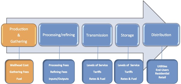
The first step in the movement of natural gas from the “wellhead-to-burner tip” is to determine the "deliverability," or sales volume of the well and then get it connected to a pipeline. This is normally done by midstream companies who gather wells together and deliver the gas to processing plants or directly into transmission pipelines.
The following mini-lecture explains these concepts in detail.
Key Learning Points for the Mini-Lecture: Gathering and Compression
While watching the mini-lecture, keep in mind the following questions:
- Why is the "deliverability" of a well important?
- What functions are performed by the Gatherer?
- Who are Producers and Operators?
- What are Compressors and how/why are they used?
Mini-lecture: Gathering & Compression (9:25 minutes)
In this lesson, we're going to talk about the entire logistics and value chain, now, for natural gas since we've already covered the one for crude oil itself. And the phrase we tend to use for this is wellhead to burner tip.
On the left is just a picture of a low-pressure well, kind of a small well. That's known as a Christmas tree-- the configuration of the various valves. And to the right is what's known as an oil/gas separator. First thing that happens when the raw natural gas comes out of the ground is to separate the heavier components, the oily substances, which, in essence, are what we call condensate.
Here's a schematic just kind of showing the overall industry and the different paths that the natural gas goes through. You can see you've got the gas well. You're going to have separation between oil, water, and natural gas. It's going to go through gas processing plants. There are some opportunities for storage here. And then, ultimately, it's going to get to the end users.
Here's sort of another setup of kind of how we separate upstream, midstream, and downstream within the natural gas industry. The upstream is, obviously, the production portion of it. Gathering, processing, and transmission and even storage are considered midstream along with the trading-type functions. And then, ultimately, downstream is going to be the actual end users for that.
Some of the players, some of the labels that we talk about on the various participants-- you've got operators and producers at the wellheads. You have the processing plant, which is your midstream companies-- they're gatherers and processors-- storage operators, which, a lot of times, can be independent storage. Or they can be pipeline and storage operators.
And then we have what's known as the city gate, which, really, is the distribution point, where the gas company, or LDC, picks up the gas from the transmission system and distributes to all of its customers.
So we're going to start at the wellhead. This is the production. This is what we're interested in once the well is completed, starts producing. We're interested in how much volume can be sold on a daily basis. This is known as the deliverability.
Now, this depends on the type of reservoir that you have. Some reservoirs, once they start producing, cannot be shut in. That is, they can't be turned off because you can actually lose the production.
Also the operator of the well. There's an entity or participant who actually operates the well. That means they are responsible for the day-to-day operations of the well. They also have an interest in the well. When we talk about working interest donors, those are the ones who actually have invested in the well and have an ongoing investment commitment to any operational costs. Now, the operator is also a working interest donor.
And then the joint operating agreement, or JOA, is the contract between the operator of the well and the various working interest owners. And it spells out exactly how things are going to happen, shared costs, how revenue is going to be dispersed, and those types of things.
Again, because we're interested in the production of the deliverability-- these are the sales volumes, again, so we want to know what are the ways in which we could actually increase the amount of gas flowing from a natural gas well. Well, I think by now, we're all familiar with horizontal drilling. Horizontal drilling allows you to pull more out of the reservoir than straight vertical drilling.
Another method would be to, basically, drill another well, or what we call in-field drilling-- go ahead and drill an offset well.
Wells that start to decline-- there can be a recompletion. Now, that can be two different things. Recompletion can be where you go down in, and you attempt to do something additional to the existing reservoir. Or you find another reservoir-- another layer, another producing zone-- and you go back down, and you complete that.
Of course, fracking is a form of initial releasing of the production. It can also be done multiple times if you think that there's more to be released.
Acid is one of the ways in which wells are completed. It's an older method instead of fracturing. But if you have a well that's in decline, then you may agree as a producer and an operator together to go ahead and try and use some acid to free it up. This works mainly in places like sand formations.
Compression. Now, compression is going to be another thing where you can use natural gas compressors to draw additional gas up out of the reservoir once the reservoir pressure itself has dropped to the point where the gas can't just free flow into the connected pipeline.
And the other course is to look for what we would call a low pressure connect. This is generally a service that's provided by midstream gatherers and processors, where they have compression at their plant, which can draw the gas from your well if the pressure of your well can't by itself exceed the pressure of the pipeline that it's connected to.
The quality of the gas-- this is very important because it's going to end up in a pipeline, and then, eventually, some type of end user whether it's a power plant, or it's someone's home hot water heater. And so a couple of things here initially.
The Btu value-- this is what we're after. This is what we sell. It's the heating content, a British thermal unit. That's the amount of energy required to raise 1 pound of water one degree Fahrenheit. Again, this is what we are marketing.
Water vapor. We don't want water in the gas stream nor to the pipelines.
Any types of corrosives-- there is sulfur, which naturally occurs in the raw natural gas down in a well. It can actually lead to the formation of hydrogen sulfide, which is a corrosive. That is, it can eat away at the steel pipe.
Nitrogen itself just takes up space. It has, obviously, no heating content. The same thing with CO2. Carbon dioxide just takes up space in the pipe. And so you don't want these inerts in there because you want to fill that pipeline up with as much heating content as you can.
And then the question of whether or not the gas is processable. In other words, can it be processed. Is the Btu content high enough to extract natural gas liquids, which are valuable on their own.
The other side of that question, really, is does it need processing. The pipelines are only going to accept a certain maximum amount of Btu content. If you think about it, something volatile, like propane, which I think we're all fairly familiar with-- you can't have that in someone's home hot water heater. You also can't inject propane into a boiler at a power plant. You will literally have an explosion.
And then any other kind of treatments.
Just some of the folks that I've already mentioned-- these are your wellhead participants. A producer has a working interest in the well. They're known as working interest donors. That means-- let's say, for instance, a particular well-- you had 10 owners. Everyone essentially contributed 10% of capital up front to drill the well. And now, because they're working interest owners, they are on the hook for any additional operating costs or investment of things like the recompletion of a well or drilling an offset well.
So, as a result of that, they're entitled to 10% of the production coming out of the reserves of the natural gas well. And so we refer to that as their entitlement.
As I mentioned before, the operator is also a working interest donor. They've got a percent of reserves, or their entitlement. They are responsible for the day-to-day operations.
They're also responsible for what we call well balancing or allocations. In other words, if you've got 10 owners-- if that well plays out eventually-- in other words, it's depleted-- then every one of those owners should have at some point in time received their 10% of those reserves that are in the ground.
If not, then the operator has to cash balance that out so that everyone is on a equal basis at the end. Otherwise, this is-- we have a considerable number of lawsuits over these types of things.
And as I mentioned previously, the operator initiates this joint operating agreement among all the working interest owners.
Here's just a quick diagram of how these things might be set up in the field. You've got gathering lines. They're going to come to a central point, a common point, and then go into a pipeline. Generally speaking, this pipeline is going to go to a processing plant so that the gas can be cleaned up as well as natural gas liquids extracted.
In terms of how you would connect these, a question might be whether or not you do need compression. And that's going to be a function of the pressure downstream into the pipe in which you wish to flow your gas.
And then we have to also recognize that there's going to be costs. The more compression that you use that you have to boost up the pressure of your well relative to the downstream pipeline-- it's done in stages, and there's going to be a cost. A lot of them run on natural gas. Some run electricity. So there is a cost inherent there, not to mention just the regular O&M-type costs.
Connect costs. You're going to have to eventually connect your well, and there's usually a fee of some kind. These are referred to as taps.
And then most pipeline companies these days require what's known as electronic flow measurement. They want to be able to see from a remote location how much gas is actually flowing in. And then, again, in terms of the point at which you connect to a downstream pipeline, there may be additional treatment that may be needed at that spot. And either you pay for that up front, or the pipeline or a midstream company may do that.
Here's just a quick picture here of some compressors. This is what's known as a horizontal compressor. The actual pistons that draw the gas in and push you back out are, in fact, laid out horizontally.
Compressors themselves-- they are two parts. You've got these large-diameter pistons, and those are the ones that draw the gas in and push it out-- in other words, increase the pressure by using these pistons. And these are driven by a crankshaft.
The other part is, really, an internal combustion engine. A lot of these resemble large diesel engines you might find in a semi tractor-trailer. And as I mentioned before, if you're using natural gas there in the field, then there is a cost of that, the cost of that gas. Because you're not able to market it, you are actually consuming it at your pad site. Or if you're running electric compression, there's going to be a charge by the electric utility.
The best way to think about these is if you've ever seen one of those little electric Black & Decker machines you might have in your garage that inflates car tires, bicycle tires, et cetera. There is literally a little piston in there that's moving in and out at about 1,000 times a second, and it is taking the air at roughly atmospheric pressure-- 14.75 pounds per square inch-- and boosting it up to-- let's say, for instance, in terms of car tires-- it may be anywhere from 32 to 40 pounds per square inch.
And then just here are some more compressors. The upper left and the lower left-- these would be at a well site, at a small well, whereas the upper right would be at a central location, sort of that common point that I showed you in a diagram a few slides back. It would be drawing in gas from multiple wells out in the field.
Now, the lower right-- that's actually a turbine compressor. A turbine compressor is literally a jet engine-type of setup with fan blades and everything else running at a very high speed using natural gas. Now, a turbine compressor generally is going to be used at a processing plant to circulate the gas through it. This would be a very, very large-scale version of little turbines that might be added to car engines or turbo diesel-type of engines.
Optional Viewing
A History of Natural Gas by Chesapeake Energy (11:58 minutes)
Natural gas has enormous potential as a versatile energy source. While it's had a history of powering electric generators and heating stove-tops, it's growing in use as an efficient fuel that also powers cars and trucks. But what exactly is natural gas? Natural gas is a naturally occurring chemical, primarily made up of methane-- CH4. Its purity makes it an environmentally friendly fuel. Methane does not leave a residue when burned, so its emissions do not react with sunlight to create smog.
How Natural Gas is Formed
The natural gas we use today began as microscopic plants and animals living in the ocean tens of millions of years ago. As they thrived, they absorbed energy from the sun, which was stored as carbon molecules in their bodies. When they died, they sank to the bottom of the sea and were covered by layer after layer of sediment. As these plants and animals became buried deeper in the earth over millions of years, heat and pressure began to rise. The amount of pressure and degree of heat transformed the bio-matter into natural gas.
Where Natural Gas is Formed
After natural gas was formed it tended to migrate upward through tiny pores and cracks in the surrounding rock. Some natural gas seeped to the surface, while other deposits traveled upward until they were trapped under impermeable layers of rock such as shale or clay. These trapped deposits are where we find natural gas today. In 1859, Edwin Drake drilled the first commercial well in Titusville, Pennsylvania, striking natural gas and oil. This is considered by many to be the beginning of the natural gas industry.
First Uses of Natural Gas
For most of the 1800s, natural gas was used almost exclusively as a fuel for lamps. Because no pipeline network existed to transport large amounts of gas over long distances, most of the gas was used to light local city streets. It was moved through small bore lead pipe. Then in 1885, Robert Bunsen invented a burner that mixed air with natural gas. The Bunsen burner showed how gas could provide heat for cooking and warming buildings. After the 1890s, many cities began converting their street lamps to electricity forcing gas producers to look for new markets. But the lack of mobility to transport gas to consumers was still an issue.
Transporting Natural Gas
In the energy industry, natural gas was originally obtained as a byproduct of oil production. Since it was viewed as too costly to produce, much of it was burned off by flaring at the wellhead. Improvements in metals, welding techniques, and pipe-making during World War II, opened natural gas to new markets thanks to pipeline networks. Throughout the 1950s and 1960s, thousands of miles of pipeline were constructed throughout the United States.
Although natural gas was becoming economically attractive with a growing pipeline network, crude oil was still far more popular and more widely used as a source of energy. For years, the industry perception remained that supplies of natural gas were limited. Although natural gas had been discovered in tight rock formations called shale, it was deemed too expensive and difficult to harness.
Technology Advances
With advances in drilling technology, new solutions emerged that solved these issues. Horizontal drilling and hydraulic fracturing, commonly referred to as fracking, were introduced as innovative techniques to reach shale deposits and harvest natural gas. Originally pioneered in the 1940s and refined in the 1970s, these processes have revolutionized the industry.
After the well site has been carefully prepared to meet environmental health and safety standards drilling can begin. This is an intricate operation requiring a well-planned infrastructure, a variety of processes, and expert well-trained specialists are used to bring natural gas to the surface. Chesapeake works with these experts during every aspect of the project, while strictly adhering to all individual state regulations.
During the drilling process, the rig is in constant operation 24 hours a day, seven days a week, for approximately 21 to 28 days. As an added precaution in some areas, a protective mat covers 2/3 of the pad site. Utilizing heavy duty industrial strength drill bits, a typical well is drilled in several stages, starting with a large diameter drill bit and then successively smaller drill bits as the drilling has advanced.
After drilling each portion of the well, nested steel protective casing is cemented into place. This will protect groundwater and maintain the integrity of the well. Initially, and prior to moving in the drilling rig, a large diameter hole is drilled for the first 50 to 80 feet. Conductor casing is then cemented into place, stabilizing the ground around the drilling rig and wellhead and isolating the well from most private water wells.
In the Marcellus area, the Freshwater zone extends to approximately 800 feet below ground. The Freshwater zone consists of porous sandstone and rock strata containing water within the pore space of the rock. Chesapeake utilizes air drilling until the hole is advanced to an average of 100 to 200 feet below the base of the Freshwater zone. This provides added protection to the Freshwater zone.
A series of compressors and boosters generate the air that is used to lift the rock cuttings in Freshwater into steel bins. The rock cuttings are then disposed of within state guidelines and permits. The drilling equipment is retracted to the surface and stored for the second stage of drilling. To protect the integrity of the hole and to protect the surrounding deep Freshwater zone, a second layer of steel casing called surface casing is installed and cemented inside the newly drilled hole and conductor casing.
Cement is pumped down through the surface casing and up along the sides of the well to provide a proper seal. This completely isolates the well from the deepest of private or municipal water wells. A blowout preventer is installed after the surface casing has been cemented. The blowout preventer is a series of high-pressure safety valves and seals attached to the top of the casing to control well pressure and prevent surface releases.
Next, a small drilling assembly is passed down through the surface casing. At the bottom of the casing, the bit drills through the float equipment and cement continuing its journey to the natural gas target area as deep as 8,000 feet below the surface. The drilling method employed below the surface casing uses drilling mud, which is a nonhazardous mixture based on bentonite clay or synthetic thickeners. In addition to lifting the rock cuttings out of the hole, drilling mud also helps to stabilize the hole, cool the drill bit, and control downhole pressure. A few hundred feet above the target shale, the drilling assembly comes to a stop.
The entire string is retracted to the surface to adjust the drilling assembly and install a special drilling tool. This tool allows Chesapeake to gradually turn the drill bit until a horizontal plane is reached. The remainder of the well is drilled in this horizontal plane while in contact with the gas producing shale. Drilling continues horizontally through the shale at lengths greater than 4,000 feet from the point where it entered the formation.
Once drilling is completed, the equipment is retracted to the surface. Then a smaller diameter casing called production casing is installed throughout the total length of the well. The production casing is cemented and secured in place by pumping cement down through the end of the casing. Depending on regional geologic conditions, the cement is pumped around the outside casing wall to approximately 2,500 feet above the producing shale formation or to the surface.
The cement creates a seal to ensure that formation fluids can only be produced via the production casing. After each layer of casing is installed, the well is pressure-tested to ensure its integrity for continued drilling. A cross-section of the well below the surface reveals several protective layers-- cement, conductor casing, cement, surface casing, drilling mud, production casing, and then production tubing through which the produced gas and water will flow. Seven layers of protection.
Horizontal drilling offers many advantages when compared to vertical drilling. Since horizontal wells contact more of the gas producing shale, fewer wells are needed to optimally develop a gas field. Multiple wells can be drilled from the same pad sites. For example, development of a 1,280 acre tract of land using conventional vertical drilling techniques could require as many as 32 vertical wells with each having its own pad site. However, one multi-well pad site with horizontal wells can effectively recover the same natural gas reserves from the 1,280 acre tract of land while reducing the overall surface disturbance by 90%.
Fracking is a technique that involves pumping water and sand at high pressure into shale formations. After drilling has been completed in a prospective location, the shale formation is perforated or punctured to prime it for the fracturing process. The area is then subjected to water and sand at high pressure to fracture the shale. Once fractured, sand is used to hold the small cracks and fissures open, releasing natural gas and allowing it to move up the wellbore to the surface. With this new technology, a land rush soon followed by gas producers to obtain the best locations in potential gas shale plays across the nation. More discoveries are made every year and new industry estimates now state that the US has a 100 year supply of natural gas.
Common Uses of Natural Gas Today
Today, natural gas is used all over the world as a versatile form of clean-burning energy. Common uses include heating homes and powering hot water heaters, dryers, and stovetops. But its ability to adapt to so many other needed areas have made it an ideal energy for making plastics, powering electric turbines, and commercial chillers that cool office buildings. When used as an automotive fuel, Compressed Natural Gas, or CNG, is a clean fuel that can power buses, trucks, and compact cars.
Natural gas has proven to be a clean, affordable, abundant alternative to gasoline and coal. 99% of the natural gas used in the US is produced at home in our own nation. With a variety of uses and new technology, natural gas is proving it's the energy of the future.
Processing and Natural Gas Liquids (NGLs)
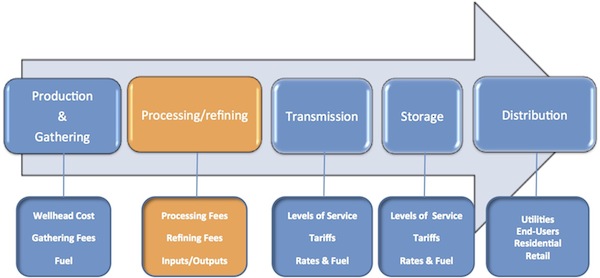
Natural gas that is going to be injected into the pipeline has to meet the pipeline specifications and has to have more than 98% methane. The second step in the logistics chain for natural gas is the processing of the produced gas. Processing is done for two main purposes: 1) removing other heavy hydrocarbons and removing the contaminations. Other extracted hydrocarbons, natural gas liquids (NGLs) and condensates are marketable and can be sold.
The first mini-lecture explains the refining and processing of natural gas. The second one focuses on the NGLs, their applications, and their market.
Key Learning Points for the Mini-Lecture: Processing and NGLs
While watching the mini-lecture, keep in mind the following key points:
- Produced natural gas has to be processed and purified to meet the natural gas pipeline specifications.
- Removing heavy hydrocarbons from natural gas has to be done to protect the burner tip from volatile fuel.
- Produced NGLs are marketable products.
- Water, sulfur content, carbon dioxide, and nitrogen have to be removed from natural gas.
- NGLs include ethane, propane, butane, pentanes, and natural gasoline.
Mini-lecture: Natural Gas Processing (9:04 minutes)
After we've gathered the natural gas from various wellheads and perhaps, brought them to a common point in a gathering system, the next thing that we want to do is kind of twofold. Number one, we want to purify the gas because the gas that goes into the pipeline system has to be about 98% methane with a lot of contaminants removed from that.
But additionally, the processing plants allow us an opportunity to extract natural gas liquids which add to the overall value chain and the actual revenue that can be derived from natural gas.
Here's just a picture of a processing plant up in Colorado. You can see, this is one of the more complex ones.
Now, the basic operations of natural gas processing plants, the first step is to remove the heavy hydrocarbons. Anything that has a specific gravity greater than methane, is considered a heavy hydrocarbon. If you think about it, the raw stream coming out of a natural gas well is going to have a lot of liquid in it. And the liquid happens to be, for the most part, these natural gas liquids. And so we can't have things like propane or butane ending up in someone's hot water heater.
Likewise, in natural gas-fired power plants, they cannot end up with any of these volatile fuels inside a boiler. They literally can have an explosion that occurs there.
And the other side of this, of course, is that we want these heavy hydrocarbons. They are marketable in the form of ethane, propane, butane, isobutane, and natural gasoline.
Simple processes with a processing plant, things like condensation. This is just, you vary the pressure and temperature of the gas stream itself, and then, you can knock out the natural gas liquids. So, for instance, when you heat something up and cool it off, liquids will drop out. If you put something under high pressure and then you reduce the pressure dramatically, liquids will also drop out of the gas stream.
Some of the towers that we'll talk about, they have oils in there which can actually absorb some of the light hydrocarbons. And those then, get funneled off. And then, fractionation is where we actually take the various liquids that may be combined and break them down into individual fractions. Thereby, forming what we call purity products, things like purity ethane or purity propane, which means the majority of that liquid is actually that hydrocarbon.
We want to purify the gas stream as well. Every natural gas pipeline company has certain standards that you can find on their website within their tariff under their statement of operating conditions. You will see that they have certain limitations on things like water, H2S, or hydrogen sulfide, which is corrosive.
Carbon dioxide and nitrogen, they simply take up space in the pipeline so they have no heating value and they just do literally waste space in the pipeline. You'd rather be pushing 98% methane than to have a higher percentage of carbon dioxide or nitrogen for that matter.
So some of the processes would be nitrogen rejection, literally, nitrogen is taken out of the gas stream.
Glycol absorption, now this is ethylene glycol. It's essentially antifreeze and it's heated up, and it can be heated up beyond the boiling point of water. So in essence, the gas stream run through a glycol absorption unit would burn the water off so you reduce the water content in the natural gas stream.
And then, also, if there's a higher level of sulfur than should be in the natural gas stream, they have what's known as an amine treater that will remove that as well.
So now we've purified the gas stream at the processing plant, essentially, we should be left with 98% methane to put into the transmission pipeline that what we call the residue point or outlet of the processing plant.
Some of the general types of processing plants. We have simple separator tower type plants, literally, the natural gas flows through the bottom. And because methane is lighter than the other heavy hydrocarbons, it will rise to the top of the column and then be basically recirculated through the plant.
Then you've got what we call bubble trays on each level and as, again, the gas flow goes through there, the heavier hydrocarbons will settle back down on these trays depending on their specific gravities. And then, again, they are piped off into tanks for storage.
As I mentioned earlier, you're going to vary pressure and temperature with reciprocating compressors. Refrigeration units and so-called re-boilers, the re-boilers are going to heat up the gas stream. Obviously, the refrigeration units are going to cool it down. And the entire time, you're pushing the gas through the processing plant using compressors. So again, raise the temperature of the gas, cool it off rapidly, we'll get condensation, and natural gas liquids will knock out of the stream.
Then we have the next step up and these are the more sophisticated processing plants-- cryogenic or what we call cryo plants. In this case, you're going to cycle the gas through refrigerants using turbine expanders. Turbine expanders in lieu of the type of compressors I was talking about that are jet engines. They're turbine engines.
Again, this idea is to cool it down. Expand the stream using a turbine compressor. And then, when you cool it down, again, you knock out natural gas liquids through the process of condensation.
The idea here, though, is to circulate this gas through the plant several times until essentially, it's been wrung out and you can extract as much NGLs as possible. It's what's called the recovery percentage of the natural gas liquids out of the gas stream.
Here's an overall schematic, and you can see here, you've got some basic-- you start at the wellhead. The oil gas separator that I had in the photo under the natural gas value chain. Condensate separator, that's the heavier liquids that are in-- they are traded in the marketplace similar to oil because they have a lot of crude oil properties.
The dehydration will knock the water out. The next tower takes out the contaminants, the hydrogen sulfide, the CO2. Nitrogen extraction will knock out the nitrogen. A de-methanizer tower literally takes the methane out. You can see when it comes off the top of the de-methanizer tower, it's dry gas. And it goes to the pipeline at the residue part of the processing plant.
And then, the final stage is what's called the fractionator. All these liquids are then broken down into their individual components-- ethane, propane, butane, isobutane, the pentanes which are C5s, and then, your natural gasolines.
And just a quick diagram here based on EIA information that shows the rise in natural gas liquids production over the last several years.
Here are some pictures of-- in the upper left-- the small processing plant and the lower right, a much larger one.
One more thing that we kind of want to talk about here regarding the processing plants is, that processing plants themselves, use some of the natural gas to run their compressors. But also, when you squeeze the natural gas liquids out, you're squeezing out hydrocarbons. You're squeezing out BTU value, heating value.
And so, the amount of gas that you put in, in terms of natural gas, is not going to be the same as what you take out in, again, in the form of natural gas, not necessarily natural gas liquids. So you can kind of see here, we call this plant volume reduction, the volume of BTUs, or the volume of natural gas that comes out on the residue side of a plant, is not the same amount that goes in on the inlet side of the gas.
Now, these are some of the ways that producers and midstream or processing companies put together their contracts. One of the most popular ones is a POP or Percent of Proceeds contract, this is a type of revenue sharing. And so what happens is, the midstream processing company goes ahead and markets the natural gas, and they find markets for the natural gas liquids. And then, they share in that revenue with the producer.
So the producer gets a percent of the net back pricing of the residual gas and the liquids sales, less whatever the midstream company's charging for their processing fees and fuel. So, for instance, we have contracts that might be a 90/10 or an 85/15. Under 90/10, the producer receives 90% of the net revenue and the midstream company receives 10%.
Now there are other producers who prefer to go ahead and market their own natural gas, and what they want then, is what's known as a keep whole agreement. That means that they want the same amount of BTUs that they gave the midstream company on the residue side. And they're going to market it so there's no revenue sharing. And they're going to pay the midstream company some fees for the actual processing.
Mini-lecture: Natural Gas Liquids (9:27 minutes)
And now, we'll talk about some of the specific products that come out, the actual natural gas liquids themselves.
These are hydrocarbon liquids derived from natural gas through the processes that we spoke about. You've got ethane which is C2H6. Propane, C3H8. Butane, C4H10. iso-Butane is an isomer of butane, IC4. The pentanes are what we call C5 pluses, that's C5H12. Natural gasolines, some of them are C5s and some are C6 through C9. And then, condensate is C6 plus. Again, condensate is a very, very light type of oil, and it is marketed in the oil markets.
Again, as we talked about, we've got to remove them from the gas stream itself because of their volatile components, but a lot of these, then, are converted into chemical feedstocks. Some are used as gasoline blending components.
The raw stream coming from most processing plants has to be processed into Y-grade. Y-grade is a composite of all the NGLs that makes it easier to ship it, either by pipeline or for trucks. Then when they arrive at a fractionation facility, that's where they're separated into so-called purity products. And a purity product would contain at least 90% composition of a single natural gas-liquid.
So, for instance, when I talked about purity propane, that would be, the liquid would be at least 90% propane.
The types of NGLs that we have, probably one of the most common ones that we do know is propane. It's approximately 40% of the overall NGL market. It is mostly used for home heating and cooking, but it is also largely used as a chemical feedstock. You can take propane and you make propylene which is a base chemical for plastics.
The primary markets for propane are the Gulf Coast petrochemical facilities. Again, the Gulf Coast is the world's largest refining and petrochemical corridor in the world.
Mont Belvieu, Texas is a large complex east of Houston. It is a huge fractionation facility. There are deliveries to and from the plant. It's a trading point. There's storage there, both above ground and underground. And there's a global market. There are actually NGLs that are exported from this area.
There is a secondary market in the midcontinent. It's in Conway, Kansas. Again, this is a much, much smaller plant than Mont Belvieu, but they have fractionation towers. There is NGL take away and delivery. There is storage there. It is a trading point. And there happens to be a petrochemical refining plant adjacent to the Conway NGL fractionation plant.
And, of course, they do have pipelines that can move southbound to Mont Belvieu so additional NGLs can make their way down to Mont Belvieu.
Ethane is about 25% of the natural gas liquids market. It is primarily used as a chemical feedstock for ethylene and propylene. Again, those are base chemicals used in the manufacture of plastics.
Now, it's rarely used as a fuel source. It can be left in the gas stream as methane. We refer to this as ethane rejection. If ethane prices are low but natural gas prices are fairly strong, then the ethane is left in the natural gas stream which raises the overall BTU content for the stream. And, of course, this is highly price dependent.
Sometimes in the middle of winter, the actual price of the natural gas on a BTU basis far exceeds that of selling the ethane in liquid form. And so you'll find processing plants go into what they call ethane rejection, that means is, they don't want the ethane. They leave it in the natural gas stream.
Same market hubs as the other NGLs, Mont Belvieu and Conway, Texas. If you hear the term E/P mix in the natural gas liquids industry, that means that it's 80% ethane and 20% propane, and that is strictly used for ethylene production.
Butane or n-butane, because now we're talking about the normal butane, 85% of the butane is used for gasoline blending. Now we talk about RVP. In the wintertime, butane is used to stabilize the RVP. RVP is the re-vapor pressure. Now it's a measurement of the ability for gasoline to vaporize at atmospheric pressure.
Any time that you are filling your car up if you see fumes coming back up out of the tank while you're filling it, that's a measure of RVP. You've got vapor there.
Several states in the United States have those vapor recovery nozzles, those plastic things that are over the gas lid. The idea is that you want to recover as much vapor as possible because number one, they do condense and they are gasoline. Number two, they are a form of pollution when they just go to the air.
We talked about the refining process. Butane is used as a cracking component when we talked about the cracking portion of a refinery process. A lot of us know about lighter fluid, meaning butane is used in lighters. It's also a propellant in aerosol sprays. It can be used for household cooking and bottled gas. And it's also a refrigerant. It is a refrigerant that can be used at the processing plants to chill the natural gas. It is also a refrigerant used in air conditioning systems in motor vehicles.
And this is iso-butane which is an isomer of butane, also known as methylpropane. It has similar uses to the butane. Gasoline blending. It's a chemical feedstock. Again, it's also used as a refrigerant in automobiles for the air conditioning systems and it's known as R600a.
And it's also known as isooctane, this is an anti-knock gasoline additive. If you've ever had the situation with knocking your car, seems like it's starting to stall and it bangs really hard and then it shuts down, this helps to stabilize the gasoline so that those things do not happen because they can be very damaging to the engine.
NGLs, the next group of natural gasolines-- C5 pluses are considered natural gasolines. You're literally able to burn those as natural gasolines. So these are also used for gasoline blending. Now they're used to stabilize the RVP mostly in the summertime. They can be used for ethylene production. They are used as industrial solvents. They're also an ethanol denaturant.
If you think about ethanol, the vast majority of ethanol is produced from corn, and it's a form of alcohol. So it literally is corn liquor. You could drink it as an alcohol. So to discourage people from doing that and to prevent the sale of it as that, basically, they have to add a little bit of natural gasoline to it so, in essence, it becomes lethal, and it certainly tastes bad.
It's used as a crude diluent, which means it can be used to dilute crude. For instance, in the Western provinces, especially in Alberta, Canada, you have the tar sands oil which is also known as bitumen, and it's extremely thick. And so they can take the natural gasolines and they can blend those, or add them to the thick crude, which makes it a bit thinner which allows it to more easily ship in the pipelines.
And again, the biggest market hub for natural gasolines is Mont Belvieu, Texas.
Pricing wise, you can see, this is just a comparison of the natural gas liquids which tend to run in sync with things like natural gasolines and crude oil.
And here, you can see just basically, again, another trend where you've got spot prices for natural gas liquids. Compared to Brent crude, Mont Belvieu propane, you can see that that's in here. And then, of course, natural gas.
Now this last slide I want to show you has to do with the fact that you can see the spike of mostly propane, this is propane spot pricing. And you can see in the winter of 2013-2014, there was a huge spike, specifically Conway, Kansas.
Now, this didn't necessarily have to do with the amount of propane, it had to do with the deliverability. We couldn't get the propane to the markets that needed it the most and that was in the Upper Midwest. You can see this past winter of 2014-2015, there was not the same type of spikes in Kansas or at Mont Belvieu.
And then lastly, I've got a slide here that kind of gives you an appreciation of the value of natural gas when you add in the revenue from the liquids. A lot of people want to know, why do producers continue to sell natural gas above or below $3? How is it possibly economical?
Well, if they're also extracting natural gasolines, then you've got a considerable amount of revenue there that's possible so you can see as you move across this spreadsheet and you get over to the liquid price per MMBTU, it is considerable.
And then we talk about the spreads that the midstream or processing companies get, and you can see in this particular sample, the total stream was worth about $3.20. The gas that it cost them to basically run the plant, was $2.65 so their crack spread becomes $0.55 per MMBTU, which is a pretty healthy spread.
Transmission Pipelines
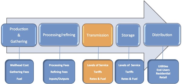
Once the raw natural gas stream has been processed, it is now “commercial grade” or “pipeline quality” natural gas. The outlet, or residue, side of the processing plant delivers the gas to the transmission pipelines. The primary function of transmission pipelines is to move the gas from the producing basins to the market areas.
The following mini-lecture will illustrate the function and operation of the transmission pipeline systems.
Key Learning Points for the Mini-Lecture: Transmission Pipelines
While watching the mini-lecture, keep in mind the following key points:
- Natural gas transmission pipelines connect supply areas throughout the country with major market areas.
- Transmission pipelines are large-diameter steel pipes.
- As opposed to gathering lines, transmission pipelines run at very high pressures.
- The US has a huge pipeline "grid" running from coast-to-coast with several pipelines connected to one another.
- Various sources of supply and consumption connect to these pipelines.
- Large compressors are used to move the gas along the pipelines.
Mini-Lecture: Natural Gas Transmission (12:00 minutes)
Moving along now, in our discussion of natural gas, the logistics and value chain. Now that we have gathered and processed the natural gas, it's ready to be shipped to market using natural gas transmission pipelines.
Now, these are going to be large diameter pipes. This is steel pipe. These days, you'll find a minimum of probably 16 inches all the way up to 42 inch pipelines. And the primary function of transmission pipelines is to connect the supply areas to the market areas.
As we mentioned, with the wellhead and using compressors to boost the pressure of the wells to meet the downstream pipeline pressure, we have to push this gas now, in a transmission pipeline from those points of receipt of the wellheads all the way to the marketplaces. And in some cases, we're talking about pipelines that originate in South Texas and run all the way up to New York City. So again, you can imagine you've got compressors all along the way continuing to boost the pressure up.
We say, that the gas flows to the point of least resistance. That just means that on the consuming end, as the gas is being burnt at the various end users then other gas has to replace it. And so the pressure is lower on that end, the higher pressure pushes that.
Here's just some pictures of the process of actually building transmission pipelines. You can see in the upper left, that's the right away that's being dug out and then all the steel pipe, steel tubing, is laid in place, in the middle picture. You can see where they're actually having to come up over a bend of a mountain there. And then these sections get welded together. And in the lower right, you can see this is specific type of equipment that lifts the pipe up once it's been welded and lays it into the trenches.
When all's said and done, this is what you see. So if you ever see pipeline right away, all you'll see are these above ground valves, everything else is buried. Now, here's a pipeline company in the state of Oklahoma. And I like to use this diagram, only because if you look you can see the red pipes or the transmission systems, and all the yellow are the spidering types of gathering lines. So you have all these various gathering lines of various wells coming to the yellow squares, which are the processing plants. And in turn, once processed and cleaned up, the gas goes to these transmission pipelines.
Terminology wise, we talk about receipts. Any source of natural gas that is received into the transmission pipeline is known as a receipt. Now, these can be wells that are flowing directly in. These can be what we call CDP's or Central Delivery Points.
Again, getting back to the diagram of the multiple wells coming to a common point and then they can come into the transmission pipelines. Processing plants, what we call the residue lines. The gas that leaves the processing plant once it's been stripped of natural gas liquids and it's been clean and now meets the quality standards of the downstream transmission pipeline. It comes in that way.
Pipeline interconnects. The pipelines criss-cross each other in a lot of places throughout the country. And that provides for one pipe to send gas to another pipe. And so any time we have that gas moving from one pipe to another, then the downstream pipe receiving the gas from the upstream pipe, that upstream pipe is then a receipt point.
And then of course, storage facilities. When we put gas in the ground for emergency or peaking purposes, when we draw it out, the gas is then received from the storage facility to the downstream transmission pipeline. And on the flip side, the deliveries, one of the most common deliveries is to a local distribution company or just your common gas company at what's known as the City-gate. And that's where the gas company receives the gas and then distributes it to its various end users.
We also have Direct-connect End-users. Power plants, fertilizer plants, and other industrial and commercial customers like that, may be tied directly to the pipeline as opposed to having a gas company serve them. And again, the flip side of what I was talking about with interconnecting pipelines, one pipeline can in fact, deliver gas to another pipeline. And then storage facilities. In order to fill a storage facility up, we have to take gas off of one pipeline and put it into the ground.
Transmission systems. Because these are-- gas is flowing 24/7, 365 days a year. The pipelines have to monitor that activity. And so this full integrated electronic system we refer to as SCADA. That is Supervisory Control and Data Acquisition. Its the electronic transmittal of pipeline data to a central monitoring and control center. They're looking at the pressures and flows. Pipeline pressures and the amount of actual volume of gas flowing throughout their system. As I mentioned, it's monitored 24 hours a day.
But the control part comes in where they actually have control of the pipeline facilities. They can start and stop compressors. They can open up and close valves. And they also can control what are known as regulators. The regulators can control the volume of the gas or the pressure of the gas on the system.
This is what a typical gas control center might look like. Again, these are manned 24/7 and they're keeping an eye on the pressures and flows throughout their system. Now, here's a simplified map of what the North American natural gas pipeline grid would look like. The sort of shaded areas represent large producing basins. And again, the idea being that transmission pipelines have initially been set up to move gas from these various supply basins to the consuming regions.
Now, here's the traditional flow. Again, coming from major basins to other areas. And you can see, traditionally pipelines were bringing gas to the Northeast, but that has changed in recent years. And the reason it's changed is because of the shale plays. Again, looking in the Northeast at the Marcellus and the Utica, there is a considerable amount of gas coming out of the Marcellus these days.
Well, if there's gas being produced right there in the Northeast, then supplies coming from other regions are being backed up. Here were some of the original projects due to move gas from, as believe it or not, as far back as the Rocky Mountains, all the way to the Northeast. And then the initial production coming from the Marcellus, get it over to the Northeast markets as well.
And now, there are, as you can see, quite a few projects. Some are trying to move the Marcellus gas still towards the east, especially New England, but others are actually going to be moving gas out of the Marcellus and Utica shales to the southeast part of the United States and back to the Western part of the United States. Here are some of the projects that are specific to the Marcellus. Again, moving gas to the east or moving gas to the southeast down the Atlantic seaboard to two, of what will be eventually LNG export facilities.
And still, New England is pretty much starved for gas. So some of the gas is trying to get over there. There are expansion projects that you see over here, in the lower right because prices in Boston and New England for natural gas in the wintertime are absolutely astronomical. And it's because they have-- they do not have a lot of access to the regional supplies. So there will be pipeline expansion projects to help alleviate this problem in the coming years.
And as I mentioned, some of Marcellus shale gas is going to move back west. They actually have a surplus. They're producing more than the Northeast is currently using. And here's just an example. This is Energy Transfer Partners out of Dallas. They've got a plant project to bring Marcellus and Utica shale gas back across to what is known as the Panhandle Eastern Pipeline Company or PEPO, to help serve their markets up in the upper mid-- excuse me, upper Michigan and over even into parts of Ontario.
Some more west bound projects. American Natural Resources or ANR is owned by TransCanada pipelines. And you can see here, they've got projects to move gas west out of the Marcellus and Utica shales as well. Here again, are some specific Northeast to Southeast pipeline projects. There are supposed to be economic growth in the southeastern part of the United States. And so there's expected increase in demand there. So some of this Marcellus gas is going to try and get in that direction.
As I mentioned before, there are two LNG import facilities along the Atlantic seaboard. One is Cove Point, Maryland and the other is Elba Island, Georgia. Now, it's highly likely that these will become natural gas export points so there are some pipeline projects in the works to get gas from the Marcellus down to those facilities.
These are just some of the key cash points. We talked about the cash marketplace before. You have seen on the natural gas intelligence website where ICE daily cash prices are posted. These are some of the key cash market points up in the Marcellus and Utica region.
Now, these are just some pictures of what can happen if the pipeline is not monitored properly. This was actually a pipeline that burst. It was the El Paso pipeline which runs from west Texas all the way to California. This unfortunately, occurred in a national park in Arizona. And it literally, as you can see, blew a crater out. At the time they took these pictures, I'm assuming these were the first people on the scene. The safety people with the pipeline company. You can see there's still methane in there that's burning.
This is the cutaway of the side part of the pipe. Now, it blew out exactly where it was welded together. There were a combination of things that had happened here. Obviously, this part of the line had not been inspected on a regular enough basis to in fact, determine there was some type of a defect in the pipe. The other thing that more than likely happened was that the pipe was overpressure. Then in fact, it was running at a much higher pressure than was safe for this particular segment.
And then there had to be some type of ignition source there because once the pressure of the pipeline erupted the pipeline, something had to ignite the natural gas, unfortunately. You can see this entire area has been scorched by the fire that came from this particular rupture.
Here's a piece of the pipe. This is part of the pipe that's missing. First of all, two things, if you look back here, you don't see any snow whatsoever. This whole scorched area within the right away and then yet, off to the side somewhere you see snow on the ground and literally pieces of the pipe that were blown over into the woods.
This is a section of pipe again, that blew out of there. Now, when the pipe is actually made it's made from sheets of steel and it's rolled. And then there is a weld that runs along laterally and that's where we get the rolled piping or the rolled steel. So you can see this explosion was enough to rip an entire section out of the ground and rip it along its initial weld.
Storage
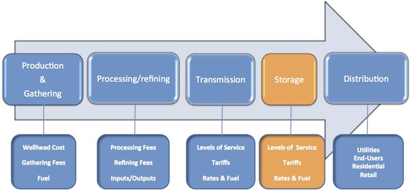
Natural gas storage facilities provide the industry with flexibility. During times of “peak” demand such as harsh winters or extremely hot summers, utilities can rely on supplies stored beneath the ground. Likewise, during times of low demand, excess supplies can be stored for when they are needed. For savvy marketers, storage capacity can be used to take advantage of the price fluctuations in the market. There are three main types of natural gas storage facilities: depleted oil & gas reservoirs, salt caverns, and aquifers.
The following lecture covers the types of natural gas storage, traditional and current uses, and the industry players who use storage capacity and why.
Key Learning Points for the Mini-Lecture: Storage
While watching the mini-lecture, keep in mind the following key points:
- Storage facilities provide "peaking" supply in times of increased need.
- Storage facilities can be used to store excess supply in periods of low demand.
- Storage facilities are largely depleted oil & gas reservoirs but can also be salt caverns and aquifers.
- LDCs have long used storage facilities for supply during extreme cold.
- Electric utilities rely on storage facilities for extra supply during peak air-conditioning loads.
- Marketers use them to provide a variety of value-added services and to take advantage of price swings.
Mini-lecture: Storage (12:32 minutes)
Now we have gathered the gas. We have processed it. We have put it in the transmission pipelines. Before we take it on to the local distribution companies and ultimate end users, there is an incremental step-- which may or may not occur-- and that is the underground storage of natural gas.
Here, again, is the energy commodity logistics and value chain. You can see that the fourth step in our process here is that of storage. Here's a cutaway of what a potential storage facility could look like. Again, it's really just, in most cases, a depleted oil and gas reservoir. So you treat it the same as you would a typical oil or gas well.
Here we have some vertical wells and one horizontal well. This is a good example of what a horizontal well looks like. You can see that by cutting across the reservoir horizontally you can extract more production than the straight, vertical holes that come down in traditional wells.
This is an above ground shot of a storage facility. You don't see the caverns. You just see what's above ground. In this particular case, there is a pipe being laid that's going to connect a power plant directly to this storage facility.
Traditional uses for storage-- mostly by local distribution companies or gas companies in the winter time, when there was high demand and there was not enough wellhead gas to meet the demand. And so gas had been stored, mostly in the summertime, and was utilized for what we refer to as peaking supply, that is when demand peaks due to unforeseen changes in the weather.
The summertime-- low demand for natural gas, because again it was mostly a winter fuel. Also, prices tended to be lower in the summer than the winter time, because of lower demand. Also, pressure relief-- as we saw in those photos as to what can happen when the pipeline pressure gets too high, when the pipeline pressure is, in fact, high, pipeline companies can put some of that gas in the ground and reduce the pressure. Also price opportunity-- when prices dip, one can buy some natural gas at those lower prices, stick it in the ground, and save it for when demand may go up and prices can be higher.
Probably, though, the number one utilization of underground storage by gas companies is for emergency deliverability. We mentioned that term deliverability in talking about the well head, the amount of gas that can be pulled out on a given day. We have seen harsh winters just two years ago, the winter of 2010, 2011, was fairly harsh. And so local distribution companies, your gas company, can rely on gas in storage to supplement the wellhead gas that they're receiving otherwise.
In the Gulf Coast region, if there is, in fact, an active hurricane that enters the Gulf, a lot of the offshore rigs are going to be evacuated and shut down. There's a substantial amount of natural gas that is then curtailed. Well, supply in underground storage facilities can supplement the loss of that natural gas deliverability.
Traditional operators and users of natural gas storage facilities-- mainly the pipeline companies in both the supply and market areas, and then local distribution companies in the market areas themselves.
Types of natural gas storage-- there are mainly three types. Depleted oil and gas reservoirs being the most common. Why? Because you're taking what used to be an oil or gas well, and you're now going to put natural gas down in it. So we already know the characteristics of the wells. We know how much natural gas they can hold.
There are also terms, permeability and porosity. These are geologic terms. The permeability is how much natural gas can actually be held in the formation. And then the porosity, the types of little pores in the formation itself as well. Those two combined can give us a determination of the deliverability of that particular reservoir. That would allow us to determine whether it would make a good storage facility or not.
We can inject gas from the transmission pipeline. If the pressure's high enough, the gas will freely flow into the formation. As we add natural gas to the formation, and the pressure increases, we may actually need to use compression to draw the gas from the transmission pipeline, and shove it down into the reservoir.
Conversely, when it's time to utilize the gas, we can withdraw it. If the pressure is high enough, that is if it's higher than the downstream transmission pipeline, it'll free flow. At such point in time, as the reservoir pressure meets or is less than the downstream transmission pipeline, we'll use compressors to boost the pressure up from the reservoir.
Oil and gas reservoirs converted to storage take approximately 50% of the capacity to be filled first before they can utilize it. We refer to this as the cushion, or base, gas. So, for example, a one billion cubic foot natural gas reservoir that we would like to convert to storage is going to take 500 million cubic feet of natural gas to be put in place first. The tier above that is what we refer to as the working gas. It is the usable space. It is the recoverable gas. This factor itself is one of the reasons why developing storage facilities can be so expensive -- because that initial 50% of natural gas will have to be purchased and cannot be sold until the end of the life of the storage facility when it's extracted.
Another type, and these are very much used along the Gulf Coast, are salt domes, or salt caverns. There is literally a large, impermeable hole. When the natural gas, or natural gas liquids, are put into salt caverns, they do not escape. If you find a salt formation, it's very easy to form one of these.
High pressure water carves out the reservoir. Then you inject gas into the cavern. And free flow it in or compress it, just as you will with the oil and gas reservoirs. The converse process of withdrawing, again, can also be free flow or compression. These actually have very high deliverability. They can be cycled numerous times. That means gas can be injected one day, withdrawn the next day, and so on. And so they make a very, very worthwhile type of storage facility.
Aquifers, these are water formations that are utilized for storage. You generally see these only in the upper-Midwest market areas, where they are used for emergency supply. You're pushing gas into the aquifer, the water comes out. When you need the natural gas, you push water back in and take the gas out.
Now, these are the least desirable types of storage facilities. There's a high development cost because there is no pre-existing facility in place. The aquifer reservoir characteristics are literally unknown. The boundaries of an oil & gas reservoir, or the boundaries of a salt cavern, can be determined, but not an aquifer.
The base gas requirements-- we talked about an oil & gas reservoir requiring about 50% of base gas. In the case of an aquifer, you need 90% base gas to hold back the water. So you only have about 10% of capacity that you can utilize. And then you're going to have to use gas compression to force the gas into the aquifer, or water injection, when you wish to remove the gas.
We have a couple of classifications of storage. We have what we call seasonal, and these are mostly the depleted oil and gas reservoirs. We inject gas in what is normally the lower demand, lower price period of April through October. And then we withdraw the gas in what we refer to as the winter months of November through March.
Now, these time-frames are very key to the industry. Pricing for natural gas, when we talk about seasonal pricing, we use the terminology summer and winter. They are not the typical summer and winter periods that we're accustomed to. There are no four seasons within the natural gas marketplace. We talk about summer being April through October because it corresponds to the injection period for natural gas storage. And we talk about the winter as being November through March, because it is the typical withdrawal period for natural gas storage.
High deliverability classification of storage are your salt caverns and your enhanced depleted oil and gas reservoirs. Has there been additional compression added to the oil and gas reservoir storage facility? Do we have horizontal wells? Both of those will increase the deliverability of the oil and gas reservoir. Salt caverns by themselves have high deliverability characteristics.
Current users-- we see pipelines still using these to provide what we refer to as market-responsive services. Seasonal storage, as well as cyclable storage-- cyclable storage meaning that you can inject or withdraw at any point in time during the term of the contract that you have with the pipeline and their storage affiliate. Park and loans-- this is a short-term service that pipelines can provide. If you have excess gas, they allow you to store it in their facility for a short period of time. If you find yourself short of supply relative to demand, you can also borrow some gas from the pipeline for a certain fee. But you will actually give them the molecules back upon the repayment time.
Local distribution companies, again your gas companies-- traditional storage usage. They're going to use the storage for short-term peaking of services. These days, however, what they pay for storage is going to be regulated by the respective public utility commission in the state where the LDC operates.
The largest group of current users are your marketing and trading companies. We will talk briefly later on about the deregulation of the industry. But there are third-party marketing and trading companies that are now providing services that were once provided by the pipelines and LDC's. We call this the re-bundling of those services. So they can provide peaking gas. They now provide same-day gas. That is, if the utility or end-user needs gas today, for some reason, because they have storage capacity they can sell them gas today.
In other situations, they can provide gas on demand. A marketing and trading company with cyclable storage can literally allow an electric utility, for example, to draw gas from them as they need it. Each one of these services commands a premium. And this is really where marketing and trading companies make their money on these added value services. They cannot provide these added value services, however, without storage.
Storage facilities also allow them to respond to changes at the markets. Price volatility, that is the movement of price up and down, as well as the speed at which price changes occur. Those represent opportunities for savvy marketers to buy and sell. And they can do this because they have storage facilities that will allow them to store the gas when prices are lower, and to sell gas when prices are higher, both in the physical cash market, as well as in the financial market on the New York Mercantile Exchange, which we will talk about in both lessons seven and eight.
Distribution and Liquified Natural Gas (LNG)
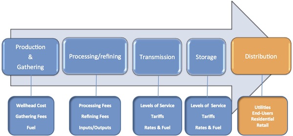
The final step in the logistics chain for natural gas is delivered to the burner tip. This can be accomplished by Local Distribution Companies (“gas companies”), or pipelines can deliver gas directly to connected end-users. We generally classify the end-users as utility, residential, commercial, and industrial.
The following lecture explains the function of Local Distribution Companies (LDCs) and presents various other natural gas end-user groups.
Key Learning Points for the Mini-Lecture: End-Users
While watching the mini-lecture, keep in mind the following key points:
- Local Distribution Companies (LDCs) are gas utilities.
- LDCs lower the pressure of the gas coming from the transmission pipelines and distribute it to end-users.
- Electricity is produced by both public (utilities) and private companies.
- Generation can be simple-cycle, combined cycle, or co-generation.
- Natural gas is used in various commercial, residential, and industrial applications.
- The use of Natural Gas Vehicles (NGVs) is growing.
Mini-lecture: Natural Gas End Users (8:35 minutes)
Now we finally reach the actual end of our logistical path for natural gas from well head to burner tip. We're going to talk about the various types of end users. This is not an all-inclusive list. But we'll cover quite a few of them.
We've got basically local distribution companies which I've referred to thus far as gas companies, that's what they are, and then the various direct end users of natural gas. Local Distribution Companies, otherwise in the business known as LDCs, these are your gas companies. Whoever your local gas company is an LDC. They're going to distribute the gas to the various end users that are connected to their systems.
Their primary operation is to distribute low-pressure gas. When we talked about transmission pipelines, they move the gas at very, very high pressures. And you can't have that type of pressure coming into your house, especially into something like a hot water heater. So, they lower the pressure. You can see here, mainline transmission pipelines can be running 500 pounds per square inch to as much as 1,500 pounds per square inch. Well, the gas flow into your house at the meter needs to be cut down to four to six ounces per square inch. So, we have residential customers, commercial customers, industrial, and electric customers.
Another type of operation, they can actually perform a transportation service. In other words, several states across the country have what's known as a deregulated natural gas industry. And that includes deregulation of the local distribution companies. So, if you're a large enough end user, you actually can buy gas from an entity other than the natural gas company, your local gas company. But they still make sure that it gets delivered to you, and so they charge you a transportation fee.
So, we refer to this as transportation behind the city gate. That means within the distribution territory. So end users can have their own transportation on the LDC system. It's an open access system. So in other words, any entity that qualifies under their regulations to do so can, in fact, buy from someone else and have it transported.
Here's kind of a breakdown of that delivered price. When you get that gas bill and you look at it, these are the components. You've got the commodity is only 34% of that. So the price of the commodity itself. The LDC or the pipeline company is about 19% there of the cost has to do with the transmission pipeline transportation and storage. But then the distribution costs are 47%. So this is your gas company providing that service.
Here's just a typical residential meter. And here, we just have a large metropolitan area. This happens to be Denver. So we're going to address the actual end users. You can just see here some of the end users. Electric power is the largest end user for natural gas, 31%, followed by industrials and then residential. Commercials having a very small percentage as well. And one thing here, notice the vehicle fuel at this point in time, as of 2013, was less than 1% of the consumption of natural gas in the US.
We'll talk about electric generators. There are two different groups. You've got the electric utility generators. These are regulated producers of electricity. They're either federally regulated or regulated by the respective states. And then you have the non-utility electric generators, the so-called independent power producers. These are also known as merchant power companies.
And then, another group is known as the co-generators. These are companies whose plants actually produce electricity and steam-- steam as an actual commercial commodity. It can be shipped by pipeline to nearby facilities such as food processing or actual crude oil refineries.
Within electric generation, we have different types of generators themselves. A simple cycle generator has gas turbines. These are essentially jet engines. They're internal combustion. They use natural gas as a fuel. And then there's also steam turbines where the natural gas goes into a boiler first and creates steam. And the steam is used to push the turbines. It's not the fuel source. It's literally spinning the turbines.
You also have combined cycle plants. This is where you have a combination of gas and steam turbines. The gas turbine, again, is strictly using natural gas as a fuel. But it has exhaust heat. That exhaust heat then is pumped into a boiler where we create steam which then drives a steam turbine. So a combined cycle natural gas plants are among your most efficient. And then again we have the co-generation facilities where they've got a gas turbine which is going to create electricity. But then they also have a steam boiler where are they going to create the steam, as I mentioned, to sell as an actual commercial commodity.
And then, you can see, this is somewhat of a simplified diagram of the process itself. Now, you see on the left you have an energy supply or fuel. Now, the fuel, in this case, doesn't matter. It can be coal. It can be wood. It can be natural gas. It can be nuclear fission. It's anything that can create heat because the idea here is to take water and basically bring it to a boiling point where you have steam.
Now the steam actually drives the turbine. That's the little blue and white area in the middle part of the diagram in the center there. That turbine spins. And on the axle of that turbine are magnets, very large magnets. And they spin within a copper wire field. The magnets are of opposite polarity. And when they spin they actually create current, which as you can see, goes on out into the transmission lines. And most plants re-circulate then the steam. They cool it down. That's what those large cooling towers are that you see. And then, they recycle as much of that water as they can.
Here's what a typical gas turbine looks like. Again, you can see it's got fins on it like a jet engine. Other end users such as industrial end users, you've got petrochemical refining as I mentioned. They're going to have feedstocks created from natural gas, paper production, metals especially things like steel mills use a considerable amount of gas in their furnaces. Stone, essentially cement plants, they have components like clay and glass and silica and sand. And they actually, in addition to having furnaces, once the cement is created it's in a wet mixture, and they use natural gas to actually dry it. All types of food processing, I'm sure that everyone can come up with to use that, and then in fertilizer. Anhydrous ammonia or fertilizer, 80% of that feedstock happens to be natural gas.
Then we also have commercial uses. Believe it or not, there are large air conditioning units at, let's say for instance, in large warehouses or factories that can run off of natural gas, you know, food service, motels, hotels, healthcare, various hospitals, office buildings, and then at the retail level. And then, last but not least, we have natural gas vehicles. The market for natural gas vehicles has grown the last few years. But it's probably going to decline because just recently Honda Motors said they're going to phase out the manufacture of their CNG Civic which has been around for probably 20 years, and then also their Honda Accord CNG vehicle as well.
Now the better ones are dual fuel. You can use gasoline or CNG. But CNG still has an important usage within what we would call fleet vehicles. For instance, metropolitan buses, trucks using on short haul routes like the USPS or FedEx or UPS, and then pool cars. Various companies who have let's say a certain district and they don't need the longer range of cars, they can use CNG. But again the limitations are the limited range and refueling. Now the refueling infrastructure across the United States is getting better. But for most people, it is still a sticking point in terms of buying these types of vehicles.
Mini-Lecture: Liquefied Natural Gas (8:18 minutes)
Here's just pictures of four of the existing LNG import facilities that we have in the United States. And you can actually see there's one off of Massachusetts, one off of Georgia, one off of Maryland, and one of three that we have in the Gulf Coast region. Now, what is liquefied natural gas? It's natural gas that's cooled to a -320 degrees Fahrenheit. Now what this does is it reduces the volume by over 600 times, which makes it easier to transport and store.
So in other words, let's just say if we had a cubic foot of natural gas, there's a certain amount Btu within that. But the same cubic foot of liquefied natural gas would have 600 times the heating value. So you can see where storing the liquid or transporting the liquid, you are actually storing and transporting at a much, much higher heating value than with pure methane. So you can see here a ton of liquefied natural gas is equivalent to 47 MMbtu, or 47 million Btu. And one ocean-going LNG tanker can hold the equivalent of 3.0 Bcf of natural gas.
Pricing around the world varies from region to region. In Japan, they price LNG landed off of the price of crude oil that's imported, the so-called "Japanese Cocktail." What it amounts to is just the average price for the crude oil that's been purchased as cleared through their customs. And so really it's Japanese cleared customs crude pricing, but it's just referred to as the "Japanese Cocktail." In Korea and Taiwan, again, it's the price of LNG landed is tied to the Btu-equivalent "basket" of crude oil postings. In the UK, continental Europe, and Southeast Asia, it's a combination of oil and coal prices. again, converted to a Btu basis. And then the pricing for LNG on a Btu basis is equivalent.
Now in the United States and Canada, we have been traditional importers, and we have very limited export facilities. But we have a competitive natural gas marketplace. As you all know from your studying in earlier lessons, we have the New York Mercantile Exchange. So we have an open, active competitive marketplace for natural gas. Now Russia, China, and the Middle East, they regulate the price-- the various countries, the governments do. And they actually subsidize the price for their citizens. You can see here that because of the growth in the shale gas, we have steadily declined our imports over the years.
Now the US as an exporter, some of the reasons it makes sense for us, we do have a surplus gas supply. The shale plays and the tight formations have resulted in abundant, relatively cheap supply of natural gas. $3 or less is an extremely cheap price for natural gas. And the EIA estimates that we are producing about 3.0 Bcf a day more supply than we have market for.
And as I mentioned in the previous slide, we have a competitive natural gas-based pricing market. This is actually causing some renegotiations of some of the existing global contracts. In other words, Japan sees the coming of LNG exports by the United States. And so they're already talking to some of their suppliers and saying, you know, look, we want to get off of this crude oil pricing type of mechanism in our contracts and convert over to some type of natural gas index.
We have existing LNG import facilities-- those pictures I showed you in the beginning. And we actually, believe it or not, we are exporting virtually at the moment. Since we no longer need natural gas imports in the form of LNG, what's happening is those entities in the United States who have contracted for tanker loads are literally selling them mid-sea, so to speak, sending them to different ports rather than coming to the United States. And then we actually have had, for about 20 years, a small LNG export facility off the coast of Alaska at a point called Kenai, and that's been operated by Conoco Phillips.
You can see here now the red squares represent existing LNG points-- again, off of Massachusetts, Cove Point, Maryland, Elba Island, Georgia, and then we have about four in the Gulf Coast area. Now these are going to be the logical facilities to export. They have about 60% to 70% of the infrastructure in place already. They can handle tankers for offloading. They have onshore storage. They have connections with pipeline companies.
So what they're doing, is they are building the liquefaction trains. We talked about the fact that the natural gas has to be supercooled. Well that takes a liquefaction facility or train to be built. So in other words, they've got a lot of the infrastructure already in place. So some of these other companies that believe they're going to dive into this particular arena are not going to have the facilities. It's going to cost them a considerable amount more investment.
You can see here, of course, the natural gas exports and re-exports by country. Again, we have declined in terms of our imports. And then all of a sudden, you can see we've actually started to do some exporting. And then the ways that it gets to market. Again, this is that logistics and value chain we talk about for natural gas. In the case of exporting LNG, you can see here that the wellhead gas is going to move by pipeline to the liquefaction facility. And then it gets shipped to a particular port of entry where it's regasified and then distributed to the various areas of need. So it's sort of the opposite process that we've been used to for decades now, where we actually receive the LNG, and we regasify it and we utilize it through the pipeline systems of the various end users.
Pricing wise, again, here in the United States, we've got a financial natural gas forward market, which you're familiar with is the NYMEX. It provides price discovery. so everyone knows what the price is. Now just currently based on the one-year average price for natural gas at Henry Hub, it's approximately $3.05 at the time that I put this particular lecture together.
Now these are the estimated supply chain costs in US dollars per MMBtu. Approximately $2.15 represents the process for the liquefaction. Shipping overseas is about $1.25. Regasification at the new port of entry is approximately $0.70 per MMBtu. So you have total costs of about $4.10. So in this particular situation, you're really around $7.15. And I apologize this still says $7.05 on it.
Now when we compare that to world pricing, you can see that there are not that many places in which current LNG exporters can make money at $7.15. Now throughout Asia, that's still a pretty good deal. And they're still going to make money in parts of South America. But over in Europe, you could not at the present time export LNG and make money over there.
Now this situation has dramatically changed. One of the events that created impetus for the US to consider exporting LNG had to be back in March of 2011 with the Fukushima nuclear power plant disaster in Japan. As I mentioned earlier, Japan is solely dependent on imports for natural gas and imports in the form of LNG. Well at the time, they shut down all of their nuclear power plants. So the demand for natural gas in Japan spiked, and we were seeing prices upwards of $14 per MMBtu. So you can imagine at the time those planning the LNG export facilities out of the United States were expecting extremely lucrative business and very, very large profit margins. Such is not the case today. And in fact, Japan is looking at relicensing their nuclear power plants again.
Optional Materials
Liquefied Natural Gas Video by Student Energy (2:24 minutes)
LNG, Liquefied Natural Gas. LNG is natural gas that has been cooled to at least minus 162 degrees Celsius to transform the gas into a liquid for transportation purposes.
To understand why liquefying natural gas is important, we first need to understand natural gas's physical properties. Methane has a very low density and is therefore costly to transport and store. When natural gas is liquefied, it occupies 600 times less space than as a gas.
Normal gas pipelines can be used to transport gas on land or for short ocean crossings. However, long distances and overseas transport of natural gas via pipeline is not economically feasible. Liquefying natural gas makes it possible to transport gas where pipelines cannot be built, for example, across the ocean.
The four main elements of the LNG value chain are, one, exploration and production, two, liquefaction, three, shipping, four, storage and regasification. At the receiving terminal, LNG is unloaded and stored before being regasified and transported by pipe to the end users.
The demand for LNG is rising in markets with limited domestic gas production or pipeline imports. This increase is primarily from growing Asian economies, particularly driven by their desire for cleaner fuels and by the shutdown of nuclear power plants.
The largest producer of LNG in the world is Qatar with a liquefaction capacity in 2013 of roughly one-quarter of the global LNG production. Japan has always been the largest importer of LNG and in 2013 consumed over 37% of global LNG trade.
The extraction process also has environmental and social issues to consider. LNG projects require large energy imports for liquefaction and regasification and therefore have associated greenhouse gas emissions.
Spills pose concerns to local communities. There have been two accidents connected to LNG. But in general, liquefaction, LNG shipping, storage, and regasification have proven to be safe. LNG projects require large upfront capital investments, which can be a challenge in moving projects ahead.
That's LNG.
World LNG Estimated Landed Prices: Jan-18 Diagram
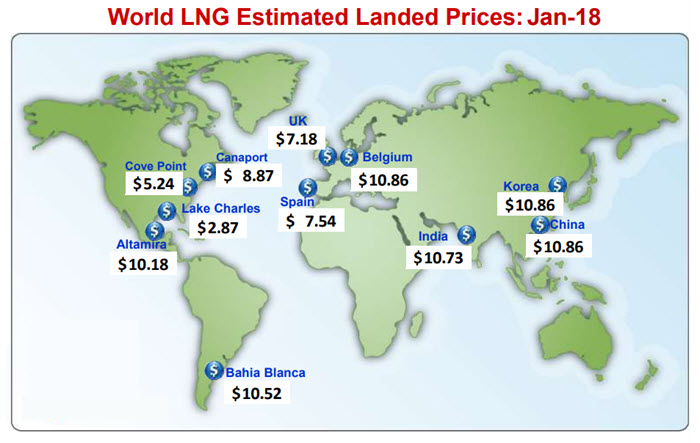
| Country | Price, $US/MMBtu |
|---|---|
| Cove Point | $5.24 |
| Altamira | $10.18 |
| Lake Charles | $2.87 |
| Bahia Blanca | $10.52 |
| Canaport | $8.87 |
| UK | $7.18 |
| Belgium | $10.86 |
| Spain | $7.54 |
| India | $10.73 |
| Korea | $10.86 |
| China | $10.86 |
Natural Gas Regulation & Rates
Key Learning Points for the Mini-Lecture: Natural Gas Regulation & Rates
While watching the mini-lecture, keep in mind the following key points:
- All interstate natural gas pipelines are regulated by the Federal Energy Regulatory Commission.
- Prior to 1985, pipelines and gas companies were the sole providers of gas supply. They bought the gas, transported it, and sold it.
- Deregulation later “unbundled” pipeline services, leading to the “spot” market and the emergence of marketing companies to take-on this role.
- Interstate pipeline companies provide different levels of service including firm and interruptible transportation and storage.
- Interstate pipeline companies must file a “tariff” of rates and services with FERC and the rates must be “just and reasonable.”
- Safety issues – all pipelines are regulated by the Department of Transportation.
- Pipelines must post all tariff information on a website.
Mini-lecture: Transportation Regulations and Rates (14:57 minutes)
In this lesson, we're going to talk about another piece of the value chain for natural gas from wellhead to burner tip. And that's the actual transportation rates that transmission pipelines charge for service, and, again, we're talking about moving gas from point A to point B. And we need to talk a little bit about the regulations that form the background for this particular service and for the regulation of the pipelines.
In 1938, there was what was known as the Natural Gas Act. This is still an important piece of legislation today because when you see the lesson on the exportation of LNG from United States, you'll see in there that projects of that nature still have to be approved under the Natural Gas Act of 1938. They have to receive what's known as a 7(c) certificate for the actual construction, and that is issued by the Federal Energy Regulatory Commission.
Now, under the NGA of 1938, both local distribution companies and pipeline companies were given a utility status, because back then we had what was known as a bundled service. The pipeline companies themselves were actually buying the natural gas, transporting it, and selling it to the end users connected to their pipes. Now the NGA utility status gave the pipelines a few things.
Number one, they had a protected territory so no one could duplicate the exact route or service territory that the LDC or pipeline was going to serve. However, in return for that, they had to act "in the public interest." They had to file what were deemed to be "just and reasonable" rates of service.
Now, one of the benefits then of being the utility is that they actually obtain the right of "eminent domain." So, they can actually condemn a land owner's property if they believe that that particular route is necessary for their right of way. And as I mentioned just a few seconds ago, they provided "bundled" services. In other words, they bought, transported, stored, and sold the natural gas, and they had no competition on their particular pipeline.
Under the Natural Gas Policy Act of 1978, the Federal Energy Regulatory Commission was established. It replaced the former Federal Power Commission. Now, in '78, the Carter Administration actually believed, or there had been a study done by the Department of Energy where, in essence, the United States would run out of natural gas by the year 2000. So, to encourage the exploration and production of new sources of natural gas, they set minimum price controls on natural gas. They literally started with a certain price, and it would escalate monthly automatically without any consideration for basic supply and demand fundamentals.
So, this is what led to this big gas "bubble" that we had in the early '80s. As we've seen over the last few decades, prices tend to go up and tend to go down, and we've had these situations where we've had bubbles, and then the bubble bursts. So, in the early '80s, the natural gas industry took a big hit because prices fell dramatically.
Now, in January 1985, those price controls finally expired. Natural gas was now going to be bought and sold in a more competitive environment, and things like supply and demand were going to be taken into consideration. The pipelines, though, had to give up this merchant function. That means they could not be the only exclusive sellers of natural gas anymore, and these excess supplies that we had in the '80s, they led to the need for entities to market those supplies that the pipeline still had under contract.
And so, in some cases, the pipelines themselves formed what were called affiliated marketing companies, but this also-- this January 1985 expiration-- these prices led to what we call today, the "spot" market for natural gas. That is, not so many longer term contracts as had been the case before, and so a lot of marketing companies jumped into the game. These were non-pipeline affiliated ones. And so, they went ahead and decided to go out and purchase this excess gas that was on the market from the producers and turn around and find end users for them, thus duplicating what the pipelines had done for decades.
Again, as I mentioned, this was the evolution of the "spot" market itself. FERC issued Order #436. Now this is known as the "Open Access" rule. What that did was that basically dictated to the pipelines that they were going to have to offer their transportation services to anyone who was interested in it on a nondiscriminatory basis. They also had to file various levels of services that they were going to provide, as well as the rates they were going to charge.
They had to establish what were known as nomination and allocation procedures. Now, nominations are merely a schedule that you as a shipper provide to the pipeline company that lists the supply sources that you have coming into their pipelines. These can be wellheads. They can be processing plants. And then, you also tell them where you want the gas delivered, thereby establishing what we would call a path, a transportation path.
In FERC Order #497, because I had mentioned earlier, some of the pipeline companies went ahead and immediately formed their own marketing groups after 1985 to take advantage of the surplus supplies. But the federal government was, once again, concerned about a potential monopoly, and pipelines were giving capacity to their marketing companies, so this basically prohibited that. The interstate pipeline companies had to separate from their affiliated marketing companies and could no longer offer them any type of private or preferential deals.
Now, the types of services that natural gas transmission pipelines provide today, the first one, in terms of just actual transportation service, is what's known as FIRM, or what we call FT FIRM transportation. Now, what happens here is the shipper pays what we call a Demand Fee or a Reservation Fee. Now, they pay this once a month to reserve a certain amount of quantity in the pipeline. We call that the Maximum Daily Quantity. Now, that's reserved, and the shipper pays for that regardless of whether or not they actually use it.
And then, as they use it, the pipeline measures the actual natural gas that's coming into their pipe and being delivered on behalf of the shipper, and they charge what's known as a Commodity Fee or a Usage Fee. So, at the end of the month, the pipeline has measured the amount of gas the shipper flowed through the system, and they will charge them an additional fee. Pipelines have what are known as minimum and maximum transportation rates that they file with the Federal Energy Regulatory Commission, but they also have the right to sell unused capacity. Any time a FIRM shipper or a shipper who has FIRM transportation does not use 100% of their contracted space, they can actually sublease that, so to speak, to interested parties.
Now, within the FIRM transportation contract that you have with the pipeline, you'll have what's known as a Path. In other words, you will have the right to move gas from the points of receipt that you have, whether they're wellheads, processing plant outlets. You may have gas and storage that you want to bring into the pipeline. So they will give you a Path that will allow you to bring those receipts in and set them to certain delivery points that you have, and, again, this is known as your Primary Path. This is your right. This is what you've got reserved.
And then, sometimes, what they'll do is they'll allow you a Secondary Path. If there are not others using the space, then you may be able to go ahead and use that as rights under your FIRM contract.
Now, another service that they offer is, if the pipeline hasn't sold all of their capacity on a FIRM basis, they'll have what's known as INTERRUPTIBLE space. Now I put this in all caps on purpose, because you have to realize that what's going to happen is if they have extra space and you take it on an INTERRUPTIBLE basis, yes, you're going to get a discounted rate because they want to go ahead and use that space, but it's INTERRUPTIBLE. In other words, it is subject to recall by the pipeline at any time. And so, if you have a situation where you're making a FIRM gas sale to an end user, or you've promised the producer that you're going to take their gas, you do not want to enter into INTERRUPTIBLE transportation. And, again, since it's INTERRUPTIBLE, you're not paying any type of Reservation or Demand Fee. You are strictly paying the Commodity Fee.
One of the pipelines that I like to use in this course, because I believe it's pretty simplistic the way they're set up, is Natural Gas Pipeline Company of America. Now they are a subsidiary of Kinder Morgan out of Houston, but you can see here they have zones. These are-- we would call-- sometimes we call these Postage Rate Zones, but the zonal rate matrix makes it very simple to determine what the rate is going to be.
For instance, we're going to deal with the Midcontinent Receipt and Delivery Zone. And so, you can see, that's sort of in parts of Kansas and Oklahoma, primarily. And so we're going to be dealing with the idea that we're bringing gas or our receipts are in this zone, and then we're going to deliver them to Chicago.
Now, if you look up over near Lake Michigan, where Chicago is, you see it's the Iowa-Illinois Receipt Zone. That's also known as their Market Zone. So, we're going to talk about moving gas from Oklahoma in this Midcontinent Receipt and Delivery Zone, up to the Market Zone, which is known as the Iowa-Illinois Receipt Zone.
Now, when you go to NGPL's website and you look up their tariff, under the tariff, it says, Currently Effective Rate Schedule. And so, these are the rates that they currently charge to move gas from some points that you see on the previous map to another point on the map. Now, we're going to be dealing with the Midcontinent area, so if you look at the Receipt Zone, which is the left column, and you go down 1, 2, 3, 4 categories, OK, you will see there that the Reservation Fee to move gas from the Midcontinent Zone to the Market Zone, which is the top of that column where the rates are, the Reservation Fee is $9.18. That's per month. You pay that up front for the space that you want reserved, and then, when you actually flow the gas, when they meter it at the end of the month, you're paying about a penny and a half for the Commodity Fee.
One of the things that occurs in terms of the cost of moving gas is that of fuel. So far, our costs are the Reservation Fee, a Commodity Fee. And now what happens is, when the gas moves from point A to point B, we've talked before in terms of a logistics chain about this idea that they're using compressors along the way.
Now, compressors, for the most part, are going to be natural gas. They may have some electric compressors, but they have the right to charge you for that. They can charge you for the cost of the electricity to run the compressors, or they can-- what they do is they'll deduct the fuel that they use along that path.
Additionally, when there's some type of a maintenance or some type of operation where they actually have to vent the natural gas pipeline, they get to account for that, and the shippers have to make that up to them. And so, the way it's done is they withhold a certain percentage per path. So, for instance, in the case of our example, whatever the fuel deduction is to move gas from Oklahoma, the Midcontinent Region, to Chicago, the Iowa-Illinois Market Region, they have that in their tariff, and they will retain that much natural gas from you. So, we use terms like "Lost and Unaccounted for" because this is gas that, again, has been vented or, perhaps in some cases, has even leaked from the pipeline, and they really cannot quantify it exactly, but they also have what I mentioned is in terms of compressor fuel.
Now, further down in the NGPL tariff, you will see these fuel percentages. These are the charges of fuel that they have the right to retain. Now, again, getting back to our example, if you look under the Receipt Zone and you find the Midcontinent, and then you move over to the right, that's under the market, what they're saying is it costs them essentially 3.2% fuel to move the gas from Oklahoma to Chicago. In other words, their estimate is that they lose that much.
So, for our purposes, what happens is, let's say, for instance, you want to move 100,000 MMBtu's a day to Chicago. If you put 100,000 MMBtu's a day in Oklahoma, essentially you're only going to get about 997,000 delivered to Chicago because they're going to retain this 3.2%. The reason we need to know that is that is a cost. So, for instance, if we are buying 100,000 in Oklahoma, we're only going to be able to sell the 997,000 in Chicago. So we have to, in terms of our economics, we have to price that in.
Now here is just another pipeline that you can see with zonal rates. This is a pipeline company called Enable, and as you can see, they're all over Oklahoma and over Arkansas and parts of Louisiana. The reason I want to use them is because here is essentially their storage rates, so we can talk about storage. It's set up fairly similarly.
You can see here FSS, or Firm Storage Service, the Deliverability Fee. That's actually similar to the Firm Reservation Fee on a pipeline. You have to pay this to guarantee that, in fact, the gas can get to and from the facility when you need it. The Capacity Fee itself, this is the charge on the total capacity that you are asking to be reserved in their storage facility.
So, let's just say you want a bcf of space in their storage facility. They're going to charge you this 2.3 cents per month for that, and then the actual monthly storage fee is going to be about a penny and a half. And then, you see, they also have an INTERRUPTIBLE Storage Service as well.
So, this basically covers the transportation rates and storage rates, which, again, are part of the value chain, and we have to take those into consideration when we are actually transacting natural gas deals, either with the producer or with an end user. So, we know either what charges to add up from the wellhead forward to charge the end user, or if we have a price from the end user, all the costs to deduct going back to where then we have what we would call a netback price at the wellhead.
Summary and Final Tasks
Key Learning Points: Lesson 6
- Natural gas travels through several stages from “wellhead-to-burner tip.”
- Wells must be connected to pipelines and/or processing plants.
- The raw wellhead natural gas must be purified and heavy hydrocarbons must be removed.
- Processing plants produce needed natural gas liquids (NGLs) such as ethane, propane, butane, iso-butane, and natural gasoline.
- Transmission pipelines are large-diameter pipes that carry gas from the producing areas to the market areas.
- Storage facilities provide extra supply in times of high demand and a place to store excess gas in times of low demand.
- End-users can vary from utilities to houses to commercial and industrial facilities.
- LNG provides 600 times the amount of energy as an equivalent amount of natural gas.
- The abundant shale gas in the US has led producers to find new markets in the form of LNG exports.
All pipelines are regulated by the Federal Energy Regulatory Commission, which has rules for how they conduct business. The services that pipelines provide and the rates they charge must be posted on their websites. These requirements came about after years of heavy regulation, which eventually led to de-regulation of the industry and a more competitive environment.
Reminder - Complete all of the lesson tasks!
You have reached the end of this lesson. Double-check the list of requirements on the first page of this lesson to make sure you have completed all of the activities listed there before beginning the next lesson.
Lesson 7 - Basic Energy Risk “Hedging” using Financial Derivatives
Lesson 7 Introduction
Overview
We've learned that NYMEX energy contracts represent the actual right to buy or sell energy commodities. So, for the commercial market participants, these provide both a market for production and a source of supply. For instance, producers of natural gas, crude oil, or refined products such as heating oil and gasoline, can sell financial contracts, thus guaranteeing that they will have a firm market in the future at a fixed price. Conversely, consumers of these same products can buy contracts to ensure that they will have a firm supply source in the future at a set price. Utilizing financial contracts to reduce price and/or commodity risk is known as "hedging." In this lesson, we will discover the ways in which commercial players in the energy industry use the financial markets for hedging their risks.
Key Learning Points – Energy Risk Hedging
- Producers and consumers of energy can reduce both their physical (market or supply) and price risk using financial derivatives such as futures and forwards.
- Futures are exchange-traded contracts such as the NYMEX energy commodities: crude, natural gas, heating oil and unleaded gasoline.
- “Over-the-counter,” or “OTC” contracts, are known as “forwards.” These are non-exchange traded and can either involve an electronic trading platform or “voice” broker.
- Hedgers are not speculators.
- In a hedge, commercial participants in financial markets take the opposite position from what they have in the physical markets.
- Financial positions must be settled monthly.
- Storage capacity can be hedged through buying one month and selling a future month.
Learning Outcomes
At the successful completion of this lesson, students should be able to:
- explain how price risk reduction can occur through the use of basic financial derivatives like NYMEX contracts and “basis swaps”;
- describe how commodity risk can be reduced;
- demonstrate a simple “hedge” structure for:
- energy commodity producers;
- energy commodity consumers;
- storage.
What is due for this lesson?
This lesson will take us one week to complete. The following items will be due Sunday at 11:59 p.m. Eastern Time.
- Lesson 7 Quiz
- Lesson 7 activities as assigned in Canvas
Questions?
If you have any questions, please post them to our General Course Questions discussion forum (not email), located under Modules in Canvas. The TA and I will check that discussion forum daily to respond. While you are there, feel free to post your own responses if you, too, are able to help out a classmate.
Reading Assignment: Lesson 7
Reading Assignment:
Seng - Chapter 6
Errera & Brown - Chapter 5
This text is available to registered students [112] via the Penn State Library.
Key Points of Emphasis
- Hedging reduces both physical and financial risk.
- Hedging is performed by commercial entities; it is not "trading."
- Hedgers have two positions, one in financial and one in physical.
- Hedgers must take an opposite position in the financial market to the one they have in the physical market.
- Commodity producers are "long" the physicals and must sell the financials.
- Commodity consumers are "short" the physicals and must buy the financials.
- Multi-month hedges or "strips" can be obtained.
Reducing Commodity Risk
In Lesson 3, we defined an energy futures contract and the function of the NYMEX. We also identified the two main participants in financial energy markets as “commercial” and “non-commercial” players.
Commercial entities have an interest in the commodity itself due to the particular business they are in. For example, an oil refinery not only needs actual crude oil but also has a stake in the future price of oil. This is the basic feedstock for all of the refined products they produce and, therefore, their profitability is impacted by the purchase price of crude.
In addition, refiners sell products such as gasoline and heating oil, both of which are traded in the financial markets. So, the refiner’s profit is also dependent on the feedstock price for crude and the market price for what it produces.
On the other hand, exploration and production companies need to know the future market price of the crude oil they will extract from their wells.
The same holds true for natural gas. In some cases, natural gas is a component of manufacturing costs in such industries as fertilizers and food processing. In the power industry, the price of natural gas impacts the cost of generating electricity. And for midstream processors, natural gas is the main component for the extraction of valuable natural gas liquids (NGLs).
E&P companies that produce natural gas can also see the future market prices for their production.
Keeping in mind that futures contracts are legally binding obligations to buy or sell a commodity, they guarantee a market for producers and a source of supply for consumers. They also guarantee a set or “fixed” price, thereby reducing price risk as well.
In Lesson 4, we learned about the spot market (it is also called the physical market, or the cash market), as the market where the actual physical commodity is traded. Local spot market price is determined by the local supply and local demand, and it can become very volatile because local supply has to be planned by the producers in advance and producers don’t know the exact demand ahead of time. The difference between financial and physical market prices is called basis.
The effectiveness of hedging is highly dependent on the relationship between futures and spot market prices. This relationship can be explained by parallelism and convergence.
Parallelism represents the close relationship between futures and spot market prices, and the fact that both are influenced by similar factors. Parallelism explains the fact that futures and spot market prices track each other (they are highly correlated). The fact that futures contract price tends to get very close to the cash market price is called convergence.
Simple Hedging
Commercial parties could enter the financial energy marketplace to reduce their supply and/or price risk. For instance, a producer has a commodity and needs a market. In the futures market, they will sell contracts and thus create a future market for their natural gas, crude, etc. This guarantees that a counterparty will take their production and will do so at a known, fixed price. Consumers of energy do not have the commodity. Therefore, they can buy contracts in the futures markets. For them, this guarantees that a counterparty will provide the commodity and will do so at a known, fixed price.
Exxon-Mobil, the largest producer of natural gas in the US, wishes to sell some of its production for December at the current market levels since those prices help them meet earnings targets. To mitigate the price risk that can occur between now and December, they will sell the financial NYMEX contracts. Thus, they are guaranteed a market at Henry Hub at a fixed price when the December production month comes around. They can do this for any month up to the 118 months that the Natural Gas contract trades.
In the case of a natural gas midstream company engaged in the gathering and processing of natural gas, their profit depends on the changes of the price of natural gas (their feedstock) and the natural gas liquids (NGLs) that they produce. Let's say they are concerned about rising natural gas prices. They can buy December contracts and thus be guaranteed supply at Henry Hub at a fixed price when the December production month comes around.
In each of the above cases, the counterparty to the contracts will be responsible for delivering or taking the crude oil at Cushing, OK or, the natural gas at Henry Hub, LA. Per the NYMEX contracts, this is legally binding. That is what guarantees both the supply & market as well as the price.
Simple Hedging
Physical players (commercial parties active in the spot market) are subject to price risk in the spot market. They can take a financial position which is opposite to their physical position, in order to mitigate the price risk. This is called simple hedging. This is much the same as one who bets on the “favorite” in a horse race, but “hedges” that bet by also placing bets on another possible winner. They hope to mitigate their losses should the favored horse not win.
Futures prices, for any commodity, are deemed to represent the “market” as it is known at the moment. (We also addressed, in Lesson 3, the idea of the “price discovery” that futures markets provide.) A producer is considered to have sold “at market” at the time they enter into futures contracts. But we know that prices will change between the time this deal was transacted and the time the actual commodity changes hands. This fluctuation will impact the perception of the actual cash price until the delivery month arrives and the “real” price is established through physical, cash, trading (as reflected in the cash price "postings" we spoke about in Lesson 4). (The fluctuation of cash and futures throughout the life of the contract is known as, "parallelism"). Cash and futures prices tend to approximate one another at the "settlement" of the financial contracts, thus, allowing them to move "in sync". This concept is called "convergence".
In Lesson 3, we also said that less than 2% of all futures contracts actually go to delivery, that is, the physical commodity does not usually change hands as a result of the financial transactions. (Think about the non-commercial players. They neither have, nor want, the actual physical commodities. They are just trading price.) So, how does this “hedging” work?
Mini-lecture: Simple hedge using futures contracts (6:20 minutes)
Perfect Hedge
Hedge includes taking two equal but opposite positions in the cash and futures market. In that case, gain and loss in one market is offset by loss and gain in the other market and the hedger’s risk exposure will be reduced or eliminated.
Perfect Hedge
1. Seller's hedge or short hedge
Assume the current spot market price for crude oil is $60/bbl. A crude oil producer is planning to sell 500,000 barrels of crude oil in the cash market in December (they are said to be “long” the commodity). As we learned in Lesson 4, commodity prices in the spot market (cash or physical market) are affected by the local supply and demand. Consequently, spot market prices are more volatile than the futures prices and the producer is subject to price risk until December.
Assume the current NYMEX December futures market price is $61.00. In order to hedge the December price against the price fluctuations, the crude oil producer has to take the short position (the opposite of the physical position) in the financial market and sell 500 December crude oil contracts. When the hedger has the long position in the spot market and the short position in the financial market, it is called seller's hedge or short hedge. In this case, the price is now set at $61.00 for December delivery of West Texas Intermediate Crude Oil at the Cushing, OK, Hub.
However, the crude oil producer is intending to sell the product in the spot market and not interested in delivering the crude oil at the Cushing, OK, Hub. And remember that all December futures contracts must be financially settled at the end of November according to the rules of the exchange. So, by the end of November, the producer must buy back the contracts in order to balance their financial position (close the position). Remember, if producer doesn't close the financial position, they have to deliver the crude oil to Cushing, OK, Hub.
So, what happens to the price that the producer will receive when they actually sell their crude oil in the December cash market? Since the futures pricing represents the “market,” the December futures prices rose and fell as the contracts traded. Both the value of the futures contracts that the producer sold, as well as the cash price (market), fluctuated throughout the life of the December futures contract trading. When the producer had to buy back the futures contracts on final settlement day, if the contract price had risen, they took a loss on their financial transaction. But what happened in the cash market? Since futures rose, so did cash, thus providing a gain in the physical market for the producer. Conversely, if futures prices had fallen by final settlement, the producer would’ve paid less for buying the futures contracts back and made a profit on the financial transaction. However, since the futures market declined, so did the cash market, thus lowering the actual price the producer received when the December crude oil production was sold in the physical market.
In both of these scenarios, the gain or loss in the financial market is offset by a corresponding and opposite gain or loss in the physical cash market. If the spot and financial markets move exactly in tandem, this results in a perfect hedge. We refer to a “perfect” hedge when there is a 1:1 correlation between the financial and physical markets.
Example 1: Assume the price has gone down. On November 1st the spot market prices are $59.3/bbl and in that case (assuming perfect hedge) the December futures contract would be $60.30/bbl.
| Date | Cash Market | Financial Market | Net |
|---|---|---|---|
| Now | Long Price = $60/bbl |
Short Producer sells 500 December contracts Price = $61/bbl |
|
| November 1st | Price = $59.30/bbl Loss = (59.30-60)*500,000 = - $350,000 |
Close the position: Producer buys 500 December contracts Price = $60.30/bbl Profit = (61-60.30)*500,000 = $350,000 |
-$350,000 + $350,000 = 0 |
In this case, the loss in the spot market is offset by the profit in the financial market.
Example 2: Assume the price increased and on November 1st the cash prices are $60.50/bbl. In that case (assuming perfect hedge) the December futures contract would be $61.50/bbl.
| Date | Cash Market | Financial Market | Net |
|---|---|---|---|
| Now | Long Price = $60/bbl |
Short Producer sells 500 December contracts Price = $61/bbl |
|
| November 1st | Price = $60.50/bbl Profit = (60.50-60)*500,000 = $250,000 |
Close the position: Producer buys 500 December contracts Price = $61.50/bbl Loss = (61-61.50)*500,000 = - $250,000 |
$250,000 + (-$250,000) = 0 |
As we can see in the above table, the profit in the spot market is offset by the loss in the financial market.
Mini-lecture: Short hedge (seller’s hedge) (10:51 minutes)
2. Buyer's hedge or long hedge
Assume a refinery is planning to buy the same amount of crude oil in the same spot market and the refinery wants to hedge the December price and its profit against the price fluctuations. The refinery is said to be “short” the commodity and having the short position in the spot market. In order to hedge, the refinery has to buy 500 December futures contracts (1000 bbl each) in the financial market and sell them by the end of November (closing position). This is called buyer's hedge or long hedge, which is opposite to the seller's hedge.
Example 3: Assume on November 1st, the spot market prices are $59.3/bbl and in that case (assuming perfect hedge) the December futures contract would be $60.30/bbl.
| Date | Cash market | Financial Market | Net |
|---|---|---|---|
| Now | Short Price = $60/bbl |
Long Refinery buys 500 December contracts Price = $61/bbl |
|
| November 1st | Price = $59.30/bbl Profit = (60-59.30)*500,000 = $350,000 |
Close the position: Refinery sells 500 December contracts Price = $60.30/bbl Loss = (60.30-61)*500,000 = - $350,000 |
$350,000 + (-$350,000) = 0 |
The profit in the spot market is offset by the loss in the financial market.
Example 4: Assume prices increased and on November 1st the cash prices are $60.50/bbl and in that case (assuming perfect hedge) the December futures contract would be $61.50/bbl.
| Date | Cash Market | Financial Market | Net |
|---|---|---|---|
| Now | Short Price = $60/bbl |
Long Refinery buys 500 December contracts Price = $61/bbl |
|
| November 1st | Price = $60.50/bbl Profit = (60-60.50)*500,000 = -$250,000 |
Close the position: Refinery sells 500 December contracts Price = $61.50/bbl Loss = (61.50-61)*500,000 = $250,000 |
-$250,000 + $250,000 = 0 |
As we can see in the above table, the refinery's loss in the spot market is offset by the profit in the financial market.
Note that based on the concept of "convergence", getting close to the expiration date, the final settlement price for the December crude oil contract on the NYMEX would represent the cash market price for that month.
This process can be performed many times over by the producers and consumers as desired. Thus, suppliers and end-users can establish a fixed-price and hedge against the price fluctuations. And theoretically, they can do so for as many future months as the particular contact allows (this is dependent on the number of market participants willing to trade that far out).
Mini-lecture: Long hedge (buyer’s hedge) (5:23 minutes)
Imperfect Hedge
As we learned previously, the perfect hedge can remove the price risks for sellers and buyers in the spot market. In the perfect hedge, we assume spot and financial market move exactly in tandem and prices in both markets are perfectly correlated, which means the case basis (the difference between spot and futures prices) stays unchanged. However, this assumption is not very realistic. Spot and futures market prices are highly correlated (parallelism) but the correlation is not usually perfect and basis changes over time. In that case, hedging is still effective, but it doesn’t eliminate the price risk. The hedger’s gain and loss in the spot and futures market are not fully offset, and the hedger will end up with some gain or loss. This is called imperfect hedge. Note that the gain or loss of hedging will be much less than not utilizing hedge.
1. Seller's hedge or short hedge
Following the example from the previous page, assume the price has gone down between the time of selling the futures contract and November 1st and the basis has changed a bit (imperfect hedge). Let's explore two cases:
- On November 1st, the spot market prices are $59.5/bbl and the December futures contract would be $60.60/bbl.
- On November 1st, the spot market prices are $59.60/bbl and the December futures contract would be $60.40/bbl.
Example 5: On November 1st, the spot market prices are $59.50/bbl and the December futures contract would be $60.60/bbl.
| Date | Cash Market | Financial Market | Net |
|---|---|---|---|
| Now | Long Price = $60/bbl |
Short Producer sells 500 December contracts Price = $61/bbl |
|
| November 1st | Price = $59.50/bbl Loss = (59.50-60)*500,000 = - $250,000 |
Close the position: Producer buys 500 December contracts Price = $60.60/bbl Profit = (61-60.60)*500,000 = $200,000 |
-$250,000 + $200,000 = -50,000 |
Example 6: November 1st the spot market prices are $59.60/bbl and the December futures contract would be $60.40/bbl:
| Date | Cash Market | Financial Market | Net |
|---|---|---|---|
| Now | Long Price = $60/bbl |
Short Producer sells 500 December contracts Price = $61/bbl |
|
| November 1st | Price = $59.60/bbl Loss = (59.60-60)*500,000 = - $200,000 |
Close the position: Producer buys 500 December contracts Price = $60.40/bbl Profit = (61-60.40)*500,000 = $300,000 |
-$200,000 + $300,000 = 100,000 |
As the results show, gain or loss in the spot market are not fully offset by the loss or gain in the financial market. But hedging is still effective in reducing the risk.
Now, let's assume the price goes up from the time of selling the futures contracts in NYMEX to November. We consider two cases:
Mini-lecture: Short hedge (seller’s hedge) imperfect hedge example (8:08 minutes)
- On November 1st, the cash prices are $60.35/bbl and the December futures contract would be $61.50/bbl.
- On November 1st, the cash prices are $60.50/bbl and the December futures contract would be $61.40/bbl.
Example 7: November 1st, the cash prices are $60.35/bbl and the December futures contract would be $61.50/bbl.
| Date | Cash Market | Financial Market | Net |
|---|---|---|---|
| Now | Long Price = $60/bbl |
Short Producer sells 500 December contracts Price = $61/bbl |
|
| November 1st | Price = $60.30/bbl Profit = (60.35-60)*500,000 = $175,000 |
Close the position: Producer buys 500 December contracts Price = $61.50/bbl Loss = (61-61.50)*500,000 = - $250,000 |
$175,000 + (-$250,000) = -75,000 |
Example 8: November 1st the cash prices are $60.50/bbl and the December futures contract would be $61.40/bbl.
| Date | Cash Market | Financial Market | Net |
|---|---|---|---|
| Now | Long Price = $60/bbl |
Short Producer sells 500 December contracts Price = $61/bbl |
|
| November 1st | Price = $60.50/bbl Profit = (60.50-60)*500,000 = $250,000 |
Close the position: Producer buys 500 December contracts Price = $61.40/bbl Loss = (61-61.40)*500,000 = - $200,000 |
$250,000 + (-$200,000) = 50,000 |
Mini-lecture: Short hedge (seller’s hedge), imperfect hedge example (5:00 minutes)
2. Buyer's hedge or long hedge
Following the example from the previous page, assume prices have gone down from the time the refinery buys the future contracts until November 1st. Let's consider the above cases:
- On November 1st, the spot market prices are $59.50/bbl and the December futures contract would be $60.60/bbl.
- On November 1st, the spot market prices are $59.60/bbl and the December futures contract would be $60.40/bbl.
Example 9: On November 1st, the spot market prices are $59.50/bbl and the December futures contract would be $60.60/bbl.
| Date | Cash Market | Financial Market | Net |
|---|---|---|---|
| Now | Short Price = $60/bbl |
Long Refinery buys 500 December contracts Price = $61/bbl |
|
| November 1st | Price = $59.50/bbl Profit = (60-59.50)*500,000 = $250,000 |
Close the position: Refinery sells 500 December contracts Price = $60.60/bbl Loss = (60.60-61)*500,000 = - $200,000 |
$250,000 + (-$200,000) = 50,000 |
Example 10: On November 1st, the spot market prices are $59.60/bbl and the December future contract would be $60.40/bbl.
| Date | Cash Market | Financial Market | Net |
|---|---|---|---|
| Now | Short Price = $60/bbl |
Long Refinery buys 500 December contracts Price = $61/bbl |
|
| November 1st | Price = $59.60/bbl Profit = (60-59.60)*500,000 = $200,000 |
Close the position: Refinery sells 500 December contracts Price = $60.40/bbl Loss = (60.40-61)*500,000 = - $300,000 |
$200,000 + (-$300,000) = -100,000 |
Mini-lecture: Long hedge (buyer’s hedge), imperfect hedge example (6:32 minutes)
Now let's assume price increases considering two cases:
- On November 1st, the cash prices are $60.35/bbl and the December futures contract would be $61.50/bbl.
- On November 1,st the cash prices are $60.50/bbl and the December futures contract would be $61.40/bbl.
Example 11: On November 1st, the cash prices are $60.35/bbl and the December futures contract would be $61.50/bbl.
| Date | Cash Market | Financial Market | Net |
|---|---|---|---|
| Now | Short Price = $60/bbl |
Long Refinery buys 500 December contracts Price = $61/bbl |
|
| November 1st | Price = $60.35/bbl Profit = (60-60.35)*500,000 = -$175,000 |
Close the position: Refinery sells 500 December contracts Price = $61.50/bbl Loss = (61.50-61)*500,000 = $250,000 |
-$175,000 + $250,000 = 75,000 |
Example 12: On November 1st, the cash prices are $60.50/bbl and the December futures contract would be $61.40/bbl.
| Date | Cash Market | Financial Market | Net |
|---|---|---|---|
| Now | Short Price = $60/bbl |
Long Refinery buys 500 December contracts Price = $61/bbl |
|
| November 1st | Price = $60.50/bbl Profit = (60-60.50)*500,000 = -$250,000 |
Close the position: Refinery sells 500 December contracts Price = $61.40/bbl Loss = (61.40-61)*500,000 = $200,000 |
-$250,000 + $200,000 = -50,000 |
As we can see from the above examples, imperfect hedge doesn’t fully eliminate the price risks. In this case, hedging is still effective and gain or loss is much less than the case of not using the hedge.
Mini-lecture: Long hedge (buyer’s hedge), imperfect hedge example (4:53 minutes)
More on Hedging
As we learned in the previous pages, gain and lose in hedging depends on the basis. Predicting the behavior of the basis could create an opportunity for making a profit. This is called arbitrage hedging. For example, from the concept of convergence, we can predict the basis to narrow over time. In a contango market, basis narrows with respect to the storage cost per time. However, in an inverted market, the basis narrows at the expiration date, but this rate is unpredictable.
In a contango market (carrying charges market) when basis narrows, short hedgers make a profit and long hedgers lose. And when basis widens, long hedgers make a profit and short hedgers lose.
In an inverted market (backwardation) when basis narrows, short hedgers lose and long hedgers make a profit. And when basis widens, long hedgers lose and short hedgers make a profit.
Note that in reality, many companies use different hedging techniques to not only reduce the risk but improve the profit.
Futures contracts exist for a limited number of commodities. However, existing futures contracts could also be used to hedge the price risk of relevant commodities that have no futures contract market. This is called cross-hedging.
Summary and Final Tasks
Key Learning Points: Lesson 7
- The financial derivative contracts for energy commodities provide actual supply and market for commercial players.
- Fixed prices for the commodities can be established as well.
- Utilizing financial derivatives to reduce one’s price and supply/market risk is known as “hedging.”
- Commercial entities must take a financial position that is the opposite of their physical position in order for the hedge transaction to be successful.
- Producers of the commodity are said to be “long” the physical product and therefore, must be sellers in the financial market (sell contracts).
- Consumers for the commodity are said to be “short” the physical product and, therefore, must be buyers in the financial market (buy the contracts).
- Companies that lease storage capacity can hedge their price, supply, and market risk through buying contracts in one month and selling contracts in a subsequent month. This is known as a “time” or “storage” spread.
- By taking these opposite positions, price changes in one market are offset by price changes in the other market. When these occur on a 1:1 basis, it is referred to as a “perfect” hedge.
- These are known as “simple, fixed-price” hedges and represent the “first layer” of any more complex hedge transaction.
Over the past few weeks, you have been researching various Fundamental Factors that can be used to aid in making trading decisions. In the next two lessons, we will explore quantitative methods and price analysis.
Reminder - Complete all of the lesson tasks!
You have reached the end of this lesson. Double-check the list of requirements on the first page of this lesson to make sure you have completed all of the activities listed there before beginning the next lesson.
Lesson 8 - Quantitative Methods and Energy Risk Management
Lesson 8 Introduction
Overview
In the previous lesson, we learned about risk management and hedging. In this lesson, we will learn more about the quantitative methods in risk management.
We will review some basic statistics topics, such as variance standard deviation as measures for dispersion, and learn how to apply them to the price data for our risk evaluations.
We will also learn about correlation, which basically explains how two variables are related, how two variables change together, and, if they are highly correlated, how they tend to move together.
Statistics and price analysis
Statistics can help traders evaluate and estimate price changes. Statistics could be used to summarize the data and also provide the accuracy of that summary. It can also be used to explore the relationship between parameters.
Learning Outcomes
At the successful completion of this lesson, students should be able to:
- define, calculate, and interpret the standard deviation of the price;
- define, calculate, and interpret the volatility of the price;
- calculate the moving standard deviation for price data;
- calculate the moving volatility for price data;
- distinguish between high and low volatility in the prices;
- define, calculate, and interpret the correlation for given price data.
What is due for this lesson?
This lesson will take us one week to complete. The following items will be due Sunday, 11:59 p.m. Eastern Time.
- Lesson 8 Quiz
- Lesson 8 activities as assigned in Canvas
Questions?
If you have any questions, please post them to our General Course Questions discussion forum (not email), located under Modules in Canvas. The TA and I will check that discussion forum daily to respond. While you are there, feel free to post your own responses if you, too, are able to help out a classmate.Reading Assignment: Lesson 8
Reading Assignment:
- Measures of Central Tendency and Skewness [113] (from STAT 500, Applied Statistics, Penn State University)
- Measures of Variability [114] (from STAT 500, Applied Statistics, Penn State University)
- Correlation [115] (from STAT 500, Applied Statistics, Penn State University)
Optional Readings
Edwards (textbook) - Section 3.3
Standard Deviation (Volatility)
How Do You Calculate Volatility In Excel?
Variation and Standard Deviation
Variation of a parameter, such as price data, is an important factor in risk management. A commodity with high price variation is considered a high-risk investment. Consequently, variation and measures of dispersion are among the useful information for traders and investors.
As we learned in the previous section, variance and standard deviation (square root of the variance) indicate variation in the data. Standard deviation measures the amount of variability or dispersion around the average. Standard deviation is more useful than variance, because it has the same unit as the parameter that it is representing, which makes it easier to compare and interpret the changes in price.
Standard deviation of the price
Standard deviation can be used as a measure of volatility. Volatility is a term for measuring the dispersion (in the prices, returns, …), which is widely used in the financial arena. Intuitively, when prices are volatile, it means prices have been changing a lot. Volatility is calculated based on the standard deviation. Volatility substantially affects the value of many financial instruments such as options (we will get to this in future lessons).
Note that standard deviation is dependent on the price level; commodities with higher price levels could have a higher standard deviation. So, calculated standard deviations have to be compared appropriately.
Example: The following table includes 10 prices for the NYMEX crude oil February futures contracts in January 2018 extracted from EIA. We are going to calculate the 10-period mean, variance, and standard deviation of these prices:
| Date | Price | 10-period Average |
Difference (distance) |
Squared Difference |
10-period Sample daily Variance |
10-period Sample daily Standard Deviation |
|---|---|---|---|---|---|---|
| Jan 02, 2018 | 60.37 | -2.19 | 4.77 | |||
| Jan 03, 2018 | 61.61 | -0.95 | 0.89 | |||
| Jan 04, 2018 | 61.98 | -0.58 | 0.33 | |||
| Jan 05, 2018 | 61.49 | -1.07 | 1.13 | |||
| Jan 08, 2018 | 61.73 | -0.83 | 0.68 | |||
| Jan 09, 2018 | 62.92 | 0.36 | 0.13 | |||
| Jan 10, 2018 | 63.6 | 1.04 | 1.09 | |||
| Jan 11, 2018 | 63.81 | 1.26 | 1.58 | |||
| Jan 12, 2018 | 64.22 | 1.66 | 2.77 | |||
| Jan 16, 2018 | 63.82 | 62.56 | 1.26 | 1.60 | 1.67 | 1.29 |
Note that the equation to calculate the sample variance is where is the average (10-period moving average) and represents the observations (each price data).
So, in order to calculate the sample variance, we need to calculate the summation of the fifth column and divide the summation by 9 (n-1).
Note that standard deviation is just the square root of the variance (the last column).
Note: Excel functions STDEV() or STDEV.S() can conveniently calculate the standard deviation of a price vector.
Moving Standard Deviation
We can calculate the standard deviation for a moving window of prices. In that case, we include a new price data each time and remove the oldest price data for calculating the new standard deviation. This is called moving [118] (rolling or running) standard deviation.
Example: The following table shows the price data for the NYMEX crude oil February futures contracts in January 2018 extracted from EIA. We are going to calculate the 10-period moving mean, variance, and standard deviation:
Calculating the moving standard deviation, like what we did in the previous example, is not very straightforward. So, we will just use the Excel function STDEV() or STDEV.S() to calculate the 10-period moving standard deviation.
| Date | Price | 10-period Sample daily Standard Deviation |
|---|---|---|
| 2-Jan-18 | 60.37 | |
| 3-Jan-18 | 61.61 | |
| 4-Jan-18 | 61.98 | |
| 5-Jan-18 | 61.49 | |
| 8-Jan-18 | 61.73 | |
| 9-Jan-18 | 62.92 | |
| 10-Jan-18 | 63.6 | |
| 11-Jan-18 | 63.81 | |
| 12-Jan-18 | 64.22 | |
| 16-Jan-18 | 63.82 | 1.29 |
| 17-Jan-18 | 63.92 | 1.10 |
| 18-Jan-18 | 63.96 | 1.04 |
| 19-Jan-18 | 63.38 | 0.95 |
| 22-Jan-18 | 63.66 | 0.72 |
| 23-Jan-18 | 64.45 | 0.43 |
| 24-Jan-18 | 65.69 | 0.65 |
| 25-Jan-18 | 65.62 | 0.79 |
| 26-Jan-18 | 66.27 | 1.00 |
| 29-Jan-18 | 65.71 | 1.06 |
| 30-Jan-18 | 64.64 | 1.02 |
| 31-Jan-18 | 64.82 | 0.98 |
Volatility
There are many parameters to calculate the volatility. One indicator is calculating the moving (rolling) standard deviation for the changes of price rather than the actual price.
A change in price is also called a return in finance. It can be simply calculated as:
Example:
We calculate the price changes (return) in the third column and then calculated the 10-period daily standard deviation for the returns. This is a measure for volatility.
| Feb. Futures crude oil NYMEX | Arithmetic Change | 10-period daily standard deviation | |
|---|---|---|---|
| 2-Jan-18 | 60.37 | ||
| 3-Jan-18 | 61.61 | 2.05% | |
| 4-Jan-18 | 61.98 | 0.60% | |
| 5-Jan-18 | 61.49 | -0.79% | |
| 8-Jan-18 | 61.73 | 0.39% | |
| 9-Jan-18 | 62.92 | 1.93% | |
| 10-Jan-18 | 63.6 | 1.08% | |
| 11-Jan-18 | 63.81 | 0.33% | |
| 12-Jan-18 | 64.22 | 0.64% | |
| 16-Jan-18 | 63.82 | -0.62% | 0.93% |
| 17-Jan-18 | 63.92 | 0.16% | 0.78% |
| 18-Jan-18 | 63.96 | 0.06% | 0.88% |
| 19-Jan-18 | 63.38 | -0.91% | 0.80% |
| 22-Jan-18 | 63.66 | 0.44% | 0.85% |
| 23-Jan-18 | 64.45 | 1.24% | 0.85% |
| 24-Jan-18 | 65.69 | 1.92% | 0.83% |
| 25-Jan-18 | 65.62 | -0.11% | 0.86% |
| 26-Jan-18 | 66.27 | 0.99% | 0.93% |
| 29-Jan-18 | 65.71 | -0.85% | 1.08% |
| 30-Jan-18 | 64.64 | -1.63% | 1.08% |
| 31-Jan-18 | 64.82 | 0.28% | 1.14% |
Note:
Return can be calculated using the mathematical method or using the natural log method. Log change (return) can be calculated using the following equation:
In the following table both methods are used to calculate the price change (return). As you can see, surprisingly, both methods give very similar values. The natural log method might be preferred for computational purposes.
| Feb. Futures crude oil NYMEX | Arithmetic Change | Natural Log Change | |
|---|---|---|---|
| 2-Jan-18 | 60.37 | ||
| 3-Jan-18 | 61.61 | 2.05% | 2.03% |
| 4-Jan-18 | 61.98 | 0.60% | 0.60% |
| 5-Jan-18 | 61.49 | -0.79% | -0.79% |
| 8-Jan-18 | 61.73 | 0.39% | 0.39% |
| 9-Jan-18 | 62.92 | 1.93% | 1.91% |
| 10-Jan-18 | 63.6 | 1.08% | 1.07% |
| 11-Jan-18 | 63.81 | 0.33% | 0.33% |
| 12-Jan-18 | 64.22 | 0.64% | 0.64% |
| 16-Jan-18 | 63.82 | -0.62% | -0.62% |
| 17-Jan-18 | 63.92 | 0.16% | 0.16% |
| 18-Jan-18 | 63.96 | 0.06% | 0.06% |
| 19-Jan-18 | 63.38 | -0.91% | -0.91% |
| 22-Jan-18 | 63.66 | 0.44% | 0.44% |
| 23-Jan-18 | 64.45 | 1.24% | 1.23% |
| 24-Jan-18 | 65.69 | 1.92% | 1.91% |
| 25-Jan-18 | 65.62 | -0.11% | -0.11% |
| 26-Jan-18 | 66.27 | 0.99% | 0.99% |
| 29-Jan-18 | 65.71 | -0.85% | -0.85% |
| 30-Jan-18 | 64.64 | -1.63% | -1.64% |
| 31-Jan-18 | 64.82 | 0.28% | 0.28% |
More on Volatility
Exponentially Weighted Volatility
In calculating the volatility, we may prefer to give higher weights to the more recent data. There are many methods of assigning these weights. Exponentially weighted volatility is a common method that uses a decay factor, λ, to apply higher weights to the recent returns and lower weight to the older returns:
Where w is the weight, t is the time and λ is the decay factor. t=0 for today, t=1 for yesterday, and so on. λ is a constant that is defined by the analysts and usually takes a value between 0.99 and 0.94.
For example: Assuming
Today's weight:
Yesterday's weight:
The day before yesterday's weight:
As you can see, older data will have a lower weight (importance).
The average and standard deviation for exponentially weighted values can be calculated as:
Relative Volatility Index
There are many other volatility measures that each give some signals and information about the price movement. Some of these measures might be a bit complicated to calculate. Some of these volatility indicators are provided in the NYMEX chart data, such as the Relative Volatility Index [119] (RVI). Relative Volatility Index gives us an indicator of the direction and magnitude of the volatility.
For example, to see the Relative Volatility Index for the WTI crude oil NYMEX futures contracts:
- Go to the NYMEX Crude Oil Futures Quotes. [66]
- Click on the Chart icon on the left side of the “Last” price.
- Make sure the chart is in the Static mode. If not, click on the “Display Static Chart”.
- From the “Indicator” list, choose the “Relative Volatility Index” and click “Update”.
The lower section of the following graph shows the Relative Volatility Index for May 2018 WTI crude oil NYMEX futures contracts. We will learn more about the RVI in lesson 9.
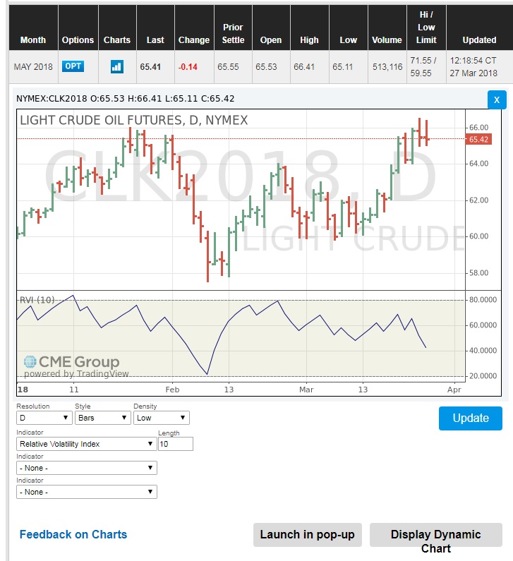
Correlation
Correlation is a measure of the strength of the linear relationship between two quantitative variables. The equation for the correlation coefficient is:
Correlation coefficient takes a value between -1 and 1. As you can see in the following video, a correlation coefficient of 1 indicates a strong positive linear relationship between two variables and a correlation coefficient of -1 shows a strong negative linear relationship. And if two variables are not related or not linearly related, the correlation coefficient can take a value close to zero.
Strength of linear association
The video shows a graph with the explanatory variable on the x-axis and the response variable on the y-axis. There are many points on the graph. The correlation value is shifted from -1 to 1. What the correlation is -1 the points are in a linear, negatively sloped line. As the correlation value changes until the correlation value reached +1 where the points are now in a linear, positively sloped line.
As we learned in a previous lesson, a high correlation between spot and futures market prices makes the hedging efficient. Note that in the case of backwardation, the correlation between spot and futures would be lower.
Example:
The following chart shows the last 10 prices of February 2018 crude oil spot and futures from EIA.
| Date | NYMEX Futures [120]$/bbl | Spot [121]$/bbl |
|---|---|---|
| Feb 14, 2018 | 60.7 | 60.6 |
| Feb 15, 2018 | 61.48 | 61.34 |
| Feb 16, 2018 | 61.89 | 61.68 |
| Feb 20, 2018 | 61.91 | 61.9 |
| Feb 21, 2018 | 61.73 | 61.68 |
| Feb 22, 2018 | 62.72 | 62.77 |
| Feb 23, 2018 | 63.52 | 63.55 |
| Feb 26, 2018 | 63.81 | 63.91 |
| Feb 27, 2018 | 62.94 | 63.01 |
| Feb 28, 2018 | 61.43 | 61.64 |
The following chart displayed the data and, as you can see, they are closely related.
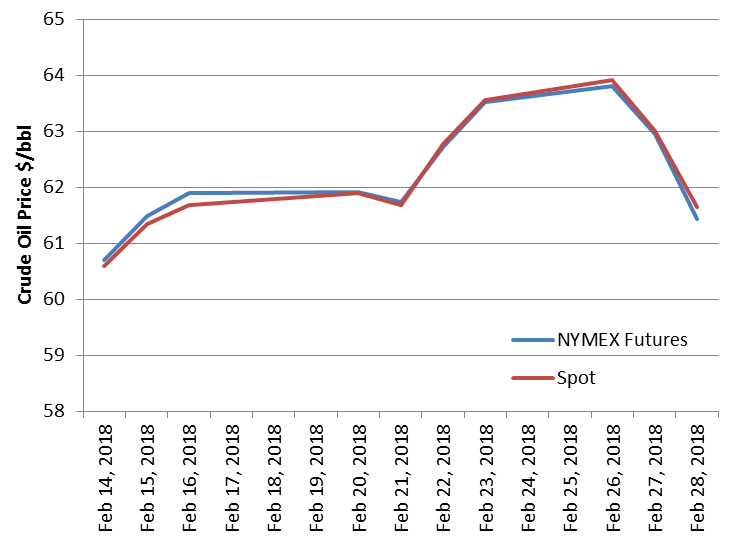
As the following graph shows, we can use the Excel function CORREL() to calculate the correlation between spot and futures for these price data as 0.994, which shows a strong relationship between them.
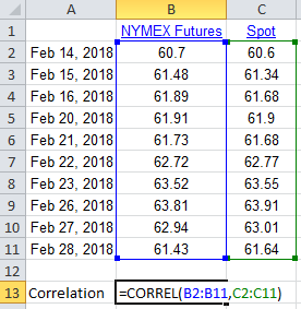
Note that cross hedging is using futures contracts (for commodity A) in order to hedge the price risk for the commodities (commodity B) that don’t have futures contract market. And cross hedging is possible when the futures price of commodity A are highly correlated with spot prices of commodity B.
Note that we can calculate the correlation of the returns in a similar way to what we did to calculate the volatility (calculating the standard deviation for the returns).
Summary and Final Tasks
Key Learning Points: Lesson 8
- Variation of a parameter such as price data is an important factor in risk management.
- A commodity with high price variation is considered a high risk investment.
- Volatility is a term for measuring the dispersion and variation.
- Standard deviation can be used as a measure of volatility.
- The moving standard deviation is the standard deviation calculated for a moving window of data.
- One measure for calculating volatility is the moving (rolling) standard deviation for the changes of price (return).
- Price change can be calculated using an arithmetic method or using the natural log method (return).
- Exponentially weighted volatility uses a decay factor, λ, to apply higher weights to the more recent data.
- Relative Volatility Index is another measure of volatility.
- Correlation is a measure of the strength of the linear relationship between two quantitative variables.
- A strong correlation between spot and futures market prices makes the hedging efficient.
Over the past few weeks, you have been researching various Fundamental Factors that can be used to aid in making trading decisions. In the next two lessons, we will explore quantitative methods and price analysis. The other type of information, used by "day traders," is Technical Analysis. In the next lesson, we will get an elementary overview of Technical Analysis.
Reminder - Complete all of the lesson tasks!
You have reached the end of this lesson. Double-check the list of requirements on the first page of this lesson to make sure you have completed all of the activities listed there before beginning the next lesson.
Lesson 9 - Technical Analysis
Lesson 9 Introduction
Overview
Thus far, we have addressed the fundamental factors that influence energy prices. We also established that there are two main groups that trade in the financial energy commodities markets, commercial and non-commercial. The latter group represents the “pure” traders or “speculators." These participants are only interested in price movement. The type of commodity does not matter to them. In order to make trading decisions, they use technical analysis as opposed to fundamental analysis.
Technical analysis involves the use of charts to track price movement, establish the current market trend, and determine the probability of prices moving in one direction or another. Simply put, technical or “day” traders are interested in market activity as illustrated by the resulting prices.
Since the prices that occur in the market are the result of human decision-making, technical analysis really examines the behavior of market participants. As such, patterns emerge that have a high probability of recurring. It is precisely these events that technical traders are looking for. But, make no mistake; fundamental events cause traders to react emotionally, the results of which are also reflected in the price action.
In technical analysis, traders must first establish what the current price trend is, up or down. Then, they must determine the probability of the trend lasting or changing direction. It is this information that guides their buy/sell decisions.
Learning Outcomes
At the successful completion of this lesson, students should be able to:
- distinguish the difference between technical and fundamental market analysis;
- identify different types of technical charts and their uses;
- recognize trend lines and market signals;
- analyze “momentum” indicators.
What is due for this lesson?
This lesson will take us one week to complete. The following items will be due Sunday at 11:59 p.m. Eastern Time.
- Lesson 9 Quiz
- Lesson 9 activities as assigned in Canvas
Questions?
If you have any questions, please post them to our General Course Questions discussion forum (not email), located under Modules in Canvas. The TA and I will check that discussion forum daily to respond. While you are there, feel free to post your own responses if you, too, are able to help out a classmate.
Reading Assignment: Lesson 9
Reading Assignment:
Seng - Chapter 10
Errera & Brown - Chapter 8
This text is available to registered students [112] via the Penn State Library.
Key Points of Emphasis
- Technical analysis relies on the principles of probability and statistics.
- The (3) most popular technical charts are Line or "close only," Bar, and Candlestick.
- Line charts record only the daily closing price and are best used for long-term trending.
- Bar charts indicate the daily Open, High, Low, and Closing prices for the trading day.
- Candlestick charts also show the OHLC but do so in a fashion as to illustrate the market direction, up or down, for that day's trading.
- Identifying the current trend is the first step.
- Determining if the trend is going to change is the next step. This can be ascertained if the preponderance of the evidence indicates it will. Buy/sell decisions will then be made.
- Trend lines are used to indicate the trends.
- Various price patterns exist for traders to identify.
- Volume is a good indicator of market activity and can reinforce the day's price movement.
- Resistance is the price level at which sellers enter the market again. It establishes a "ceiling" price in the current market.
- Support is the price level at which buyers enter the market again. It establishes a "floor" price in the current market.
- Moving averages are good studies to utilize if you believe in the statistical premise of "reversion to the mean."
Charting Methods
There are several types of charting methods, but three of them are the most popular.
Bar Chart
In a bar chart, a vertical line is shown for each time increment selected. In the chart below, a “daily” chart is used to show the May NYMEX contract for natural gas. Each bar shows the price results for that day’s trading. The mark to the left of the bar represents the first trade of the day, or the “Open.” This is the price of the first trade that occurs right after the bell rings to start trading. The vertical line itself represents the full range of prices for the day, that is, the High and Low prices. And the mark to the right of the bar represents the final closing, or “Settlement” price for the day. This is often referred to as the "OHLC" chart (Open/High/Low/Close). Note that if the Open price is lower than the Close, the bar is green. If the Open price of the day is higher than the Close price, the bar is red. It shows the direction of the market movement; do prices tend to go up or down?
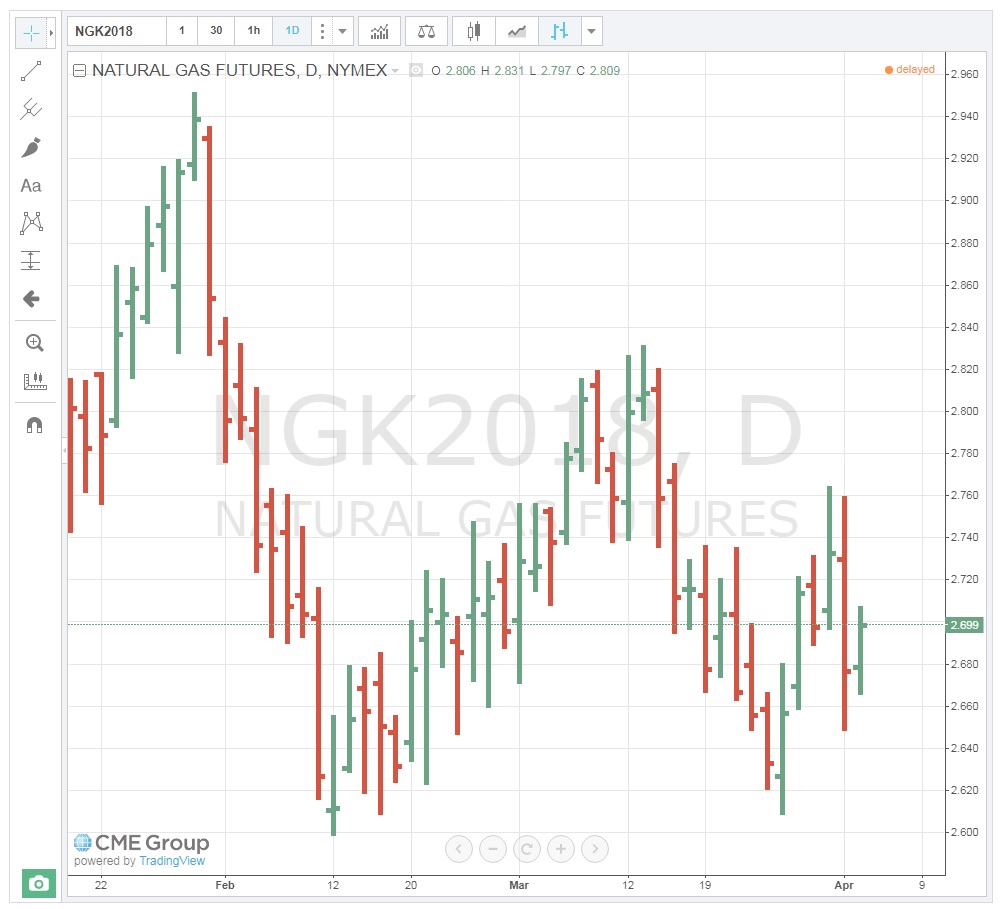
Style of Charts
You can change the style of the chart and type of information that you want to be displayed by clicking on the Bar Style toolbar  and selecting from the list of chart options which include things like bars, candles, line, area, and point & figure. The image below is an example of a “Line” or “Close Only” chart showing the same May natural gas contract. You will notice that it only shows the daily market closing (settlement) price. It provides much less information than the Bar chart and is mainly used for longer-term trend analysis.
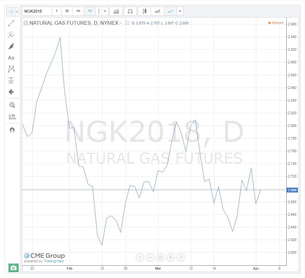
Candlestick Charts
Candlestick charts were developed by the Japanese centuries ago. They provide information similar to the Bar chart, but also indicate “up and down” days. That is, they clearly show the direction the market took on a daily basis. The top end of the “candle” still represents the "High" for the day, and the lower end represents the “Low,” but the “body” indicates the Open and Closing prices in relation to one another. For example, if the Open is higher than the Close, the Open price is at the top of the “body” of the candle and represents a day where prices fell (red candle). Conversely, if the Close is found on the top of the “body,” it represents an “up” day, and on the chart below, appears with a green “body.” As you can now see, the up-and-down days are easily visible on the Candlestick chart. By counting these, we can determine the current trend. For traders, the question is, when will it reverse course?
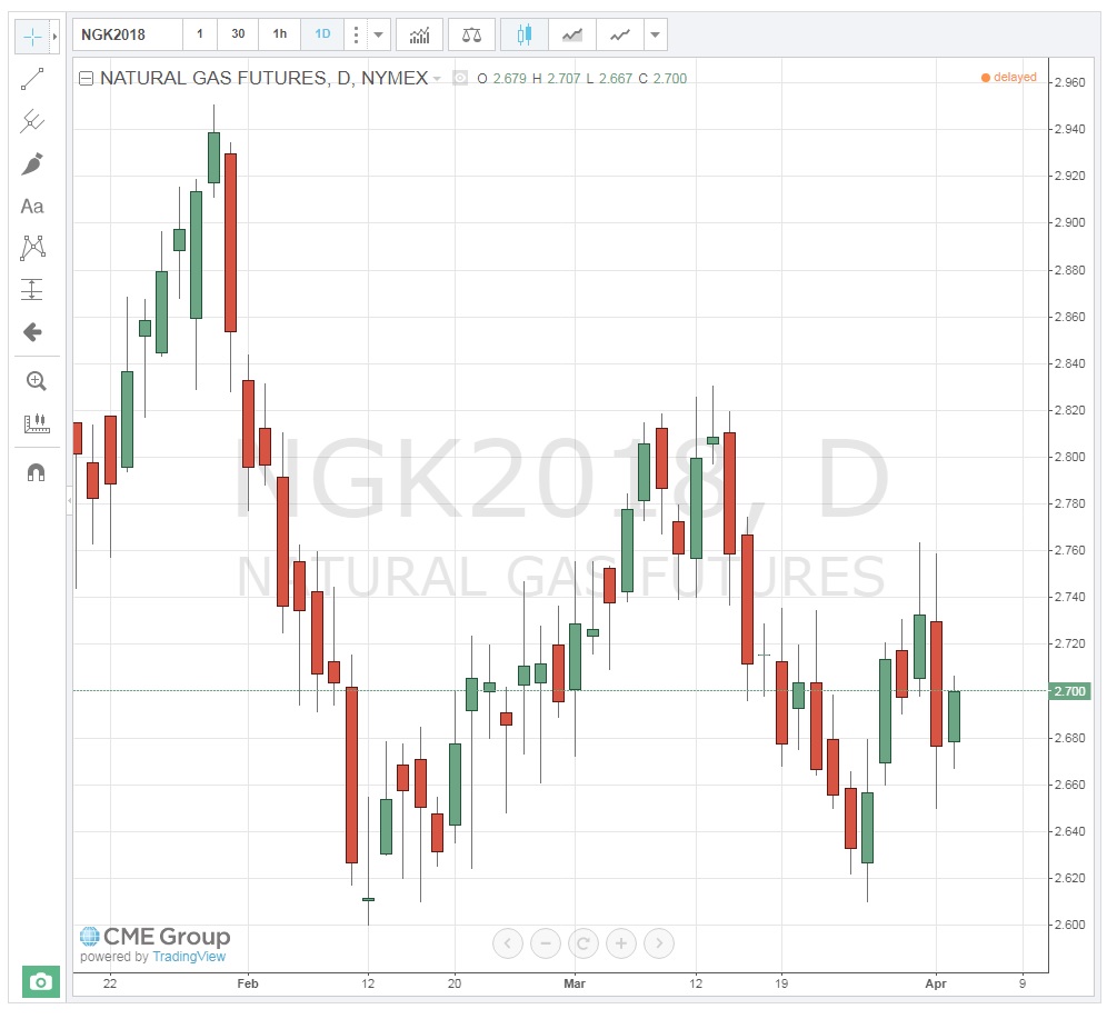
Trendlines
Trend lines can be used to identify both long- and, short-term price trends. They are also used to indicate support and resistance prices and channels (covered later). A trend line only has significance if it touches at least two price points. The chart below shows an obvious long-term downtrend going back one year.

This next chart illustrates two short-term trendlines, one up and one down.
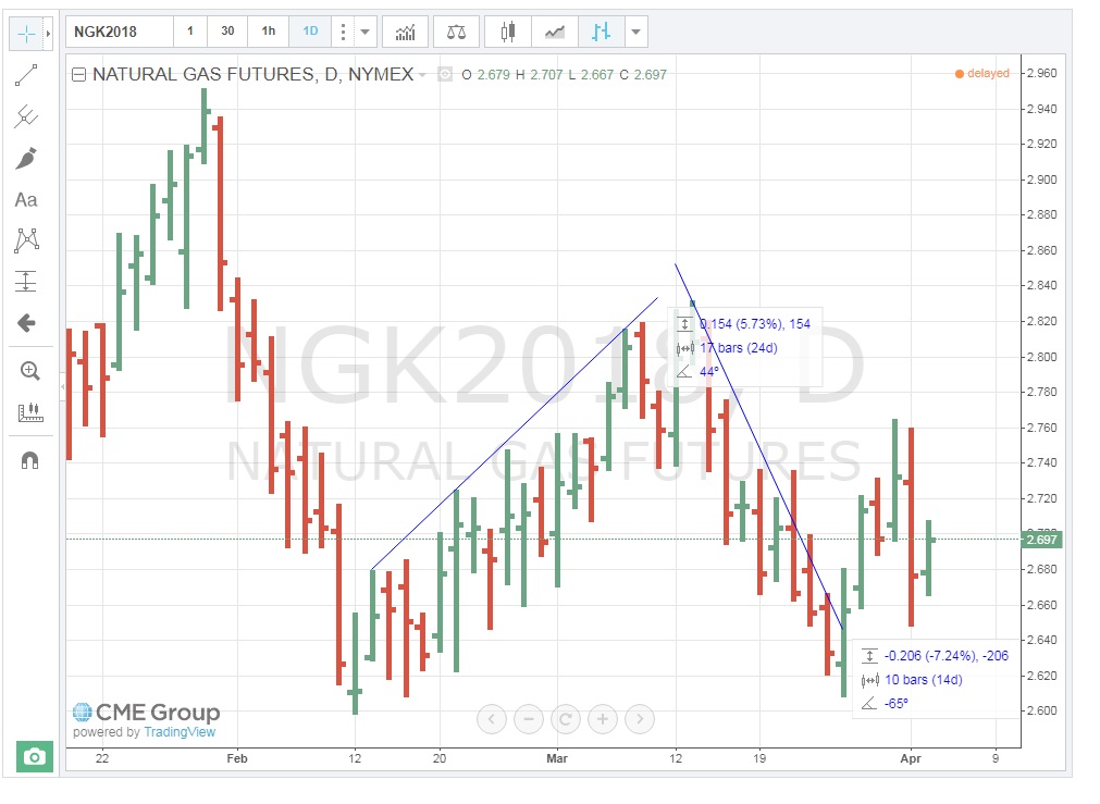
When one trendline connects two or more price points and another trendline connects two or more price points in parallel fashion, they form a “channel,” as shown below. Channels have significance in that traders look for prices to move above or below the confines of the channel. This is referred to as a “breakout,” and depending on the number of days that form the channel, this can occur with good momentum, resulting in a large price move in that direction.
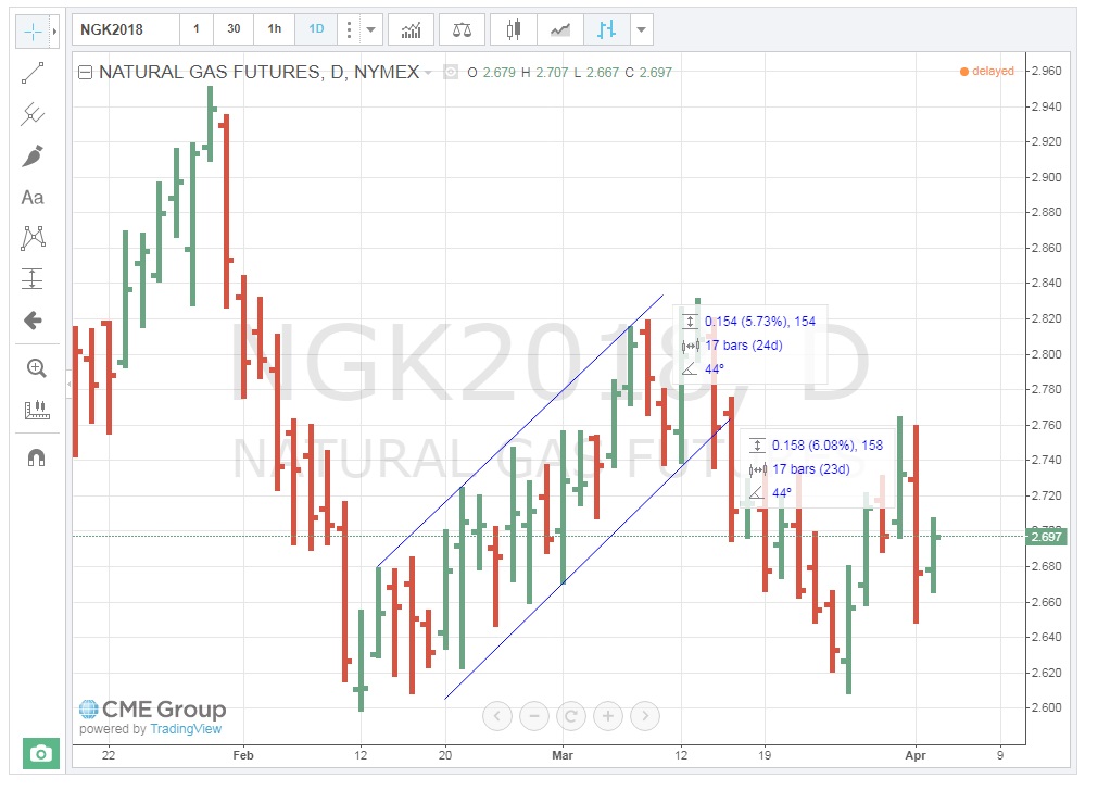
Trend Indicators
Volume
One of the simplest clues to the strength of price movement is that of the volume of contracts traded. If a price shows a large range or change in direction on a particular day, looking at the volume of contracts traded indicates how well-supported that move was by the market participants. A $0.10 movement up or down in natural gas is not very significant if a low volume of contracts is traded. On the other hand, when large volumes trade, that definitely reinforces the price action for the day. It’s as if those trading have agreed on the price outcome. The chart below is a Daily Bar Chart with volume for natural gas. Notice that on April 1st, prices traded in a $0.1 range and a very large amount of contracts exchanged hands, solidifying the move. Also, on March 27th, the second-highest volume for the contract traded. Both of these volumes add legitimacy to the price action for those days.
You can add the volume traded to the chart by clicking on “Indicators, …”  on the toolbar and choosing the "Volume" from the resulting list.
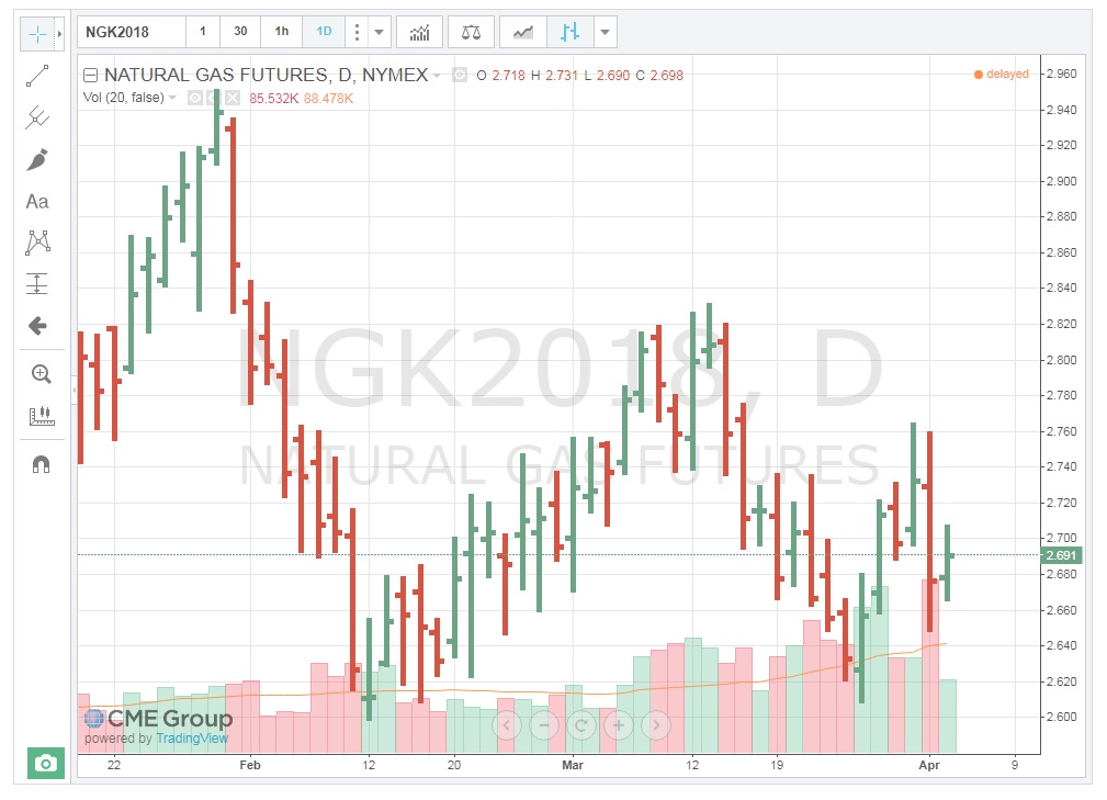
Moving Averages (MA)
For those of you who have had statistics, you should be familiar with the term “reversion to the mean.” For those of you who have not, the concept hinges on the idea that all prices will eventually return to their average, despite dramatic movements up or down. I have found this to be especially true for energy commodities, at least in the short-term. Therefore, tracking commodity moving average prices can be a good signal for a change in the direction of a trend. The chart below shows that the Moving Average (MA) for May 2018, Natural Gas. If prices go up, there is a good probability that they will eventually fall towards the MA. It may be a gradual decline which also means the average will change, but as long as the MA is lower, prices will gravitate towards it. The exact opposite occurs when prices fall below the MA.
Note that the timeframe for the MA is set to the particular trader’s needs. I have set the MA at 5 days, as that represents a full week of trading (regular session, pit trading only occurs on weekdays). See how the prices, while moving above and below the MA, ultimately return to it. This is a key sign for making buy/sell decisions.
You can add the Moving Averages traded to the chart by clicking on “Indicators, …” on the toolbar and choosing the "Moving Average" from the resulting list.
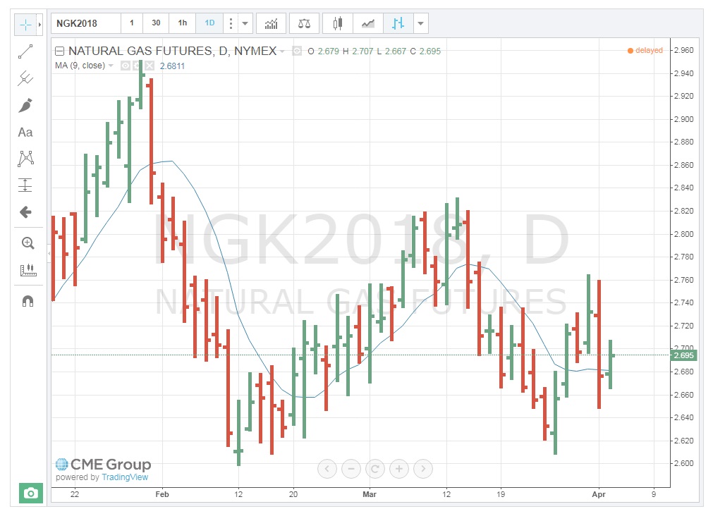
Relative Strength Index
Relative Strength Index (RSI) is a momentum oscillator that measures the speed and change of price movements. RSI oscillates between zero and 100. Traditionally, RSI is considered overbought when above 70 and oversold when below 30. RSI can also be used to identify the general trend. (Technical Indicators and Overlays - ChartSchool [122]) Understanding the exact RSI calculation is not necessary to understand how to use this indicator. The next chart is a Daily Bar Chart with Volume, MA, and now, the RSI study. Note that the current RSI is over "70" which is considered “overbought". This could, therefore, be a signal to "sell."
You can add the Relative Strength Index traded to the chart by clicking on “Indicators, …” icon on the toolbar and choosing the "Relative Strength Index" from the list.
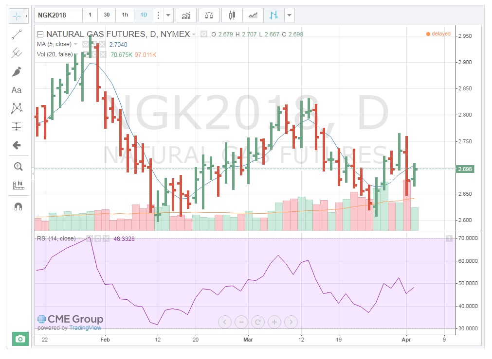
Price Signals
As with trend analysis and market indicators, there are several types of price signals. We will deal with a few of the ones that are more common and easy to use.
Support & Resistance
As prices move up and down, traders make decisions as to when to continue to buy in an uptrend and when to sell in a downtrend; that is, they try to determine when the current trend will exhaust itself and change direction. One way to do this is to look at the “support” and “resistance” price levels. Support represents a price level at which buyers will step back into the market after a period of selling. This interest establishes a “floor” price. Traders find value at this level and start to buy-up the contracts again. In some cases, traders who have been selling contracts during the downtrend may be buying them back to take some profits. Resistance is the price level at which the market is no longer interested in buying contracts. The price is deemed to be too high and sellers re-enter the market, thus establishing a "ceiling" price.
So, how do we establish these pricing points? As the chart below (shifted to the right) shows, when we draw upper and lower trend lines, the lines continue through price points on the right, vertical axis. Where the upper trend line crosses the right axis is the resistance point, while the price where the lower trend line crosses the right axis is the support point. Theoretically, then, these represent both the maximum the market is willing to pay as well as the minimum at which it is willing to sell.
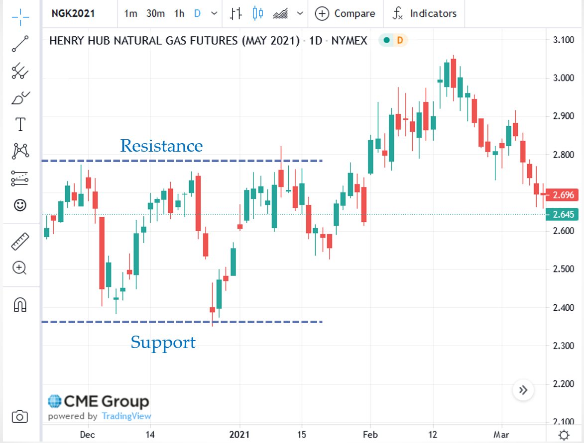
This chart indicates that resistance and support. Traders will now look to see if prices can trade above, or below, these levels. If they do, there will be a flurry of activity in the direction of the move.
Tops & Bottoms
Since we are on the subject of support and resistance, we can discuss price signals related to those concepts. As we have said, traders are interested solely in price movement. And support and resistance levels represent buying and selling interest. So, what happens when the buyers or sellers step in to halt the moves higher or lower? They are testing the points of support and resistance. If the sellers can’t break through support, it is a result of buyers stepping in. As mentioned above, that sets a “floor” or “bottom” price on that day. Likewise, if buyers test the resistance price and sellers step in to prevent a breach of that level, a “ceiling” or “top” is established.
While a one-day occurrence of these events is not a very strong indicator of a change in direction, the more a “bottom” or “top” is tested and holds, the more significant that price level becomes. Think about it this way. Let’s say natural gas Traders are trying to sell May contracts and push the price down to the $2.37 Support level on the chart above. Buyers step in at that price and the sell-off fails. The next day, Sellers again attempt to push prices down to $2.37, and again, the move fails.
Let's assume the market now begins to see $2.37 as a stronger Support price. We refer to this as a “double-bottom.” While this is still a good indicator of price levels, a third day, or “triple-bottom” is a strong indicator that prices could rally higher. Traders have no choice but to recognize the buying interest at $2.37 and thus will buy contracts until the Resistance, or “top” is tested. The same holds true for resistance levels, but in reverse. The more “tops” are established, the stronger the level at which sellers will step in and sell contracts.
"Head-and-Shoulders" Reversal Patterns
Head and shoulder reversal patterns are identifiable, price patterns that signal a change in direction and can be used for long-term or short-term trend analysis. This consists of three trading days where the middle day’s High, or Low, is higher or lower than that of the other two days. The first day then represents the “left shoulder,” the second day is the “head,” and the third day is the “right shoulder.” Using the chart below without all the trend lines, we can see that on June 14th, the High for the day was higher than the 3rd. We are now looking for the completion of the pattern, the right shoulder. And on June 22nd, the High for the day was lower than the head. Now you can see the pattern whereby the 3rd is the “right shoulder,” the 14th is the “head,” and the 22nd is the “right shoulder.” The right shoulder “leans” in the direction of the price change. In this case, prices reversed from an uptrend to a downtrend. There are also “reverse” head-and-shoulders patterns. These occur in an upside-down fashion and signal a move from a downtrend to an uptrend.
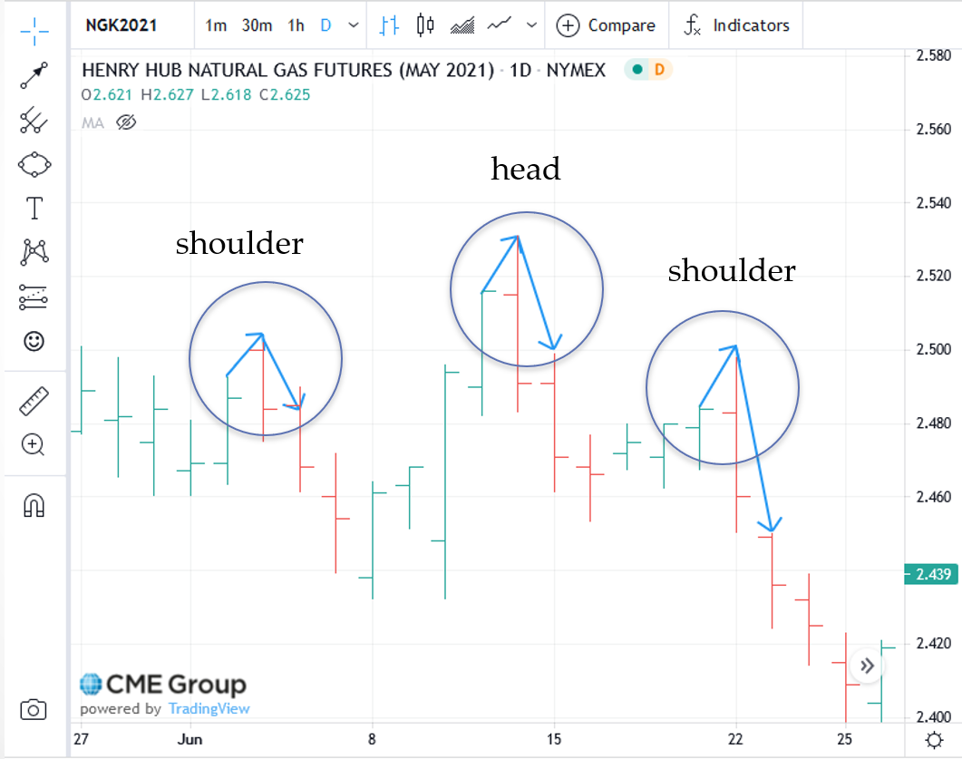
"Consolidation” Patterns
When upper and lower trend lines are drawn and are parallel to one another and perpendicular to the Y-axis, they form a rectangular shape. The upper trendline does represent resistance, with the lower trend line indicating support. In this pattern, prices will move up-and-down within the rectangle. This “consolidation” is indicative of market indecision. Traders are not really sure what direction prices should take. It is a battle between buyers and sellers. The key here is the number of days this pattern continues to exist. The longer traders battle, the more momentum builds-up for when prices break-out of this range. Think of it as a spring that winds tighter and tighter for each day prices stay within the consolidation range. That means a very large price movement will occur in the direction of the breakout. A good illustration of this is the May 2021 crude oil contract, shown below. Starting in January, the contract bounded by a Low of about $52 for twenty-four straight days. The High was about $54 with the exception of attempted "break-outs". On February 2nd, prices broke-out to the upside with good momentum.
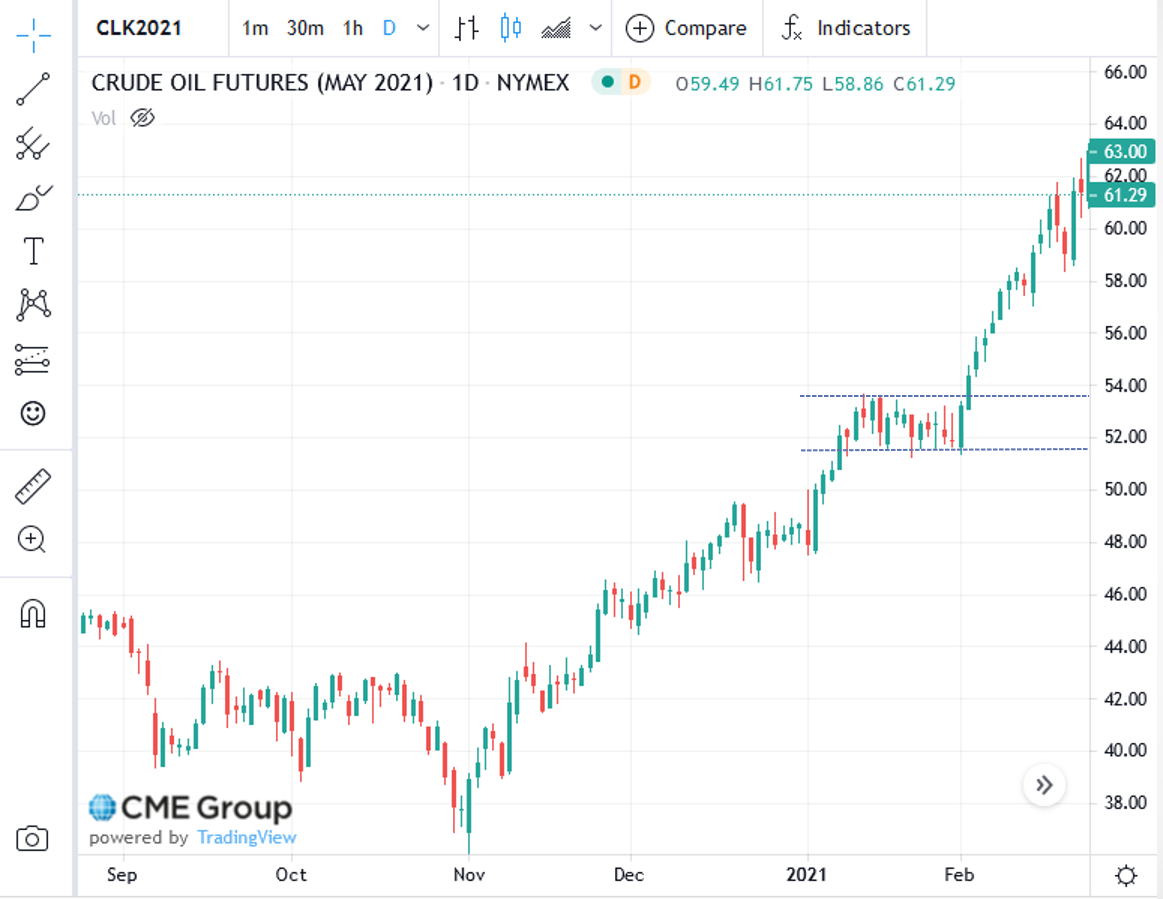
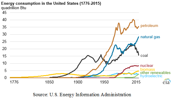
These are but a few of the methods in Technical Analysis used to try to determine when a greater probability exists of prices moving in one direction vs. another. Once determined, traders enter or exit the market at those price levels.
Summary and Final Tasks
In addition to my explanations, the definitions of terminology used in Technical Analysis can be found at:
Technical Indicators and Overlays - ChartSchool [122]
Key Learning Points: Lesson 9
- Technical Analysis is mainly used by “day” traders, or speculators, to determine the greater probability of one thing happening over another (price direction).
- By plotting prices, technical charts actually record the behavior of the market participants. Technical analysts look for these patterns to repeat themselves.
- There are (3) main types of technical charts used:
- daily bar chart, which shows the “Open/High/Low/Close” prices;
- “close only” or line chart, which shows the settlement price for each time segment;
- candlestick chart, which shows the same information as the daily bar chart, but also indicates “up and down” days.
- Trend lines are used to identify current and past trends, but must touch-on at least two pricing points to have significance.
- Examples of simple trend indicators are:
- volume – this illustrates the amount of activity behind the price movement, which either reinforces it or fails to support it;
- moving averages – traders look to the statistical “regression to the mean” as a predictor of price direction;
- relative strength index – a momentum indicator that identifies both the speed and change in price with a resultant “overbought,” “oversold,” or “neutral” market condition.
- Examples of price signals are:
- support – the price level at which buyers will step in, establishing a “floor”;
- resistance – the price level at which sellers will step-in, establishing a “ceiling”;
- “tops and bottoms” – these are recurring Highs or Lows that “hold,” thus establishing strong support or resistance. Double or triple tops and/or bottoms are very strong indicators of a possible change in price direction;
- “head-and-shoulders” reversal pattern – a 3-day price pattern whereby the middle day’s High or Low is higher or lower than the other two, thus forming a “left shoulder,” “head,” “right shoulder” configuration. The right shoulder “leans” in the direction of the price change;
- “consolidation” – this represents several days of trading stuck within a certain High/Low range. It indicates price indecision by the market and a “battle” between buyers and sellers. The more days within the pattern, the greater the velocity of any “break-out” of the pattern.
In the next lesson, we will explore other, more advanced, financial derivatives that can also be used for hedging. Among these are "swaps", "spreads", and "options". They are mostly traded in the "over-the-counter" markets, that is, non-exchange traded. "OTC" encompasses electronic trading platforms as well as "voice" brokers where transactions occur over the phone.
Reminder - Complete all of the lesson tasks!
You have reached the end of this lesson. Double-check the list of requirements on the first page of this lesson to make sure you have completed all of the activities listed there before beginning the next lesson.
Lesson 10 - Advanced Financial Derivatives - Swaps, Spreads, and Options
Lesson 10 Introduction
Overview
In Lesson 7, we focused on “futures” markets and how simple hedges can be accomplished using exchange-traded contracts. Those provide the "building blocks" for the more advanced hedging tools. Here, we will address the “over-the-counter,” non-exchange traded markets, or “forward” contracts. Keep in mind that NYMEX Exchange contracts are referred to as “futures.” We will also cover financial “spreads” whereby traders take advantage of price differences based on location, time, or inter-commodity relationships. Finally, we will deal with financial options, which are a simpler and less costly form of hedging vs. the financial derivative contracts themselves.
Key Learning Points – Energy Risk Hedging Using Swaps, Spreads, and Options
- Exchange-traded energy contracts are known as “futures,” whereas non-exchange traded contracts are known as “forwards."
- These are traded on electronic trading platforms or over the phone with licensed brokers.
- “Swaps” are exchanges of payments between two parties. They are strictly financial. No physical exchange of the commodity takes place.
- One party to the transaction agrees to pay a current market price (“fixed”) while the other agrees to pay a price in the future (“floating”) which is the "settlement" price for this arrangement.
- They are a simpler and less expensive way to hedge price risk as the price difference is what matters and not the price itself.
- One very important swap is natural gas “basis swap,” which is a market-determined value that represents the difference between the NYMEX Henry Hub contract delivery point for natural gas and other physical (cash) natural gas trading points in North America.
- Spreads are merely price differences between commodities that are interrelated somehow, have differing locations, or represent different months of the same commodity.
- They are traded for hedge purposes (reduce price risk) or outright trading (speculate on price spread movement).
- Energy options are yet another, simpler way to hedge price risk. They are less expensive than the outright purchase or sale of the underlying contracts. We will cover the types of energy options and their uses:
- call options
- put options
- hedging with options
Learning Outcomes
At the successful completion of this lesson, students should be able to:
- explain the following financial derivatives and their uses:
- swaps,
- spreads,
- options;
- comprehend the importance of the natural gas basis swap and its application in hedging locational price risk;
- apply advanced financial derivatives to energy commodity hedging;
- list the components of an options contract;
- outline the inputs to the Black-Scholes model for options valuation
What is due for this lesson?
This lesson will take us one week to complete. The following items will be due Sunday at 11:59 p.m. Eastern Time.
- Lesson 10 Quiz
- Lesson 10 activities as assigned in Canvas
Questions?
If you have any questions, please post them to our General Course Questions discussion forum (not email), located under Modules in Canvas. The TA and I will check that discussion forum daily to respond. While you are there, feel free to post your own responses if you, too, are able to help out a classmate.
Reading Assignment: Lesson 10
Reading Assignment:
Seng - Chapter 7, 8, and 9
Errera & Brown - Chapters 4 & 6
This text is available to registered students [112]via the Penn State Library. [73]
Key Points of Emphasis
- Non-exchanged traded financial derivatives are known as "over-the-counter" (OTC).
- Swaps and spreads trade OTC while options are exchanged and OTC traded.
- Swaps are exchanges of payments between two buyers are financially settled.
- Swaps are normally "fixed-for-floating" whereby one price is the current market price ("fixed") and the other price is the future settlement price ("floating").
- Spreads are trades which occur between commodity locations and times, as well as intra-market and inter-market.
- Options give the holder of the option the right but not the obligation to buy or sell a commodity at a particular price for a specific date and location in the future.
- Options are price risk insurance, and a premium is paid for options contracts.
- Premiums paid are substantially less than the outright commodity contracts.
- Option premiums are determined using mathematical models. The most well-known is the Black-Sholes.
- "Put" options give the buyer a "floor" price, whereas "call" options establish a "ceiling" price for the buyer.
- Options buyers are only exposed to the cost of the premiums.
- The seller (writer) of an option assumes all the risk.
Financial Energy Swaps
Swaps represent exchanges of payments between two parties. They are financially settled, and no physical commodity is delivered or received by either party. They represent a substitute for the futures contracts but rely on NYMEX pricing to establish the financial arrangement for the swap contract. Similar to a NYMEX contract, the elements of a swap contract include the commodity, location, date, and price.
We use the phrase “fixed-for-floating” swap to signify the prices agreed to by both parties in the contract. The “fixed” price is always the current market price. It is the price known at the time the deal is struck. The exchange of payments will occur when the NYMEX settlement price is known. We refer to this settlement price as the “floating” one, since it is not known until the contract’s last trading day and “floats” with each day’s trading until then. The difference between the two represents the amount of payment due to one party or the other.
For example, as of this writing, the December 2019 NYMEX crude oil contract is trading $62.69. If I bought a swap, I would be setting my contract price at $62.69. On November 20th, 2019, this contract will settle, and the difference between my $62.69 and the NYMEX Final Settlement price that day, will be the amount exchanged between me and my counterparty. If the contract settles at $63.19, since I bought the swap, I would be selling it back at that price for a profit of $0.50 per contract and, my counterparty would pay me $0.50 per contract (1,000 Bbl), or $500. On the other hand, if the contract settled at $62.19, I would be selling the contracts back at a loss of ($0.50) and I would pay my counterparty $0.50 per contract, or $500. The calculations are the same as those shown in Lesson 7's hedging spreadsheet.
As we learned in previous lessons, Futures contracts are standard contracts. However, swaps can be customized. This is another advantage of swaps that make them popular. The advantage of using swaps for hedging is that you can achieve the same price protection without actually having to buy or sell NYMEX contracts. And you can work with brokers either by phone ("Voice" Brokers) or through an electronic trading platform such as "The Intercontinental Exchange (ICE)".
In a previous lesson and in the textbook, we discussed the fact that physical entities wishing to hedge must take a position in the financial market which is the opposite of their physical position. For instance, a crude oil producer is "long" the commodity. Therefore, in order to execute a proper hedge, they must go "short" in the financial derivative they choose. In Lesson 7, I presented how the physical and financial prices interact in a hedge. The same applies to swaps as to the NYMEX contracts themselves.
Key Learning Points for the Mini-Lecture: Financial Energy Swaps
- “Swaps” are exchanges of payments between two parties. They are strictly financial. No physical exchange of the commodity takes place.
- One party to the transaction agrees to pay a current market price (“fixed”) while the other agrees to pay a price in the future (“floating”).
- They are a simpler and less expensive way to hedge price risk.
- One very important swap is a “basis swap” which is a market-determined value that represents the difference between the NYMEX Henry Hub and other natural gas trading points in North America.
- For basis swaps, the "fixed" price or, "known" is the current market price which can be obtained through electronic platforms such as NYMEX Clearport or ICE. In addition, some brokers will give quotes over the phone. The "floating" price becomes known when the NYMEX contract for the particular month settles and the monthly index ("postings" we addressed in Lesson 5) for the cash location is published. This is known as the "actual" or "settlement" basis and represents the other value in settling the swap.
The following mini-lecture is a summary of the points presented above (3:37 minutes).
In this lesson, we're going to talk about some of the more advanced financial derivatives. Now, you'll find some pretty extensive notes in the actual lesson content page, so I'm going to do a summary here with these slides. And the first financial derivative that we're going to talk about is a swap.
Now, a swap is an exchange of payments between two parties. It can be a form of hedging, it can also be used for outright trading, so speculative traders can use swaps to try and make some revenue. These are generally known as over-the-counter. That is, they're not traded on an official exchange, such as NYMEX, but you do find them on electronic platforms, such as NYMEX's clear port or the Intercontinental Exchange. And then, also, swaps can be had by dealing with the so-called Voice Brokers-- literally a broker that you call up and arrange for a swap transaction. Now, these are strictly financial. In most cases, there is no physical commodity involved. You're strictly swapping out price.
Now, there are two pieces in a swap agreement. One is a fixed price and the other is a floating price. So, we refer to swaps as fixed for floating. One party will pay a fixed price at the time that the swap is actually entered into. And the other pays the floating price, and that's the price that is not known at the time. You have to wait till settlement of the respective underlying contract.
Now, we talk about the NYMEX look-alike because it's the most commonly used swap. It's a Henry Hub financial swap, and one party buys or sells at the current market, which would be the fixed or known price, in other words, whatever the NYMEX is currently trading at. And then the counterparty buys or sells, so the opposite party is going to take the opposite position. They'll buy or sell based on the NYMEX settlement. Now, this is your floating price, and it's unknown at the time of the swap transaction. So, in other words, the price floats as we know every day as NYMEX changes.
So, you set a price on the day that you enter into the swap for the specific month and the commodity that you are interested in. And then, in essence, the two counterparties, you and your counterparty, are going to wait until the NYMEX contract settles. And then, you're going to go ahead and true up, see who owes who money. And again, it's financially settled every month.
And then, we've also addressed the basis swaps. Again, there's more detail and specific examples in the lesson content. But really, in the case of a basis swap, we're looking at the current market value.
Now, the current market value you can find on NYMEX's clear port system. Or, if you have access to the Intercontinental Exchange, you will see natural gas basis swaps quotes for the various cash locations that we have reviewed in the publications, such as Platt's. And then, we have to come up with the second part of this, in other words, the floating price. We can fix the price based on the values on those electronic platforms I mentioned. But then, to settle with our counterparty, we have to wait until the settlement of the basis. Now, we know when a NYMEX final settlement occurs, and so we'll have that piece of the basis swaps settlement, but then we're waiting for the cash prices to come out. So, in other words, Platt's has their monthly price guide, or as I noted, it's more commonly known as the Inside FERC postings. So, those are the first-of-month cash prices for the respective location. And when you take the NYMEX settlement, and you find that cash location, that difference becomes what we call actual basis. It is the settlement price for the basis swap for that particular location.
Financial Energy Spreads
“Spread” trading can be used for hedging purposes or purely for trading (“arbitrage”). Spread trading involves taking a long position in one futures contract and simultaneously taking a short position in another, related futures contract. Thus, spread consists of two equal and opposite futures positions. In spread trading, futures or forwards can be used to achieve the desired results. A buy/sell is offset by a corresponding sell/buy. Spread trading involves using price differences in futures or forwards based upon inter-market (time differences, locational differences) and inter-market commodity relationships.
Examples of the types of spreads are:
- Inter-market (inter-commodity) Spread – Buy/sell differing but related commodities
- “Crack” Spread
Buy crude oil/sell heating oil or gasoline (HO/RBOB is “cracked” from CL). - “Frack” Spread
Buy natural gas/sell propane (midstream natural gas companies process natural gas into propane and other NGLs). - “Spark” Spread
Buy natural gas/sell electricity (electric generators can use natural gas to produce power).
- “Crack” Spread
- Intra-market (intra-commodity) Spread – Buy/sell same commodities
- Time Spread (often called a “storage” spread)
Buy a natural gas contract in May/sell it in January.
Buy a heating oil contract in April/sell it in December. - Locational Spread
Buy NYMEX crude (WTI) contract/sell Brent (North Sea) crude contract.
Buy NYMEX Henry Hub natural gas/sell a different cash market Hub ("Basis" value).
In addition to traders who are merely interested in price movement to make money, commercial entities can use spreads to hedge their price risk. For example, as mentioned above, a crude oil refiner can buy crude contracts (hedge price of feedstock) and sell heating oil and unleaded gasoline contracts (refined output) to establish a profit margin or “crack” spread. This hedge is illustrated in the spreadsheet, "EBF-301 Lesson 10 refinery hedge.xls" found in Canvas Lesson 10: Advanced Financial Derivatives - Swaps, Spreads, and Options Module.
Key Learning Points for the Mini-Lecture: Financial Energy Spreads
- Spreads are merely price differences between commodities that are interrelated somehow, have differing locations, or representing different months of the same commodity.
- They are traded together for hedge purposes (reduce price risk) or outright trading (speculate on price spread movement).
The following mini-lecture summarizes the points presented above (6:10 minutes).
Moving on to the next part of our discussion of advanced financial derivatives, we're talking about spreads. Again, I've got some extensive notes and some examples in the lesson content, but we'll review these concepts here in these slides.
OK, Spread trading itself-- here we're talking about trading-- it's a technique that takes advantage of the relative price movement between futures contracts. Arbitrage, that's a simultaneous purchase and sale of similar or identical commodities in two different markets in hopes of gaining a profit from the price differential. Now again, with spread, we're not dealing so much with price as we are dealing with the price differences. Margin requirements are considerably lower than the requirements on single futures contracts, because again, the exposure is the spread difference-- the difference between the price is not one singular price. So that also makes them less risky than outright futures positions. You're exposed to this movement in the spread, either the spread widens or the spread gets tighter, as opposed to the price of the futures contracts themselves.
Here are some simple rules. This is for trading spreads for speculative purposes. Rule 1 is, if you think spreads are going to narrow, you buy low, and you sell high currently. So, you buy the lower price, and you sell the higher price to set a spread. And then, when the prices do, in fact, narrow based on your expectations, you'll be able to go ahead and liquidate that spread at some profit. Otherwise, if the spreads are expected to widen, you expect the price difference to get greater, you will buy the high contract now and sell the lower of the two.
Different types of spreads-- one is the Inter-market. Now, this is the simultaneous purchase and sale of different, but related, commodities that have a reasonably stable relationship to each other. So, inter-market, keep in mind, inter-market means different commodities, not the same commodity. So, we have some different types of spreads and these are the commonly used terms for these spreads.
We have what's known as a Crack Spread. OK, this would be crude oil versus unleaded or heating oil. Now, if you think back to the lesson on crude refining, you have a process by which you are actually cracking the hydrocarbon molecules and then reforming them into these other products, so that's why you get this name here. Crude being the feedstock, and the refined products being unleaded and heating oil. And all three of these trade on the New York Mercantile Exchange. Therefore, these can be used to hedge the spread that refiners are exposed to.
A Spark Spread, it's natural gas versus electricity. Again, this would pertain strictly to natural gas fired power plants. Heating oil versus gas oil-- again, this one can be broken down into another, so we can use this spread. NYMEX versus ICE. Now, this is on crude oil spreads. Here, we have a situation where we're actually using inter-markets. The markets are the different trading platforms. So, savvy traders can sit there and look at NYMEX prices and Intercontinental Exchange Prices for crude oil, and they can take advantage by buying one and selling another, or selling one and buying another electronically.
And then we have a Frac Spread, and this is not to be confused with fracking, which is a completion method for oil and gas wells. What we're talking about here is, again, if you think back to the lecture on processing, the processing plants take natural gas and convert it to natural gas liquids or the so-called fractions using a fractionation tower. And so, that's where we break down and get the ethane, propane, butane, isobutane, natural gasoline, and condensate. So, since natural gas is the feedstock for a processing plant, and the natural gas liquids are the output from that plant, we can put on a frac spread to hedge those differences.
The other type of spread is Intra-market, and this is also known as an intra-commodity spread. The idea here is we are using the same commodity, but we are trading things like time or location. So, a time spread is the simultaneous purchase and sale of futures contracts on the same commodity for different delivery months. So, for example, we could buy August 2015 natural gas contracts and sell the January 2016 natural gas contracts. This would be a storage spread, because the idea would be we would buy the August contracts, put that gas in the ground in August, and then turn around and sell the January contracts, and take the gas out then. So, that difference in price between August and January represents our storage spread.
Then we also have Locational Spreads. This would be the simultaneous purchase and sale of futures contracts for different locations. So, for instance, in terms of crude, we could use the WTI versus the Brent crude pricing. And for natural gas, we could use Henry Hub versus, say for instance, New York City. And here's an example of an intra-market spread for natural gas. Again, as I've mentioned right here, in this example, we're going to talk about August 2015 versus January 2016 at these respective prices.
So, if you think spread's are going to narrow, in other words, we start up $2.90 versus $3.25, so we have a $0.35 spread, if you think that that spread is going to become less, you're going to buy the low, which is the $2.90 and sell the $3.25, which is the high. And then, if you think spread's is going to widen, that is that the price difference between these two months is going to end up being greater than for $0.35, you're going to sell the lower priced, $2.90, and you'll buy back the $3.25. Now, again, keep in mind this is for speculative trading, trading for pure profit. This is not a hedging type of plan or scenario.
If one wishes to enter into a contract for underground storage capacity, this transaction can be hedged as well using the time spread.
Example of Time Spread:
Let’s look at an example. The April 2020 NYMEX natural gas contract is trading $2.65 at the time of this writing. We can buy these contracts and that will represent the supply that we would inject into storage in April 2020. Now, we need a market for when we wish to withdraw these same volumes. January 2021 is trading at $3.98, so we would sell the January 2019 futures contracts in the same amount as we bought in April 2020. This creates a “spread” of $0.33. After the respective monthly storage fees are taken-out, we are left with the “net” spread on our storage transaction. This is also known as a “time spread” since it involves a purchase and sale of the same commodity in differing months.
These simple, “fixed-price” hedges are the basic building blocks for more complex financial derivative hedges.
Options Contracts
Car insurance is a good example of an option, specifically, a "call" option. A premium is paid and the insured has the right to “call” their insurance agent in the event of an accident. The “price” they will have to pay for the damages is limited to the amount of the deductible (“strike price”). The term is usually one year, and if no claim is made, the “option” expires worthless (i.e. – no payout is made by the insurance company since no claim was made). The insured’s maximum exposure is the deductible, thereby establishing a “ceiling price.” And, the premium is calculated using complicated mathematical models (actuarial tables, statistics & probabilities).
Energy options are very similar in nature. As with most financial derivatives, they can be used for hedging price risk or for outright trading. One key difference is that options represent the buyer’s right, but not the obligation, to buy or sell futures/forwards contracts. The options contracts themselves are not futures or forwards contracts but rather a right to buy or sell those contracts. They are traded on the exchange as well as over the counter. And, the buyer is under no obligation to purchase or sell the underlying commodity contracts if the pricing makes no sense.
Here are some common terms in option contracts:
Call [123]: An option contract that gives the holder the right to buy the underlying security (futures) at a specified price for a certain fixed period of time.
Put [124]: An option contract that gives the holder the right to sell the underlying security (futures) at a specified price for a certain fixed period of time.
Holder [125]: The purchaser of an option.
Premium [124]: The price of an option contract, determined in the competitive marketplace, which the buyer of the option pays to the option writer for the rights conveyed by the option contract.
Strike Price [126]: The stated price which the underlying security (futures) may be purchased (in the case of a call) or sold (in the case of a put) by the option holder upon exercise of the option contract.
Expiration date [127]: The day on which an option contract becomes void.
Intrinsic value [128]: The value of an option if it were to expire immediately with the underlying commodity at its current price; the amount by which an option is in-the-money. For call options, this is the difference between the underlying commodity price and the striking price, if that difference is a positive number, or zero otherwise. For put options, it is the difference between the striking price and the underlying commodity price, if that difference is positive, and zero otherwise.
In-the-money [128]: A term describing any option that has intrinsic value. A call option is in-the-money if the underlying security (commodity) is higher than the striking price of the call. A put option is in-the-money if the security (commodity) is below the striking price.
Out-of-the-money [129]: A call option is out-of-the-money if the strike price is greater than the market price of the underlying security (commodity). A put option is out-of-the-money if the strike price is less than the market price of the underlying security (commodity).
Time Value [130]: The portion of the option premium that is attributable to the amount of time remaining until the expiration of the option contract. Time value is whatever value the option has in addition to its intrinsic value.
Key Learning Points for the Mini-Lecture: Options Contracts
While watching the following mini-lecture (16:13 minutes), keep in mind the following key points regarding energy risk hedging using options contracts:
- Options give the buyer the right but not the obligation to buy or sell financial energy contracts at some point in time in the future at a set volume and price. They are traded on both the exchange and over the counter markets.
- They are much cheaper than outright contracts or swaps in that premiums usually represent only a fraction of the face value of the underlying contracts.
- As a result, a substantial amount of contracts can be “controlled” relatively cheaply.
- Options contract components list the commodity, volume, date, price ("strike"), and premium to be paid.
- A “call” option gives the buyer the right to buy contracts at a fixed price, which creates a maximum, or “ceiling price.” These are mostly used by consumers of the energy commodity wishing to cap their price risk exposure.
- A “put” option gives the buyer the right to sell contracts at a fixed price, which creates a minimum or “floor price.” These are mostly used by producers of the energy commodity wishing to limit their downside price risk.
- Options values are calculated using algorithmic models.
- The most popular model is the Black-Scholes model.
Now watch the following two videos for more details. (9:20 and 6:50 minutes)
The last advanced financial derivative we're going to talk about are options. And again, I've given you pretty extensive notes and some good examples of what options are and how they're utilized and how they're valued. So, these slides just represent pretty much an overview of the notes from the lesson content. Well actually, we'll talk about the definition, the types of options, some of the terminology, the benefits and risks of using options, what happens when options expire, how options are valued, and then we'll just have a summary of the key learning points.
Options are another type of financial instrument used to manage risk and/or to speculate. An option contract gives the holder the right but not the obligation to buy or sell futures contracts at a specified price at any time in the future prior to the expiration of the option contract. Now keep this in mind, this is an important point. If you're buying an option-- in other words, you're the holder of the option-- you have the right but not the obligation to either buy the underlying contracts or sell them. You do not have to.
Types of options contracts-- there are two types, the Call, and the Put. A Call is an option to buy. In other words within the option, you have a designated commodity and the number of contracts and a specified price. Your option position is long. So, once you buy a call option, since you have the right to buy the contracts, your option position is considered long.
So, many times the holder is short the underlying commodity. In other words, let's say a crude-oil refiner would want to buy a call option for crude-oil contracts, thus having the right to buy the crude-oil contracts at a certain price-- again, not the obligation. So. while their physical position is short, their options position is long.
On the flip side, we have the Put option. This is an option to sell the underlying contracts. Again, the option position here is short. Why? Because they have the right to sell. Many times the holder is long the underlying commodity.
So, for example, a crude-oil producer may want the right to sell their crude or to sell contracts in the financial marketplace at a predetermined price which is stated in their option. So, again, to the extent that they exercise, they have the right to sell. We consider their option position to be short because their physical commodity position is, in fact, long.
The most popular type of option is the Futures option or the Commodity option. It is an exchange-traded option calling for the delivery of futures contracts. However, options can be traded in the over-the-counter market and, at times, can call for physical delivery.
And then note my footnote. Having the options contract means you have the right-- you have contracts or can sell contracts. The Premium, this is the price of the option. The premium value reflects the risk of the underlying commodity, and its value is made up of two components. In other words, this is the price you'll have to pay. Just as in the lesson notes, I talked about car insurance and you have a premium. The premium is what it will cost you to have this type of risk insurance.
And there are two pieces, the Intrinsic and the Extrinsic. When you think of the intrinsic, think of the embedded value. As soon as you execute the option, you're going to have a strike price, and there's going to be a market price or what we call the asset price. So, it's the positive difference between the strike price and the price of the underlying commodity.
So, for example, if you, in your contract, you set a strike price of $52 and the current market is $50, the intrinsic value of that is $2.00. So, we know that the premium would be at least $2.00. At $2.00, the writer or seller of the option you're dealing with isn't going to make any money.
Part two of the premium then is what we call extrinsic, which is the time value of money. So, think about it this way. You enter into an options contract on a particular day, but that particular underlying contract won't expire until some point in time in the future. Well, every single day with market changes in price, volatility, and those types of things as well as the time that gets closer and closer to expiration, the value of that option changes. So, in other words, the premium that the writer of that option would then charge you is going to change every day, and this is reflected in what we know as the Greeks, the theoretical models that calculate the various differences in the extrinsic value.
So, when you have the premium and you know what the intrinsic is, all remaining value other than the intrinsic is the extrinsic, and it consists of the components that we talk about as the Greek values. So, for the example above, if the premium for this particular option of $52 was $2.50, we know, based on the fact that the intrinsic is $2.00, that the extrinsic part of the premium or the time value of that premium is $0.50.
The Strike Price, that's the buy or sell price as detailed in the options contract, also known as the exercise price. Expiration, which again, it's the date by which the outcome of the options contract, whether it's sold, exercised, or just abandoned, has to be determined. Now, the options expire typically one to three days prior to the expiration of the underlying futures contract. So, for natural-gas options, as an example, it's one day prior to the expiration of the underlying contract. And we know that the underlying contract for natural gas on NYMEX expires three working days prior to the first of the month. Therefore natural-gas options expire four working days prior. So, they have to be executed or they just go ahead and settle.
And the Greeks, these are the theoretical values projected from mathematical models that are used to measure the sensitivity of an options price to quantifiable factors. When we refer to the Greeks, we're talking about delta, gamma, theta, vega, and rho. And again, I'm not going to hold you responsible for these, but these are the definitions of the Greeks themselves.
Benefits of an option-- the option premium is a fraction of the cost of the underlying commodity. So, think about the fact that, say again, you're a crude refiner and you want to go out and you need to secure some crude supplies in the future. You could buy the contracts outright or you could buy a call option where you have the right to purchase those at a certain price level if, in fact, you need to exercise it, but it's only costing you the premium upfront. You're not buying the contracts unless the price exceeds your option price and then you want to enter into those contracts.
And because of that, you can potentially control a large number of futures contracts for a relatively small cost. So, you could hold several contracts of crude oil, and rather than buy them outright, you're paying the premium on a call option. This gives you a considerable amount of leverage in the marketplace. Now the option buyer's risk is known and limited to the amount paid for the option premium. So, again, your exposure as someone who buys the option is strictly what you paid. You can't lose any more than the premium.
Now the Risk-- the risk is that these are time-sensitive investments. Basically, the value of the options can tend to deteriorate from the time at which they're exercised until the actual expiration date. Now the Option Seller is the writer of the option. That's the other term we use for them, and they are at risk to unlimited potential losses. If you're buying a call option, you're buying a ceiling price. You will never pay more than the strike price in your agreement. Well, the seller of that option or the writer of that option has that exposure if the price runs right through that.
When options expire, they can expire worthless. In other words, you never executed the option. They can be sold for the intrinsic value if one is in an option-buyer position where the option is purchased for its intrinsic value if one is in an option-seller position. So, in other words, as we talked about the intrinsic value, as the options come up anytime between the time they're executed and the time that it expires, if there's value in that, someone trading options could, in fact, cash that in or settle it and make some money on it, or the option gets exercised sometime before expiration, or it automatically is exercised on expiration.
How do they come up with premiums? Well, options are generally valued using pricing theory and/or pricing models.
One of the more popular models used for option evaluation is the Black Scholes model. Now, some of the large firms that actually buy and sell options or they'll write options, they may have some proprietary models that were developed by some quantitative analysts.
Here is what the inputs look like on a Black Scholes model.
| S (Asset $) | 50.00 |
| X (Strike) | 55.00 |
| T (Time to expiry) | 0.055 |
| r (risk free rate) | 0.083% |
| v (Volatility) | 50.0 % |
| d1 | -0.7554 |
| d2 | -0.8725 |
| call value | 0.7191 |
| put value | 5.7166 |
As an example, one can evaluate an option's value at contract expiration. As previously stated, at expiration, the contract has no time value and one would expect the options value to be solely intrinsic.
So, if you have a model-- and I've put a spreadsheet, Excel spreadsheet, out in Canvas under the lesson resources. It's an example of the Black Scholes model. And these will be the inputs.
The asset price-- that's the current market price. In this scenario, the current market price for crude oil was $50, the desired strike price for the option was $55. So, in this particular case, this would be a call option. The time to expiration-- in the spreadsheet, you enter in the number of days to expiration in the one cell, and it automatically calculates this fraction.
The risk-free rate-- you have to put in an interest rate because the idea is, you are paying the premium at the time that you execute the options contract. So, there's cash sitting out there, which could be drawing interest as an alternative. So, this is your so-called opportunity cost. And then, the volatility-- you're going to get that from the marketplace-- the daily implied volatility.
D1 and D2-- those are deltas. Do not worry about those.
But you can see what it spits out are call values and put values. So, a call value-- it's going to cost you $0.72 to get a $55 call in a $50 market with those other parameters that you've entered into it.
From the put side-- and again, remember, the put allows you to sell at a certain price level. Well, if we look at this, if you want to sell at $55 and the market is $50, well, obviously the intrinsic value is $5. So, at a minimum, it's going to cost you $5. And in this scenario, though, the extrinsic value of it is $0.72 as well.
One could also anticipate the value utilizing basic understandings. The purchaser of a call option is anticipating the price of the underlying security to increase. So, one would expect the call option's value to increase with an increase in commodity prices. If the strike price were higher than the actual commodity price, the option should have little to no value.
So, some of the learning points of these things-- the purchaser of a call option expects the price of the future contract to increase. OK. So, their sentiment or their outlook is that they're bullish on the underlying commodity. If they think prices are going to go up, they would enter into a call option.
The purchaser of a put option expects the price of the future contract to decrease. So, their sentiment is bearish on the underlying commodity. They expect prices to fall. And as a result, they want to establish a floor price. OK.
Options are referred to as being asymmetrical. It's a right, but not an obligation for the buyer of the option.
Options are financial in nature. Delivery of the physicals is relatively rare. And options premium typically moves in concert with an option's valuation. That only makes sense because you're going to put a value on the option and the premium should be the result of those calculations.
At expiration, the time value portion of the premium is equal to zero. So, in other words, on the day of expiration, all you've got left is intrinsic value. What's the strike price in the options contract versus the asset or market value at that time?
And then, options trading is a zero-sum game. We talked about this with the underlying futures and forwards contracts. For every buyer, there's a seller and vise versa. Same thing here-- if you want to buy an option, there has to be a seller in the marketplace.
Options rights and obligations-- so, let's break this down a little bit. In terms of call options, the actual buyer has the right to buy a futures contract at a predetermined price on or before a defined date. They expect prices to rise. They want to establish a ceiling price, a price at which they're guaranteed to purchase the underlying contracts.
The seller, on the other side, they're granting that right to the buyer. So, they have the obligation to sell futures at the predetermined price at the buyer's sole option. In other words, the seller of the option can't call up the buyer and say, hey, I would really like you to go ahead and exercise these. It is up to the buyer.
In terms of a put option, this gives the buyer the right to sell futures contracts at a predetermined price on or before a defined date. Why? Because their expectation is that prices will fall and they want to establish a floor price, a guaranteed minimum price.
The seller then grants the right to the buyer. So, they've got the obligation to potentially have to buy futures at a predetermined price, which is the price stated in the contract, the strike price, at the buyer's sole expectation.
The seller, in this case, they're expecting neutral or rising prices. So, in other words, if they sell a put option, their hope is that the prices don't ever fall. If they stay the same, they're going to collect the premium and they won't have to pay anything out. But if prices rise, the same thing happens as well. They're not going to have to purchase contracts in a falling marketplace.
OK. Again, here is just the determinant of options prices themselves.
| Increase in | Call Value | Put Value |
|---|---|---|
| Underlying Price | increasing | decreasing |
| Strike Price | decreasing | increasing |
| Volatility | increasing | increasing |
| Expiration Time | increasing | increasing |
| Interest Rate | decreasing | decreasing |
If there's an increase in the underlying price, that's going to increase the value of the call and it'll decrease the value of the put. OK. If there's an increase in the strike price, that's going to lower the call value and increase the put value.
If volatility increases, both the value of the call and the put are going to increase. I mean, as you can imagine, if there's volatility in the marketplace, then those models, like the Black Scholes and others, are going to reflect that added volatility. So, the risk or the exposure by the writers of the options is going to increase.
Time to expiration-- the further the time out from the time you enter into the options contract until expiration, both the put value and the call value could also increase. And then, interest rates-- if there's an increase in the interest rate, both the call value and the put value are going to decline.
Components and Types of Options Contracts
The components of an options contract are:
- option type (call/put)
- commodity
- date
- strike price (price at which the contracts can be bought or sold by buyer)
- premium
Option types are:
- “Calls” – these give the buyer the right but not the obligation to buy the underlying financial energy contracts should the market price exceed the “strike price” of the option contract. In that case, the buyer would “call” the seller of the option and request the contracts.
- “Puts” – these give the buyer the right but not the obligation to sell the underlying financial energy contracts should the market price fall below the “strike price” of the option contract. In that case, the buyer would “put” the contracts to the seller of the option, who must purchase them.
The buyer of an option’s exposure is merely the cost of the option, i.e., the premium. They will never pay more than that. On the other hand, the seller, or “writer,” of an option bears all the risk and is exposed to any price movement above the strike price of the call option, and below the price of the put option.
One of the main advantages is that, since only a premium is paid up front, the buyer of the options can control a large amount of contracts for a small price. For example, with a call option, they are not buying the underlying contracts outright, but are buying the right to purchase them at a set price (“strike price”) if necessary. The buyer could have the right to buy 100 contracts and only have to pay the premium for the option and not pay the total cost of 100 contracts.
So, who would use options contracts for hedging? Let’s take a crude oil refiner as an example. The company is concerned about rising crude oil prices. But rather than go out and buy hundreds of futures contracts and lock-in the price now, they decide to purchase a call option at a strike price that limits their exposure to rising prices. In doing so, they establish a maximum, or “ceiling,” price. So, for December 2018, they buy a crude oil call option at a strike price of $70.00 since the current price is $65.00. If December prices remain below $65.00, the refiner does nothing and is out only the premium. However, should December prices exceed $70.00, the refiner calls the option seller and requests the number of crude oil contracts agreed upon at the $70.00 strike price (or, they could ask for payment of the price difference in the market). In this scenario, the refiner will never pay more than $70.00 for their crude supply. And, they capture all the downside of prices should the market fall.
On the flip side, let’s consider the crude oil producer who is worried about falling prices, so they enter into a put option to establish a “floor” price. For December, they choose a $60.00 strike price, thus establishing the lowest price at which they will have to sell their crude oil. Should prices fall below that level, they will contact the options seller and request their right to sell the underlying financial contracts at $60.00. Should prices remain above $60.00, the producer would do nothing and be out only the price of the option (premium). In this way, the producer can reap all the benefits of higher prices, regardless of how high they go.
If not exercised, options expire worthless, and, options are time-sensitive. The closer to the expiration date, the less value the option has (less risk exposure with less time remaining).
There are numerous mathematical models that are used to determine options premium values. The most well-known is the Black-Sholes model. It is an extensive algorithm that only needs a few inputs to calculate an option’s value.
- asset price (current market price)
- strike price (buyer’s desired price)
- days to expiration (of the underlying commodity contract)
- volatility of the underlying contract (available market data)
- interest rate (This is the opportunity cost of paying the premiums upfront vs. investing the cash in something else. The Federal Reserve’s Prime Rate is normally used.)
A spreadsheet with the Black-Sholes model and sample inputs can be found in the Canvas Modules under Lesson 10: Advanced Financial Derivatives - Swaps, Spreads, and Options.
Summary and Final Tasks
Key Learning Points: Lesson 10
- Swaps are exchanges of payments between two parties and are strictly financial in nature.
- They can be used in lieu of futures contracts and are, in fact, “forward” contracts.
- They are non-exchange traded instruments.
- They can be used for hedging or outright trading.
- “Fixed-for-floating” swaps use current NYMEX market prices and final settlement prices to determine the balance of payments under the agreements.
- Spreads represent the price difference between commodity locations, relationships, and timeframes.
- They can also be used for hedging or outright trading (arbitrage).
- The most common types of spreads are location, time (storage), and inter-commodity.
- Inter-commodity spreads can be by oil refiners, midstream natural gas companies, and electricity generators to lock-in margin.
- Options are a simple and less costly way to hedge price risk than the outright purchase or sale of energy financial contracts.
- They give the buyer the right but not the obligation to buy or sell the underlying energy commodity contracts at the “strike price.”
- The seller, or “writer,” of the option assumes all risk.
- Options can be used for hedging or outright trading.
- Commercial entities concerned about rising energy prices, i.e., refiners, would enter into a “call” option, thereby establishing a maximum, or “ceiling,” price for their commodity needs.
- Commercial entities concerned about falling energy prices, i.e., producers, would enter into a “put” option, thereby establishing a minimum or “floor” price for their commodity.
- The Black-Sholes model is the most popular options valuation model.
In the next section, we will discuss the need for risk controls in energy commodity trading. Given your understanding of the complexities of financial derivatives, you should now realize how important a system of "checks-and-balances" is for any energy trading company. However, if the controls put in place are not followed, catastrophic losses can occur......Enron.
Reminder - Complete all of the lesson tasks!
You have reached the end of this lesson. Double-check the list of requirements on the first page of this lesson to make sure you have completed all of the activities listed there before beginning the next lesson.
Lesson 11 - Risk Controls in Energy Commodity Trading
Lesson 11 Introduction
Overview
On December 2, 2001, Enron Corp., at the time the world's largest energy trading company, declared bankruptcy, causing a loss of $11 billion dollars for its shareholders and billions more for its trading counterparties. At the time, it was the largest bankruptcy filing in US history. As events unfolded and the investigations took place, it was revealed that there were several "off-sheet," "paper" companies churning-out false earnings. These were "mark-to-market," unrealized earnings, that had no cash gains associated with them. Ultimately, it was a lack of controls, or a failure to adhere to them, that allowed this to occur. Top executives at Enron were convicted and sent to prison, and their outside auditors, Arthur Andersen, would go out of business.
In this lesson, we will learn about other famous cases where financial disasters took place due to a lack of controls and oversight. We will explore concepts such as "mark-to-market," and "value at risk," both financial risk measures that are mandatory for today's publicly-traded energy companies who deal in financial derivatives.
Learning Outcomes
At the successful completion of this lesson, students should be able to:
- Be familiar with some of the famous case studies that prompted the need for risk control measures;
- Describe how and why risk controls were implemented in the energy industry;
- Define risk control responsibilities and key risk measures;
- Recognize a proper risk control structure.
- Critically evaluate a case study to determine lack of controls, mistakes made, and recommendations for what might have been done to prevent or remedy the situation.
What is due for this lesson?
This lesson will take us one week to complete. The following items will be due Sunday at 11:59 p.m. Eastern Time.
- Lesson 11 Quiz
- Lesson 11 activities as assigned in Canvas
Questions?
If you have any questions, please post them to our General Course Questions discussion forum (not email), located under Modules in Canvas. The TA and I will check that discussion forum daily to respond. While you are there, feel free to post your own responses if you, too, are able to help out a classmate.
Reading Assignment: Lesson 11
Reading Assignment:
Seng - Chapter 11
Read the three case studies on the following pages before viewing the lecture.
Case Study 1: Barings Bank, PLC.
In February 1995, Nick Leeson, a “rogue” trader for Barings Bank, UK, single-handedly caused the financial collapse of a bank that had been in existence for hundreds of years. In fact, Barings had financed the Louisiana Purchase between the US and France in 1803. Leeson was dealing in risky financial derivatives in the Singapore office of Barings. He was the lone trader there and was betting heavily on options for both the Singapore (SIPEX) and Nikkei exchange indexes. These are similar to the Dow Jones Industrial Average (DJIA) and the S&P500 indexes here in the US.
In the early 90s, Barings decided to get into the expanding futures/options business in Asia. They established a Tokyo office to begin trading on the Tokyo Exchange. Later, they would look to open a Singapore office for trading on the SIMEX. Leeson requested to set up the accounting and settlement functions there and direct trading floor operations (different from trading). The London office granted his request and he went to Singapore in April 1992. Initially, he could only execute trades on behalf of clients and the Tokyo office for "arbitrage" (Lesson 10) purposes. After a good deal of success in this area, he was allowed to pursue an official trading license on the SIMEX. He was then given some "discretion" in his executions, meaning; he could place orders on his own (speculative, or "proprietary" trading).
Even after given the right to trade, Leeson still supervised accounting and settlements. There was no direct oversight of his "book" and he even set up a "dummy" account in which to funnel losing trades. So, as far as the London office of Barings was concerned, he was always making money because they never saw the losses and rarely questioned his request for funds to cover his "margin calls" (Lesson 3). He took on huge positions as the market seemed to "go his way." He also "wrote" options, taking on huge risk (Lesson 10).
He was, in fact, perpetuating a "hoax" in his record-keeping to hide losses. He would set the prices put into the accounting system and "cross-trade" between the legitimate, internal, accounts and his fictitious "88888" account. He would also record trades that were never executed on the Exchange.
In January 1995, a huge earthquake hit Japan, sending its financial markets reeling. The Nikkei crashed, which adversely affected Leeson's position (remember, he had been selling options). It was only then that he tried to hedge his positions, but it was too late. By late February, he faxed a letter of resignation, and when his position was discovered, he had lost $1.4 billion USD. Barings, the bank which financed the Louisiana Purchase between the US and France, became insolvent and was sold to a competing bank for $1.00!
(If you are interested in more details regarding this infamous case, you can read "Rogue Trader" by Nick Leeson himself. There is also a movie of the same name starring Ewan McGregor which should be available on Netflix or DVD.)
The following two case studies are brief descriptions of similar, catastrophic losses by traders with little, or no, oversight.
Optional video: Nick Leeson, The Rogue Trader
Click here for the transcript.
You can watch the complete interview here [131].
Case Study 2: Orange County, CA
Robert Citron was the Treasurer for Orange County, California, in the early 90s. He was solely responsible for investing several of the county’s funds, which totaled about $7.5 billion USD. Despite having no background in trading financial instruments, he decided to invest in risky interest rate swaps that were tied to the US Treasury Department’s rates.
Citron was a County Tax Collector with no college degree who was later elected to the position of Orange County Treasurer. In this capacity, he was able to push for California legislative approval for county treasurers to increase their use of financial instruments for investment and fund management.
He was attempting to arbitrage the difference between short-term and long-term interest rates. His position was sound, and he could make money so long as short-term rates remained low. During his tenure, the average return on county investments was a healthy 9.4%, but interest rates had been low for that long. The position he took would lose money if interest rates rose. And, he inflated the county’s volumetric position by entering into other derivatives that would also be negatively impacted by higher interest rates.
Beginning in February 1994 the Federal Reserve Board made the first of six consecutive interest rate hikes. Between February and May of that year, the County had to produce $515 million in cash (margin) to cover its position. Further margin calls would occur throughout the year, leaving the County's cash reserves at only $350 million by November 1994.
When word got out about the County's troubles raising cash, investors sought to retrieve their money, and by December 6, 1994, the County declared bankruptcy and lost $1.64 billion.
Case Study 3: Metallgesellschaft (MG)
MG was a huge, German industrial conglomerate that decided to open an energy trading office in the US in the early 90s.
The original plan was threefold:
- sell refined products in the forward, physical market;
- invest in refining capacity to produce the products;
- hedge the forward sales through financial derivatives.
When the strategy was first implemented in 1992, current physical prices were lower than the futures prices. So, the sales contracts were set at those higher future prices. And it meant that purchasing the "near" month futures contracts would be profitable. So, MG developed a strategy whereby they would cover the long-term, fixed-price sales by buying contracts in these few, near months. As each month "rolled off," they would merely buy contracts in the next month. It was their intent to continue this process until the physical product sales contracts expired in 10 years. This strategy worked as long as the futures market was "backwardated," whereby each successive month is lower than the prior one (Lesson 3).
One of the major flaws in this approach, however, was the volume of contracts being traded since they were "loading up" on closer month contracts. Add to that, the fact that they would not get paid for the product sales for years out, and you begin to have a cash flow problem where margin calls are concerned. Their position in the fall of 1993 was estimated to be between 160 and 180 million barrels, stretched out over the following 10 years.
In 1993, prices fell as the market received a "bearish" signal from OPEC on production quotas. This lowered futures prices and reversed the market from "backwardated" to "contango," whereby each successive month's price is higher than the prior one (Lesson 3). Faced with this position, MG management was changed, and the new team was directed to close all positions. This resulted in losses on the futures purchases totaling almost $1.5 billion USD. They had to seek bailout funds from one of their banks, and in return, had to sell off several divisions. Today, the German industrial giant no longer exists, having been bought out by a competitor.
Please watch the following video (6:20).
DAVID HARPER: Hi. This David Harper at Bionic Turtle with a very brief overview, just selected highlights for one of the key case studies for the FRM candidate. This concerns the German company that goes by this name (Metallgesellschaft) that I will abbreviate to MG so as to not mispronounce the proper German name for the company.
And the case is about the very public disaster experienced by the company in the early 1990s. It starts with the initial positions in which MG offered fixed-price, long-term contracts to deliver or supply heating oil and gasoline to its customers, independent wholesalers, and retailers. So, these initial positions were short positions in long-term forward contracts with maturities of 5 to 10 years.
How did the company hedge its exposure? It did this with what is called or by employing a stack and roll strategy, or a stack and roll hedge. And so, in this hypothetical example, each barrel might represent 10,000 barrels of oil.
Let's say at the beginning of the year in January, the company enters into short-term futures contracts-- long positions. So, that is to purchase 120,000 barrels of oil.
And then, we go forward only a single month-- let's just say, from January to February. And right before expiration on those long positions in futures contracts, MG, the company, closes those out and enters into a new stack, a new set of short-term futures contracts where it takes a long position.
And so, in this way, the company could go, say, month-to-month with this stack and roll. That is to say, buy it, go long a short-term stack, close that out, enter into another short-term stack, and keep doing that month-to-month. And so, you can see the short position in these long-term forwards is hedged to a degree but not perfectly by these long positions in short-term futures.
So, notice that if oil prices or oil spot prices are increasing gently, then these short positions are losing money on the forwards. However, they are hedged by the profits that are made on the long positions in these futures contracts.
And so, generally, the strategy had relied on the continuation of backwardation in the marketplace-- that is to say, where the forward price is lower than the spot price or where long-term forward prices are less than near-term forward prices. As long as backwardation persisted, this hedge is generally effective.
However, the market shifted to contango. Contango is when the forward price is greater than the spot price or the long-term forward is greater than the near-term forward. And now this was the company's undoing.
Because what happens if we focus here at the start of the curve-- this is the spot price. The spot price here is dropping rapidly relative to the forward price. And these long positions in short-term futures contract are being rolled over with losses.
And in this case, the long-term forwards are hedged by short-term futures. So, there is a timing and maturity mismatch, which exposes the very significant basis risk at play.
But also, just as significantly, notice the short positions in long-term are forwards. But the hedges are with futures. And under the German accounting rules that existed, at least at the time, these futures were being marked to market on a daily basis.
So, these hedge instruments were losing as they were rolling over into the lower spot prices. The losses, owing to the fact they are futures, were being marked to market and recorded as losses immediately.
However, the forward contracts, owing to the fact they are forwards are not futures, had to await settlement for their gains to be realized. So, their losses here, in theory were, to some extent, being offset by the forward contracts. After all, there was something of a hedge in either direction.
However, only the futures were marked to market. And so, only the losses were realized. So, this triggered reported losses and margin calls and a loss in faith by the counter-parties. So, even accounting here exacerbated the basis risk in the first place.
And so, we have a number of minor risks here. But my vote for the big three would be, first of all, basis risk. As I've said before, basis risk always attaches to a hedge instrument on another underlying, simply because they aren't the same asset. And in this case, they're clearly different, given the fact we had long-term forwards and short-term futures. So, there was significant basis risk to the strategy.
Second, liquidity risk was obviously very significant given the fact that losses would be realized on the futures contract immediately. But the offsetting gains would have to await long-term settlement. And finally, operational risk refers to the fact that the accounting standards themselves played a role in the problem.
This is David Harper of the Bionic Turtle. Thanks for your time.
Risk Control
Key Lessons Learned by Examining the Case Studies
There were some common themes that ran through each of these cases:
- single, or small groups, of “rogue” traders (little supervision over the decision-making process);
- the use of risky financial derivatives;
- lack of real accounting/auditing oversight and/or trader(s) controlled these;
- no trading policies, controls, etc., in place;
- “hidden” trade losses;
- lack of executive knowledge and understanding of the inherent risks in trading;
- trading positions increased to lessen impact of losses led to increased exposure (so-called, “doubling-down”).
These events, along with others, prompted the financial industry to institute ways to monitor, track and stay on top of, financial derivative trading. These same methods would later have to be adopted by publicly traded energy companies in the US.
Key Learning Points for the Mini Lectures: Risk Control
- Severe losses by “rogue” traders led to the establishment of controls for financial derivative trading in the banking and finance businesses.
- These “risk measures” were later made mandatory for the energy industry.
- Companies face more than just financial risk, such as legal, operational, credit.
- Necessary risk controls, measures, reports and organizational structure:
- “mark-to-market”
- “value at Risk”
- “P&L”
- volumetric
- risk control group/chief risk officer/risk oversight committee
Mini Lecture Part 1
Please watch the following 6:33 minute video about Risk Control.
In this lesson, we're going to talk about risk controls in energy commodity trading. Now you've seen my notes out there on the lesson content page, as well as the-- hopefully, by now, have read the case studies. But I'm going to walk you through the origins of risk control within the energy commodity business and then some of the recommendations and risk measures themselves.
In today's market environment, controls for financial trading have probably never been as important as they are today. The case studies illustrate the history of very huge losses by traders who really didn't know what they were doing, and there were no controls in place. And then, Enron, when they collapsed back in 2001, it was the largest bankruptcy of its time.
And of course, it resulted from their financial trading group and some false trades that basically were going on behind the scenes. But it's still occurring today, unfortunately. There are still people out there making huge mistakes by making decisions and taking speculative positions. And there's no real oversight over these people to, basically, realize what's going on and try to stem those losses.
As we've seen throughout the semester, and especially in terms of your own little speculative trading in the simulator, there is extreme volatility these days in energy commodity prices. We've talked about the fact that we are in a global commodity. Crude trades definitely is a global commodity.
And pretty soon, we will be trading natural gas as a global commodity as well. And we know that the geopolitical climate is sort of an ever-changing landscape, and it has a direct impact on the perception of future energy prices. So this volatility, this constant rapid movement up and down makes the oversight of financial derivatives and energy commodities even that much more important.
We've also seen a situation with the credit crunch, as the banks fell into the problems back in 2008. Not as many banks are involved in supporting the financial derivative markets as they used to be. And then, of course, from the standpoint of margin requirements, if you don't have sufficient credit, you're not going to be able to meet your margin requirements. And this will impact the cash flow of companies. Some companies either don't have or don't wish to put the cash out to cover a margin. That's going to limit the number of positions that can be taken, as we all know, in financial derivatives.
And then of course, weather. Weather can be extremely volatile, as we know. And weather is a key driving factor in terms of supply and demand for natural gas and for crude oil. And so we have events such as La Niña, El Niño, there are issues of global warming, and then we have unpredictable hurricane seasons. As we know, that can be a huge factor in terms of the interruption of supply for both natural gas and crude oil in the Gulf of Mexico and the United States.
Financial risk types-- these types, actually, several of them are what any particular company may face at any given point in time. Of course, the market risk-- what is going on in the market? Do you have a need for the commodity and you're exposed to higher prices? Are you a seller of the commodity, and therefore exposed to lower prices?
Operational risk-- if there's an interruption in operations, you may not be able to perform under the financial derivative obligations that you've entered into. Liquidity-- a lack of counterparties. In other words, if you wish to go out and hedge a commodity for a certain period of time at a certain volume, are there enough counterparties out there these days to get that particular transaction done?
Exchange interruptions-- although rare, exchange interruptions can occur. We've seen power outages. We have seen hacking. Back on 9/11, the New York Mercantile Exchange itself was shut down for several days. So it is a possible liquidity risk that's out there.
And then of course, the speed of the transactions-- we've addressed electronic trading. There is trading going on 24 hours a day, in essence. And you've got platforms like the Intercontinental Exchange, ICE Future Europe, NYMEX, GLOBEX, NYMEX's Clearport, and other international ones. So the fact that you can trade almost 24 hours a day but that you're trading electronically means that you can potentially lose more money faster than you could in the past.
Other types of risks-- legal, enters into this because you're going to enter into contracts, OK? The ISDA is the contract for financial derivative transactions. And that's the predominant contract there. It's a base contract. The NAESB is the North American Energy Standards Board. That's a bilateral or buy-sell agreement for the natural gas business.
And then, of course, within contracts, we have force majeure language. Again, force majeures is sort of an out. If any of a very long list of events occurs, then one of the parties may not have to perform under the contract. These can be things that are weather-related, acts of God, interruption of, let's say, the pipeline movements, freezing of gas or gas lines, et cetera. There's just a host of them. And of course, any one of those, if it excuses the counterparty, that represents a risk for the other counterparty to that transaction.
Credit-- I mentioned, this goes along with the counterparty liquidity issue. In the post-2008 economic collapse, where the banks found themselves in trouble-- and the banks then entered the marketplace after Enron and others had exited. And they were providing the financial liquidity that was otherwise going to be lacking. Well, as the banks exited the business over the last several years, that does, in fact, influence and impact counterparty liquidity. There are a few partners out there with which you can get financial derivatives executed, which is going to impact hedging.
And then counterparty solvency-- you have companies that you may be trading with or companies that you may be going through to execute hedge positions, and you may find out that, all of a sudden, that company becomes insolvent. The question then becomes, what happens to your positions?
Risk Control Mini Lecture Part 2
Please watch the following 14 minute video about Risk Control.
Why risk controls? As I mentioned you guys already hopefully read the case studies. And then you've got an activity on those. Because of that, we have to put risk measures in place. Energy commodity trading in all its forms.
Basically the SEC and the CFTC came in at one point, and said that publicly traded energy companies will in fact have to institute some type of a risk control program. We'll talk about the types of controls. And then last, we're going to talk about some recommendations. If you were to sit down with the company, and make some recommendations for a risk program for them, I've got a list of things that you might want to be able to say to them or recommend to them.
And we talked about these case studies already. I added a fourth one down there. You can see as late as 2006, there was another trading company-- Amaranth-- and they lost $6 billion trading NYMEX futures. Again, not enough oversight.
Common issues throughout all of these, I think hopefully you have picked up on these in the case studies. They're really the single or multiple rogue traders. When we say rogue traders, we're talking about people who did things on their own. They made decisions on their own.
They were dealing in risky derivatives. These were not people dealing simply in the underlying derivatives. In some case, we know that we're doing option swaps, exotic options, and some other things.
Little or no accountability, this is the big one. OK, there's really no line of accountability where there's oversight. In several of these cases, in fact in the three case studies that you had, there was a total control over the paper trail. As we saw in the case study with the Nick Leeson, he actually controlled all of the accounting. So he controlled the executions through settlement, and then had his phony account set up.
And this is one of the issues-- this next point-- the lack of understanding and recognition by the executives of financial derivative trading and the risks involved. To this day, I still believe there are executives over companies where energy commodity trading exists-- financial derivatives are used-- where the executives truly don't understand the risks that the company is taking on with the various forms of transactions. Even if they're presented with a daily report from a risk control group, I don't know that they fully understand and can interpret those reports properly.
So some risk measures. These are standard risk measures. One of the most common ones, and one that hopefully is most well known is mark to market. Now that's the value of the portfolio at the close of the day based on the settlement crisis.
Now in FACTSim, the simulator, if you watched your position every day, if you had open positions, the simulator valued those based on the prices at the end of the day. So that is the mark to market. You are taking all of your open positions, because you have not yet closed them. And it's marking them against the settlement prices for the markets closing that day and putting a value on it.
Then we evaluate risk. This is a much more complicated risk measure. I don't expect you to understand it in its entirety. But it's what's known as the theoretical maximum loss on a total book for a given period of time, at a given confidence level, a defined holding period, at expected market conditions. Now I realize that's quite a mouthful.
There's a single number that comes out. What happens is, there is a first step in calculating value at risk. The mark to market calculations run on the entire book.
So you'll have a mark to market number. And then what'll happen is, that will be compared to historical prices. Then also within the value at risk system-- and again, this is a calculation that's done by software. It's not a hand calculation. There will be a Monte Carlo simulator.
And a Monte Carlo simulator is really a random number generator. So in essence the Monte Carlo simulator will come up with literally thousands of potential price scenarios, and those will get compared against the actual mark to market values for that particular day that the value at risk is run. And so this comparative analysis comes up with a single number, and that single number represents, again a theoretical maximum one day loss on the book as it exists.
Now the parameters-- because this is a form of statistics. It's a statistical analysis. The parameters are that basically the result is saying, OK, the maximum loss on the book as it exists today, comparing mark to market to these prices that have been generated by Monte Carlo simulator, the company could lose as much as $10 million. The confidence, the statistical confidence, in this case, on this VaR calculation is 98%. And then there also has to be what's known as the holding period. In other words, the VaR calculation is done at the end of the day on the book as it currently exists, with the mark to market as it was calculated for that day.
However, in the VaR calculation, there has to be an assumption of how many days you could hold those positions open. So you'll have the single dollar value, which represents the maximum loss, a level of confidence. And 98% usually would be the one to use because then you've only got 2% outliers on the other end. But you might have one-day, two-day, three-day, four-day, five-day holding period. That's up to the company to determine.
But the holding period that's chosen also represents, or should represent, the reality when it would come to liquidating the position. So in other words, it would be unrealistic to have a single holding day period because you can't liquidate your entire book within one day. To do that would then adversely impact the prices in the marketplace on that day, which in turn would adversely impact the mark to market at the end of that day.
Other risk measures, profit and loss. Now once you've calculated the mark to market, you're going to have unrealized gains or losses. And so at the end of that day, the profit or loss total is going to be the mark to market value. And what you normally do is it becomes a cumulative number each day as you go through the month. So the mark to market gain or loss on day one is added to the mark to market daily loss on day two, and so on. So you have this running total.
And then you also need to figure out the volumetric position. You want to know, from a contractual standpoint, what is your exposure. So this is the total of all the derivative contracts that you have out there that are straight up contracts. Maybe they're futures, maybe they're swaps. But then also, we touch briefly on the options delta effect. In other words, getting back to the options, if an option writer, let's say, writes a put or writes a call, they immediately have some exposure, which is quantified in the number of contracts that they might have to buy themselves or sell in order to fulfill the obligations under the options contracts if executed.
So this has to be quantified. There's a certain number of contracts that are represented when the delta calculation on the options is run. So for the true volumetric position of a particular book, it's all the open derivative contract volumes, in other words, again, things like swaps, forwards, futures, and then what the options delta calculation ends up being in terms of contracts. You have to add all of those together. Now you know the volumetric position for the book itself.
In terms of energy commodity trading, obviously, we know in April 1990 a natural gas contract was launched. In 1983 the Crude Oil Contract was launched. We know, too, that provider price transparency and market liquidity, you were now able to hedge your price risk. But it also added some more instruments for speculative trading. It led to the proliferation of various financial derivatives, as we know, options such as puts and calls, more exotic options, and then swaps, both Henry lookalike swing swaps and basis swaps
Now the Securities Exchange Commission and the Commodities Futures Trading Commission had mandated that publicly traded energy companies have to implement a risk control program effective with their fiscal year for 2001. So what happened here is they had to report their mark to market value under their earnings. So in essence, at the end of every day, they had to go in and calculate to the mark to market value of their open positions.
Well, the federal government then said that represents revenue. You've either got unrealized gains or unrealized losses, and you have to report those in earnings. Well, for Enron, that basically gave them the license to steal. Why? Because what Enron did was set up various shell companies, paper companies, and then they would calculate the mark to market earnings every day on these little companies. And basically those would show gains, and the more earnings that all of these companies were making in terms of in total showed up on Enron's books. And so this was leading to a higher share price.
So the state-- now also, the other problem that happened was the traders now have a large stake in mark to market. They want to manipulate the prices, set these forward curves, forward prices that we know are in the marketplace. Well, they were setting them for certain price categories for which they were reporting to the publications and others. So you can see they were starting to try to influence the cash marketplace, the cash publications, which was direct market manipulations.
Then another thing they would do is roll positions forward and backwards to gain mark to market value. So they had positions that could be liquidated and they could draw cash in, and then turn around and put those same positions back on. They would do this. Again, we're talking about fluffing books up so that the books really were not a true reflection of actual earnings or cash positions of the companies.
In the post-Enron world-- in essence, a little more than a year after Enron collapsed-- what had been the top five energy trading companies in the United States were gone. Wall Street became very leery of energy trading companies. You'll find more companies today that are named energy service companies. And Wall Street analysts, when they want to look at a company now, they're going look at the book size, in other words, total volumetric open positions, and then the mark to market related to that.
They don't really put much confidence in value at risk. They're not as interested in that because again, as I mentioned earlier, it's sort of theoretical. Also more and more companies adopted FAS133 hedge accounting, and what this did was allow them to shrink their speculative book. In other words, positions are not open if you can tie them to a physical transaction. And then, of course, there was the adoption of Sarbanes-Oxley. Sarbanes-Oxley is an extremely invasive and intensive procedures and recording of pretty much every single transaction, even down to the keystrokes in some cases.
And here's where I mentioned recommendations. If a company doesn't have a risk policy in place and they have to implement one, to me, first and foremost, executive training. They need to understand what energy commodity derivatives are and the various types and the types of risk exposures that are out there trading them. They have to establish risk policies and procedures. And within the policies and procedures, there has to be, number one, a statement of the purpose of hedging activity. What is it that you have that exposes you to price and market risk? Therefore you state why are you going to hedge.
Also, then, you start to establish risk measures and limits. What's the daily maximum mark to market loss that you're going to allow the trading company to have? What's the maximum VaR? You need oversight. There needs to be a risk control desk, and you need to have set positions within that desk and responsibilities for each one of them. There needs to be a risk oversight committee. This is usually comprised of an executive panel.
Trading policies have to have violation penalties in them. In other words, there has to be a situation where if a trader violates it, there is a penalty that they're very much aware of that's going to happen, which can include termination. Specific procedures, things like deal sheets, daily check outs, and those types of things.
And as I mentioned, adopt FAS133 hedge accounting. Educate both internal and external auditors. It's kind of an odd thing, but from time to time, you find auditors who don't really understand financial derivatives either, and yet they come into audit the books of companies that have financial derivatives on their books.
And then, of course, Sarbanes-Oxley. You have no choice but to implement Sarbanes-Oxley, even, as I mentioned, as complicated procedurally as it is.
Summary and Final Tasks
Key Learning Points: Lesson 11
- Catastrophic losses in the financial industry were caused by trading in risky financial derivatives.
- Similar themes and events existed among them all.
- A system of risk controls was established within the financial community to better monitor and quantify this trading activity.
- “Mark-to-market” gives the current value of all “open” trading positions based on daily market prices.
- “P&L” is the estimated profit and/or loss determined by the mark-to-market calculations.
- “Value @ Risk” (VaR) is a theoretical measure of the maximum potential loss for a trading book.
- Corporations face various risk exposures. Among them are:
- financial
- market
- counterparty
- operation
- credit
- legal
- Publicly-traded energy companies engaged in trading financial derivatives were required to implement risk controls by FY2000.
- Companies need to have a defined risk control structure in-place including:
- standard risk metrics;
- daily reporting requirements;
- risk policies and procedures;
- violations reporting;
- independent risk control staff headed by a chief risk officer;
- risk oversight committees comprised of top executives.
Reminder - Complete all of the lesson tasks!
You have reached the end of this lesson. Double-check the list of requirements on the first page of this lesson to make sure you have completed all of the activities.
Lesson 12: Risk Management in the Electricity Market
Lesson 12 Introduction
Overview
This lesson will focus on the electricity market and introduce the major players and common financial instruments in the market. Since electricity cannot be stored in large volumes at a reasonable cost, part of the job of the power grid operator is to make sure that supply and demand balance at every moment. This means that the power grid is making adjustments every single second (or less than a second) as demand changes. Many of these adjustments are automated responses. This gives unique characteristics to the electricity market that is not common in other energy markets. Unlike transportation cost in the oil and gas market, electricity transmission cost is highly volatile. Because of these characteristics, NYMEX futures contracts don’t add much value to the market, and they are not commonly traded, or the traded volume is very low. Consequently, other financial instruments are being used for the purposes of arbitrage and hedging.
We will learn what is called the "energy market" portion of the PJM market model. The energy market is essentially a set of two connected short-term forward markets. The first, called the "day ahead" market, commits generators to be able to produce electricity 24 hours in advance, based on forecasted demand. The second, called the "real-time" market or "hour ahead" market, commits generators to be able to produce electricity one hour in advance, based on an updated demand forecast. You can think about the day-ahead market as setting a schedule of which power plants should be available to produce energy, while the real-time market shifts those schedules around a little bit based on an improved forecast of electricity demand.
Learning Outcomes
At the successful completion of this lesson, students should be able to:
- explain the basics of the electricity market and its differences comparing to other energy commodity markets;
- outline electricity market reform;
- define the RTO’s role in the electricity market;
- describe the uniform price auction mechanism;
- be able to recognize the temporal and locational risks in the electricity market;
- demonstrate the financial instruments being used for arbitrage and hedging purposes:
- virtual bidding,
- spark spread,
- financial transmission rights,
- contracts for differences.
What is due for Lesson 12?
This lesson will take us one week to complete. The following items will be due Sunday at 11:59 p.m. Eastern Time.
- Lesson 12 Quiz
- Lesson 12 activities as assigned in Canvas
Questions?
If you have any questions, please post them to our General Course Questions discussion forum (not email), located under Modules in Canvas. The TA and I will check that discussion forum daily to respond. While you are there, feel free to post your own responses if you, too, are able to help out a classmate.
Note
The majority of this lesson was modified, with permission, from Penn State's EBF 483, Introduction to Electricity Markets written by Dr. Seth Blumsack.
Reading Assignment: Lesson 12
Required Readings
Please read the following pages from the U.S. Energy Information Administration.
- Electricity Explained [132]
- Electricity in the U.S. [133]
- Electricity, Delivery to Customers [134]
Optional Readings
Uses of Electricity
Prices and Factors Affecting Prices
Basics of the Electricity Market
Electric power in the United States is a $350 billion per year business and touches literally every corner of the economy. The "power grid" in North America is massive in scale and scope.
The figure below shows the three segments of the electricity supply chain - generation, transmission, and distribution. For nearly a century in the United States, there was one type of vertically integrated company performing all three of these functions. This company, called the "electric utility," generated its own electricity, moved that electricity over its own transmission lines within its geographic service area, and then delivered the power to its customers using its distribution lines. The electric utility usually had its prices, investments, and business practices tightly regulated by individual states. The federal government in the United States did not have a dominant role in the electric utility business until the process of deregulation and reorganization began in the 1990s.
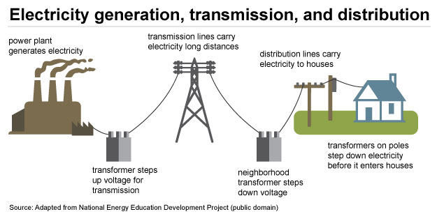
This is a flowchart. Power plant generation > transformer which steps up voltage for transmission > transmission lines carry electricity long distances > neighborhood transformer steps down voltage > distribution lines carry electricity to houses > transformers on poles step down electricity before it enters houses.
Prior to the process of electricity restructuring, the primary players in the electric power business in the United States were vertically integrated utilities and their state regulators.
Electricity reforms in the United States began in the 1990s. Not all states elected to reform their electric utilities, but most of the states in the northeastern U.S., along with California and Texas, did choose to reform and restructure the electric utility business. Most states in the southern and western US did not choose to undertake electric utility reforms and still have vertically integrated utilities with tight state regulation.
Broadly, the process of electricity reform (sometimes called "deregulation" and sometimes called "restructuring") consisted of the following:
-
The vertically integrated electric utility was broken up into three separate companies - one each for generation, transmission, and distribution. Oftentimes, the same parent company owned all three businesses as independent subsidiaries.
-
Price regulation on power generation was removed or substantially loosened. Rather than charging regulated prices, power generation companies could charge whatever price the market would bear. These new electricity markets would be regulated by the Federal Energy Regulatory Commission rather than by the individual states.
-
Electric transmission would mostly retain its regulated pricing, but much responsibility for setting transmission prices was shifted away from the states, into the hands of the Federal Energy Regulatory Commission.
-
Some financing processes for power plants were loosened, allowing for faster accounting depreciation of new equipment.
The process of electricity reform has dramatically widened the number of types of companies and regulatory agencies involved in electricity supply.
Regional Transmission Organizations (RTOs)
Regional Transmission Organizations (RTOs) are non-profit, public-benefit corporations that were created as a part of electricity restructuring in the United States, beginning in the 1990s. Some RTOs, such as PJM in the Mid-Atlantic states, were created from existing “power pools” dating back many decades (PJM was first organized in the 1920s). RTOs are regulated by FERC, not by the states. There are seven RTOs in the U.S., covering about half of the states' and roughly two-thirds of total U.S.'s annual electricity demand. Each RTO establishes its own rules and market structures, but there are many commonalities. Broadly, the RTO performs the following functions:
- management of the bulk power transmission system within its footprint;
- ensuring non-discriminatory access to the transmission grid by customers and suppliers;
- dispatch of generation assets within its footprint to keep supply and demand in balance;
- regional planning for generation and transmission (see below for limitations to this function);
- with the exception of the Southwest Power Pool (SPP), RTOs also run a number of markets for electric generation service.
RTOs have responsibility for ensuring reliability and adequacy of the power grid. They must perform regional planning, meaning that they determine where additional power lines and generators are required in order to maintain system reliability.
Uniform Price Auction
Uniform Price Auctions
Virtually all RTO markets are operated as “uniform price auctions.” Under the uniform price auction, generators submit supply offers to the RTO, and the RTO chooses the lowest-cost supply offers until supply is equal to the RTO’s demand. This process is called “clearing the market.” The last generator dispatched is called the “marginal unit” and sets the market price. Any generator whose supply offer is below the market-clearing price is said to have “cleared the market,” and is paid the market-clearing price for the amount of supply that cleared the market. Generators with marginal operating costs below the market-clearing price will earn profits. In general, if the market is competitive (all suppliers offer at marginal operating cost) the marginal unit does not earn any profit.
As a reminder of how this system works, the uniform price auction is illustrated in Figure 12.1. There are five suppliers, each of which offers its capacity to the market at a different price. These supply offers are shown in Table 12.1. Here we will assume that supply offers are equal to the marginal costs of each generator, but in the deregulated generation market suppliers are not really obligated to submit offers that are equal to costs. The RTO aggregates these supply offers to form a single market-wide “dispatch stack” or supply curve. Demand is represented by a vertical line (the RTO assumes that demand is fixed, or “perfectly inelastic” with respect to price). In this case, demand is 55 MWh. Generators A, B, C, and D clear the market. Generator E does not clear the market since its supply offer is too high. The market-clearing price, known as the “system marginal price (SMP)” would be $40 per MWh. Generators A, B, C, and D would each be paid $40 per MWh. Generators A, B and C would earn a profit. Generator D is the marginal unit, so it earns zero profit.
| Supplier | Capacity (MW) |
Marginal cost ($/MWh) |
|---|---|---|
| A | 10 | $10 |
| B | 15 | $15 |
| C | 20 | $30 |
| D | 25 | $40 |
| E | 10 | $70 |
Each generator that clears the market (in this case, it would be A, B, C, and D; E does not clear the market) earns the SMP for each unit of electricity they sell. Total hourly profits are thus calculated as:
Profit = Output × (SMP – Marginal Cost).
Since the SMP in our example is equal to $40, hourly profits are calculated as:
Note in particular that Firm D, which is the “marginal unit” setting the SMP of $40/MWh, clears the market but does not earn any profits.
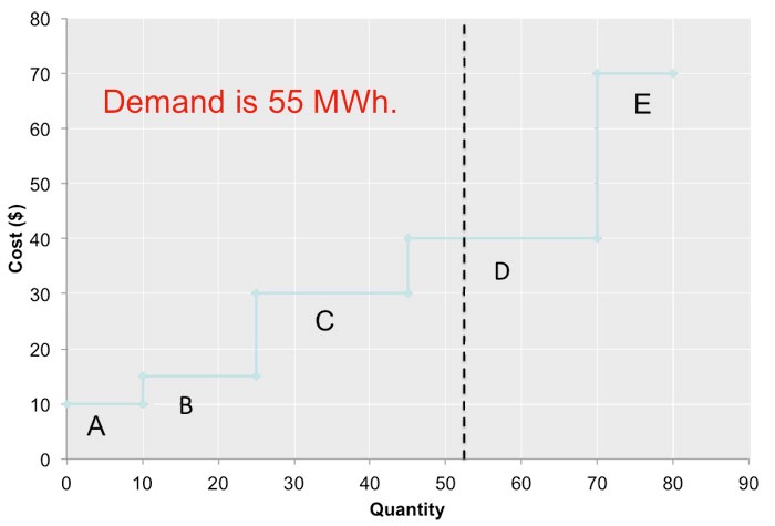
Locational Marginal Pricing
In the previous page, we learned how the uniform price auction works: Generators submit supply offers; the RTO aggregates those supply offers to form a system supply curve or "dispatch curve;" and the market clears at the point where the dispatch curve intersects the (fixed) level of demand. Those generators with supply offers below the market clearing point are dispatched, while those with supply offers above the market clearing point are not dispatched.
In the absence of any transmission congestion, every generator clearing the market would get paid the SMP. This is why low cost generators, which we call "inframarginal suppliers," can be very profitable, and the marginal generator earns no profit under the uniform price auction.
When there is transmission congestion, however, things get more complicated because the transmission congestion segments the market. Some areas of the market are on one side of the constraint and some areas are on the other side of the constraint, and no further deliveries can take place between the two areas. If demand increases on one side of the constraint, a generator on that side of the constraint has to be dispatched to meet that demand. If demand increases on the other side of the constraint, a different generator on that side of the constraint has to be dispatched. These generators may have different costs and supply offers, and thus the marginal cost of meeting demand in one location is different from the marginal cost of meeting demand in another location. These location-specific costs are called Locational Marginal Prices.
The formal definition is that the Locational Marginal Price (LMP) at some node k in the network is the marginal cost to the RTO of delivering an additional unit of energy to node k. Relatedly, we sometimes define the "transmission price" or "congestion cost" between two nodes j and k in the network as the difference in LMPs between the two nodes.
The LMP forms the basis for payments to generators and payments by buyers in the PJM electricity market and other such markets in the US. Generators are paid the LMP at their node for electric energy produced, and buyers pay the LMP at their node for electric energy consumed. The RTO acts as the middleman for all purchases and sales, so it collects money from buyers and pays money to sellers.
If there is no transmission congestion in the network, then LMPs at all nodes are equal and will be equal to the System Marginal Price (SMP). This says that if no transmission lines are constrained, then the same marginal generator could be used to serve an additional unit of electric energy demand anywhere in the network.
LMPs can be highly variable across different parts of an RTO territory and can be very volatile depending on system conditions. The figure below shows a heat map of LMPs in the PJM system on a warm, but not terribly hot, summer day. The areas in blue (in the western part of the PJM territory) have very low LMPs, indicating that there is a lot of low-cost generation capacity in those regions to meet demand. The areas in yellow and red exhibit higher LMPs, while the area around Washington, DC has the highest LMPs (in white). Why does this happen? The answer is that there are transmission constraints in the PJM network that limit the amount of low-cost generation in places like Ohio that can be used to meet high electricity demand in places like Washington, DC. There is plenty of generation but not enough transmission to move the power around. So to meet electricity demand in Washington, DC, PJM must use higher-cost generators that are located closer to Washington, DC.
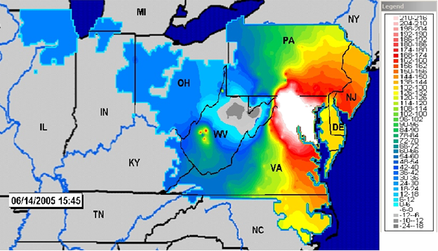
Note that electricity demand is highly variable over time. Consequently, in addition to the high variability over the space, LMPs can also be highly variable over time.
Temporal and Locational risks
Earlier in this lesson, we discussed transmission congestion and Locational Marginal Prices. As you can see in Figure 2. LMPs are highly volatile. They are calculated at thousands of different locations and change almost constantly. You may also notice that the difference between LMPs at various locations is also volatile. Sometimes the price at one node is higher than at another node, and sometimes it is lower.
We generally define two dimensions of risk in electricity markets: temporal risk and locational or "basis" risk.
Temporal Risk
Temporal risk pertains to volatility in the LMP at a specific location over time; Risk associated with variation in a node or zone of prices over time. Temporal risk arises due to changes in electricity demand and fuel prices at a specific location.
Locational or "Basis" Risk
Locational or "basis" risk pertains to volatility in the LMP across space (between two or more locations); Risk associated with variation of the transmission price between two nodes or zones. This is the same thing as variation in the difference between two LMPs or zonal prices. Locational risk is sometimes referred to as “basis risk” in the electricity industry.
These two types of risk may need to be managed through various hedging instruments, but they also may represent arbitrage opportunities.
Two of the most common ways of exercising arbitrage in electricity markets are through "virtual bidding" (arbitraging the difference between the clearing price in the day-ahead and real-time electricity market) and through the "spark spread" (the difference between fuel and electricity prices).
Virtual Bidding
Virtual bidding offers a mechanism for electricity market participants to take advantage of differences between day-ahead and real-time prices at a specific location. It involves buying or selling some quantity of electricity in the day-ahead market, and then taking an offsetting position in the real-time market. Large financial institutions like investment banks and hedge funds engage in a lot of virtual bidding, but other types of market participants like generating companies and electric utilities also engage in virtual bidding. The mechanics of virtual bidding are very simple. A market participant first takes a short or long position in the day-ahead market. A short position is known as a "dec" and a long position is known as an "inc." If that market participant's inc or dec clears the day-ahead market (in other words, if that participant would get dispatched if it represented an actual physical need to buy or sell electricity), then the market participant must take an offsetting position in the real-time market. So, a day-ahead dec would be paired with a real-time inc, and a day-ahead inc would be paired with a real-time dec. The quantities offset one another and in the end, the market participant does not have to buy or sell any actual electricity. But the market participant is paid the LMP for the inc and pays the LMP for the dec.
For example, a market participant submits a 1 MW inc in the day-ahead market, believing that the day-ahead price will be greater than the real-time price. We'll say that the inc clears the market and the day-ahead LMP is $25/MWh. This same market participant would submit a dec to the real-time market, and we'll say that the dec clears the real-time market and the real-time price is $20/MWh. What has basically happened is that this market participant has sold 1 MWh of energy at $25/MWh and bought that same MWh for $20, netting $5 in profit.
Spark Spread
The second mechanism for exercising arbitrage is through the "spark spread," which is the difference between the electricity price and the cost of generating electricity, which is mainly the fuel cost. The arbitrage opportunity that the spark spread represents is typically the opportunity to buy fuel and sell electricity. Spark spreads in financial markets are typically defined as the difference between the LMP and the cost of producing electricity by a natural gas generator with certain characteristics (like a heat rate of 10,000 and variable O&M costs of $2.50 per MWh).
As an example, let's say that the electricity price is $100/MWh and the cost of fuel is $5 per million BTU. The marginal cost of a gas-fired generator at this fuel price with a heat rate of 10 million BTU/MWh and variable O&M costs of $2.50/MWh would be 10*5 + 2.50 = $52.50/MWh. The spark spread would thus be $100/MWh - $52.50/MWh = $47.50/MWh.
The figure below shows some historical LMPs in PJM as compared to our hypothetical gas generation marginal cost of $52.50/MWh. During some hours, the spark spread is negative, indicating that it would not be profitable to buy fuel and sell electricity. During other hours, the spark spread is positive, indicating that it would be profitable to buy fuel and sell electricity.
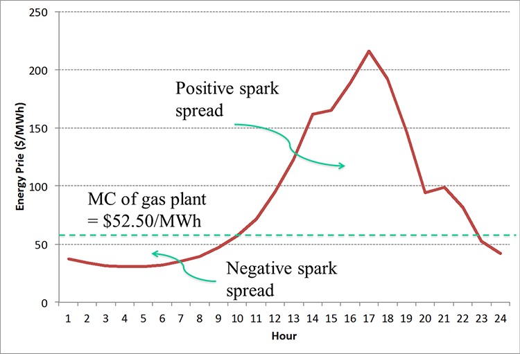
Financial Transmission Rights and Contracts for Differences
Now we will see how locational and temporal risk can be hedged in electricity markets.
Financial Transmission Rights
Financial Transmission Rights (FTRs) are financial instruments that entitle the holder to the difference between LMPs at two defined locations (any two points a and b on the grid). The parameters for an FTR are:
- A "source" node, which we will call node a.
- A "sink" node, which we will call node b.
- A quantity, in MW, which we will call M.
Note that the points do not need to be connected neighbors.
The holder of an M megawatt FTR from a to b at time t receives
FTRs are typically auctioned off quarterly by the RTO, and may have different durations (one-month FTRs versus quarterly FTRs, for example) and market participants bid for quantities, source nodes, and sink nodes. Most FTRs are structured as obligations, which means FTR gives the holder the difference, LMP(sink) – LMP(source). If LMPb > LMPa then the holder of the FTR is paid money by the RTO. If LMPb < LMPa then the holder of the FTR must pay the RTO.
Some FTRs may be structured as options that renew every hour, in which case during a given hour the FTR holder would choose to exercise the option only if LMPb > LMPa, i.e. If the payoff would be positive. The payoff from an M-megawatt FTR option from node a to node b would thus be:
FTRs also obey superposition, just like power flows. An M-megawatt FTR defined from a to b and an M-megawatt FTR from b to a will cancel each other out financially (as long as both FTRs are structured as obligations). An M-megawatt FTR from a to b and an M-2 megawatt FTR from b to a would have identical value as a 2 megawatt FTR from a to b.
As financial instruments, FTRs are very similar to swaps. A swap is an agreement to exchange the closing price of two different financial assets. In this case, the "swap" is between two nodes in the power network, not between two different financial assets.
Contracts for Differences
In conventional financial market analysis, a contract for differences (CFD) is an agreement to exchange the opening and closing prices of some financial asset. In electricity markets, a CFD is a bilateral agreement in which one party gets a fixed price for electric energy (the strike price) plus an adjustment to cover the difference between the strike price and the spot price. This adjustment may be a positive or negative number.
CFDs are different than FTRs in two ways. First, a CFD is usually defined at a specific location, not between a pair of locations. Thus, CFDs are a tool principally for hedging temporal price risk - the variation in the LMP over time at a specific location. Second, CFDs are not traded through RTO markets. They are bilateral contracts between individual market participants.
CFDs may be defined as "one-way" or "two-way" contracts. A one-way CFD can have a couple of different payment mechanisms. First, a one-way CFD can be structured so that if the spot price exceeds the strike price, the seller pays the buyer the difference. Otherwise, there are no side payments. Second, a one-way CFD can be structured so that if the strike price exceeds the spot price, the buyer pays the seller the difference. Otherwise, there are no side payments.
A two-way CFD is just the sum of two one-way CFDs and is basically a forward contract for electric energy. In a two-way CFD, the seller pays the buyer if the spot price exceeds the strike price; and the buyer pays the seller if the strike price exceeds the spot price.
Here is an example. Let's say that a generation company signs a 100 MWh one-way CFD with an electricity consumer. The strike price is $50/MWh, and the CFD is defined at the location of the consumer.
Let's first say that the LMP at the location of the consumer is $75/MWh. In this case, the generator would earn $50*100 = $5,000 in revenue from the CFD, but would then need to pay the consumer 100*($75-$50) = $2,500 under the terms of the CFD. So the generator's net CFD revenue would be $2,500.
Now, let's say that the LMP at the location of the consumer is $40/MWh. In this case, there are no side payments and the generator's CFD revenues are $5,000.
Hedging with FTRs and CFDs
Thus far, we have seen that temporal risk can be hedged with Contracts for Differences. A one way CFD can basically put a ceiling on the price of electricity. A two-way CFD is essentially identical to a forward contract for electricity at a fixed price. Locational risk can be hedged with Financial Transmission Rights.
In this section, we will see how a combination of CFDs and FTRs can be used to create a "perfect hedge" that shifts all temporal and locational risk. The end result of this perfect hedge is like a fixed-price contract at the strike price of the CFD, as long as the quantities of the CFD and FTR are equal to the amount of power being transferred from the source node to the sink node.
The table below outlines the perfect hedging model. We'll assume that there is a supplier located at node a, and a consumer located at node b. The supplier produces Q MWh in the real-time market and the consumer uses Q MWh. We will let F denote the size of a two-way CFD defined at the customer's node, and M denote the size of the FTR held by the supplier. The FTR is defined such that node a is the source and node b is the sink.
| Mechanism | Payment to Supplier at node a | Payment by consumer at node b |
|---|---|---|
| Spot Market | ||
|
F Megawatt Two-Way CFD at strike price p |
||
| Total | ||
|
M Megawatt FTR from node a to node b |
-- | |
| Total if F = M | ||
| Total if F = M = Q |
Let's walk through the rows of the table:
- The first row shows the spot market revenues and costs for the supplier and consumer.
- The second row shows the payments under the CFD, assuming the strike price is equal to p. Note that if the LMP at node b exceeds p, the generator pays the consumer the difference. If the LMP at node b is smaller than p, the consumer pays the generator.
- The third row shows the sum of payments to the supplier and payments by the consumer from the real-time energy market and the CFD.
- The fourth row shows the FTR payment. This is zero for the consumer because the supplier is assumed to hold the FTR.
- The fifth row shows the total payments for the supplier and consumer if the FTR is the same size as the CFD. Note that because of the CFD defined at node b, and because of the FTR, any payments involving the LMP at node b cancel each other out. This is because the payment stream for the supplier from the FTR and CFD move in opposite directions.
- The sixth row shows the total payments if the FTR, CFD and amount of physical production/consumption at nodes a and b are identical. In this case, all LMP terms cancel out. The supplier is paid the LMP at node a through the real-time market and pays the LMP at node a through the FTR. The consumer pays the LMP at node b and then is paid the difference between the LMP at node b and the CFD strike price p. All that is left is that the supplier earns revenue equal to the CFD strike price times output, while the consumer pays the same amount.
Note that unlike other energy commodities, electricity transportation cost is highly variable. Thus, due to the temporal and locational risks (high volatility over space and time), NYMEX futures contracts [137] don’t add much value to the market, and they are not popular, or the traded volume is very low. Consequently, it’s more efficient to use the mentioned financial instruments and utilize them for the spot market.
Summary and Final Tasks
Key Learning Points: Lesson 12
- Since electricity cannot be stored in large volumes at a reasonable cost, supply and demand has to balance at every moment.
- Unlike transportation cost in the oil and gas market, electricity transmission cost is highly volatile.
- Prior to the process of electricity restructuring, the primary players in the electric power business in the United States were vertically integrated utilities and their state regulators.
- Regional Transmission Organizations (RTOs) have responsibility for ensuring reliability and adequacy of the power grid.
- Under the uniform price auction, generators submit supply offers to the RTO, and the RTO chooses the lowest-cost supply offers until supply is equal to the RTO’s demand.
- Locational Marginal Price (LMP) at some node k in the network is the marginal cost to the RTO of delivering an additional unit of energy to node k.
- We generally define two dimensions of risk in electricity markets: temporal risk and locational or "basis" risk.
- Temporal risk pertains to volatility in the LMP at a specific location over time.
- Locational or "basis" risk pertains to volatility in the LMP across space (between two or more locations)
- Two of the most common ways of exercising arbitrage in electricity markets are through:
- "virtual bidding“: arbitraging the difference between the clearing price in the day-ahead and real-time electricity market
- "spark spread“: the difference between fuel and electricity prices
- Locational and temporal risk in electricity markets can be hedged through:
- Financial Transmission Rights (FTR): financial instruments that entitle the holder to the difference between LMPs at two defined locations
- Contracts for Differences (CFD): a bilateral agreement in which one party gets a fixed price for electric energy (the strike price) plus an adjustment to cover the difference between the strike price and the spot price.
- A combination of CFDs and FTRs can be used to create a "perfect hedge" that shifts all temporal and locational risk.
Reminder - Complete all of the Lesson 12 tasks!
You have reached the end of Lesson 12. Double-check the list of requirements on the first page of this lesson to make sure you have completed all of the activities listed there before beginning the next lesson.