Lesson 12: Risk Management in the Electricity Market
Lesson 12 Introduction
Overview
This lesson will focus on the electricity market and introduce the major players and common financial instruments in the market. Since electricity cannot be stored in large volumes at a reasonable cost, part of the job of the power grid operator is to make sure that supply and demand balance at every moment. This means that the power grid is making adjustments every single second (or less than a second) as demand changes. Many of these adjustments are automated responses. This gives unique characteristics to the electricity market that is not common in other energy markets. Unlike transportation cost in the oil and gas market, electricity transmission cost is highly volatile. Because of these characteristics, NYMEX futures contracts don’t add much value to the market, and they are not commonly traded, or the traded volume is very low. Consequently, other financial instruments are being used for the purposes of arbitrage and hedging.
We will learn what is called the "energy market" portion of the PJM market model. The energy market is essentially a set of two connected short-term forward markets. The first, called the "day ahead" market, commits generators to be able to produce electricity 24 hours in advance, based on forecasted demand. The second, called the "real-time" market or "hour ahead" market, commits generators to be able to produce electricity one hour in advance, based on an updated demand forecast. You can think about the day-ahead market as setting a schedule of which power plants should be available to produce energy, while the real-time market shifts those schedules around a little bit based on an improved forecast of electricity demand.
Learning Outcomes
At the successful completion of this lesson, students should be able to:
- explain the basics of the electricity market and its differences comparing to other energy commodity markets;
- outline electricity market reform;
- define the RTO’s role in the electricity market;
- describe the uniform price auction mechanism;
- be able to recognize the temporal and locational risks in the electricity market;
- demonstrate the financial instruments being used for arbitrage and hedging purposes:
- virtual bidding,
- spark spread,
- financial transmission rights,
- contracts for differences.
What is due for Lesson 12?
This lesson will take us one week to complete. The following items will be due Sunday at 11:59 p.m. Eastern Time.
- Lesson 12 Quiz
- Lesson 12 activities as assigned in Canvas
Questions?
If you have any questions, please post them to our General Course Questions discussion forum (not email), located under Modules in Canvas. The TA and I will check that discussion forum daily to respond. While you are there, feel free to post your own responses if you, too, are able to help out a classmate.
Note
The majority of this lesson was modified, with permission, from Penn State's EBF 483, Introduction to Electricity Markets written by Dr. Seth Blumsack.
Reading Assignment: Lesson 12
Required Readings
Please read the following pages from the U.S. Energy Information Administration.
Optional Readings
Uses of Electricity
Prices and Factors Affecting Prices
Basics of the Electricity Market
Electric power in the United States is a $350 billion per year business and touches literally every corner of the economy. The "power grid" in North America is massive in scale and scope.
The figure below shows the three segments of the electricity supply chain - generation, transmission, and distribution. For nearly a century in the United States, there was one type of vertically integrated company performing all three of these functions. This company, called the "electric utility," generated its own electricity, moved that electricity over its own transmission lines within its geographic service area, and then delivered the power to its customers using its distribution lines. The electric utility usually had its prices, investments, and business practices tightly regulated by individual states. The federal government in the United States did not have a dominant role in the electric utility business until the process of deregulation and reorganization began in the 1990s.
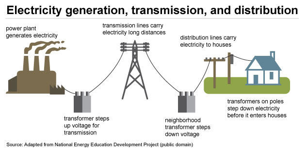
This is a flowchart. Power plant generation > transformer which steps up voltage for transmission > transmission lines carry electricity long distances > neighborhood transformer steps down voltage > distribution lines carry electricity to houses > transformers on poles step down electricity before it enters houses.
Prior to the process of electricity restructuring, the primary players in the electric power business in the United States were vertically integrated utilities and their state regulators.
Electricity reforms in the United States began in the 1990s. Not all states elected to reform their electric utilities, but most of the states in the northeastern U.S., along with California and Texas, did choose to reform and restructure the electric utility business. Most states in the southern and western US did not choose to undertake electric utility reforms and still have vertically integrated utilities with tight state regulation.
Broadly, the process of electricity reform (sometimes called "deregulation" and sometimes called "restructuring") consisted of the following:
-
The vertically integrated electric utility was broken up into three separate companies - one each for generation, transmission, and distribution. Oftentimes, the same parent company owned all three businesses as independent subsidiaries.
-
Price regulation on power generation was removed or substantially loosened. Rather than charging regulated prices, power generation companies could charge whatever price the market would bear. These new electricity markets would be regulated by the Federal Energy Regulatory Commission rather than by the individual states.
-
Electric transmission would mostly retain its regulated pricing, but much responsibility for setting transmission prices was shifted away from the states, into the hands of the Federal Energy Regulatory Commission.
-
Some financing processes for power plants were loosened, allowing for faster accounting depreciation of new equipment.
The process of electricity reform has dramatically widened the number of types of companies and regulatory agencies involved in electricity supply.
Regional Transmission Organizations (RTOs)
Regional Transmission Organizations (RTOs) are non-profit, public-benefit corporations that were created as a part of electricity restructuring in the United States, beginning in the 1990s. Some RTOs, such as PJM in the Mid-Atlantic states, were created from existing “power pools” dating back many decades (PJM was first organized in the 1920s). RTOs are regulated by FERC, not by the states. There are seven RTOs in the U.S., covering about half of the states' and roughly two-thirds of total U.S.'s annual electricity demand. Each RTO establishes its own rules and market structures, but there are many commonalities. Broadly, the RTO performs the following functions:
- management of the bulk power transmission system within its footprint;
- ensuring non-discriminatory access to the transmission grid by customers and suppliers;
- dispatch of generation assets within its footprint to keep supply and demand in balance;
- regional planning for generation and transmission (see below for limitations to this function);
- with the exception of the Southwest Power Pool (SPP), RTOs also run a number of markets for electric generation service.
RTOs have responsibility for ensuring reliability and adequacy of the power grid. They must perform regional planning, meaning that they determine where additional power lines and generators are required in order to maintain system reliability.
Uniform Price Auction
Uniform Price Auctions
Virtually all RTO markets are operated as “uniform price auctions.” Under the uniform price auction, generators submit supply offers to the RTO, and the RTO chooses the lowest-cost supply offers until supply is equal to the RTO’s demand. This process is called “clearing the market.” The last generator dispatched is called the “marginal unit” and sets the market price. Any generator whose supply offer is below the market-clearing price is said to have “cleared the market,” and is paid the market-clearing price for the amount of supply that cleared the market. Generators with marginal operating costs below the market-clearing price will earn profits. In general, if the market is competitive (all suppliers offer at marginal operating cost) the marginal unit does not earn any profit.
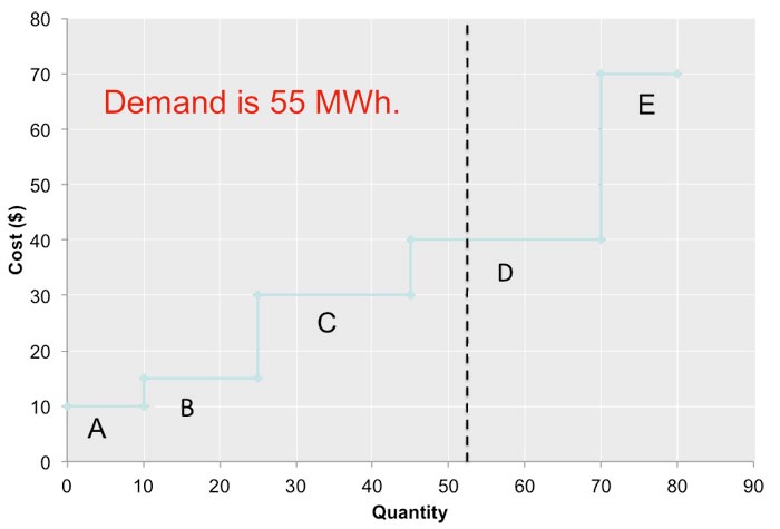
As a reminder of how this system works, the uniform price auction is illustrated in Figure 12.1. There are five suppliers, each of which offers its capacity to the market at a different price. These supply offers are shown in Table 12.1. Here we will assume that supply offers are equal to the marginal costs of each generator, but in the deregulated generation market suppliers are not really obligated to submit offers that are equal to costs. The RTO aggregates these supply offers to form a single market-wide “dispatch stack” or supply curve. Demand is represented by a vertical line (the RTO assumes that demand is fixed, or “perfectly inelastic” with respect to price). In this case, demand is 55 MWh. Generators A, B, C, and D clear the market. Generator E does not clear the market since its supply offer is too high. The market-clearing price, known as the “system marginal price (SMP)” would be $40 per MWh. Generators A, B, C, and D would each be paid $40 per MWh. Generators A, B and C would earn a profit. Generator D is the marginal unit, so it earns zero profit.
| Supplier | Capacity (MW) |
Marginal cost ($/MWh) |
|---|---|---|
| A | 10 | $10 |
| B | 15 | $15 |
| C | 20 | $30 |
| D | 25 | $40 |
| E | 10 | $70 |
Each generator that clears the market (in this case, it would be A, B, C, and D; E does not clear the market) earns the SMP for each unit of electricity they sell. Total hourly profits are thus calculated as:
Profit = Output × (SMP – Marginal Cost).
Since the SMP in our example is equal to $40, hourly profits are calculated as:
Note in particular that Firm D, which is the “marginal unit” setting the SMP of $40/MWh, clears the market but does not earn any profits.
Locational Marginal Pricing
In the previous page, we learned how the uniform price auction works: Generators submit supply offers; the RTO aggregates those supply offers to form a system supply curve or "dispatch curve;" and the market clears at the point where the dispatch curve intersects the (fixed) level of demand. Those generators with supply offers below the market clearing point are dispatched, while those with supply offers above the market clearing point are not dispatched.
In the absence of any transmission congestion, every generator clearing the market would get paid the SMP. This is why low cost generators, which we call "inframarginal suppliers," can be very profitable, and the marginal generator earns no profit under the uniform price auction.
When there is transmission congestion, however, things get more complicated because the transmission congestion segments the market. Some areas of the market are on one side of the constraint and some areas are on the other side of the constraint, and no further deliveries can take place between the two areas. If demand increases on one side of the constraint, a generator on that side of the constraint has to be dispatched to meet that demand. If demand increases on the other side of the constraint, a different generator on that side of the constraint has to be dispatched. These generators may have different costs and supply offers, and thus the marginal cost of meeting demand in one location is different from the marginal cost of meeting demand in another location. These location-specific costs are called Locational Marginal Prices.
The formal definition is that the Locational Marginal Price (LMP) at some node k in the network is the marginal cost to the RTO of delivering an additional unit of energy to node k. Relatedly, we sometimes define the "transmission price" or "congestion cost" between two nodes j and k in the network as the difference in LMPs between the two nodes.
The LMP forms the basis for payments to generators and payments by buyers in the PJM electricity market and other such markets in the US. Generators are paid the LMP at their node for electric energy produced, and buyers pay the LMP at their node for electric energy consumed. The RTO acts as the middleman for all purchases and sales, so it collects money from buyers and pays money to sellers.
If there is no transmission congestion in the network, then LMPs at all nodes are equal and will be equal to the System Marginal Price (SMP). This says that if no transmission lines are constrained, then the same marginal generator could be used to serve an additional unit of electric energy demand anywhere in the network.
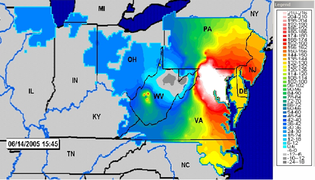
LMPs can be highly variable across different parts of an RTO territory and can be very volatile depending on system conditions. The figure below shows a heat map of LMPs in the PJM system on a warm, but not terribly hot, summer day. The areas in blue (in the western part of the PJM territory) have very low LMPs, indicating that there is a lot of low-cost generation capacity in those regions to meet demand. The areas in yellow and red exhibit higher LMPs, while the area around Washington, DC has the highest LMPs (in white). Why does this happen? The answer is that there are transmission constraints in the PJM network that limit the amount of low-cost generation in places like Ohio that can be used to meet high electricity demand in places like Washington, DC. There is plenty of generation but not enough transmission to move the power around. So to meet electricity demand in Washington, DC, PJM must use higher-cost generators that are located closer to Washington, DC.
Note that electricity demand is highly variable over time. Consequently, in addition to the high variability over the space, LMPs can also be highly variable over time.
Temporal and Locational risks
Earlier in this lesson, we discussed transmission congestion and Locational Marginal Prices. As you can see in Figure 2. LMPs are highly volatile. They are calculated at thousands of different locations and change almost constantly. You may also notice that the difference between LMPs at various locations is also volatile. Sometimes the price at one node is higher than at another node, and sometimes it is lower.
We generally define two dimensions of risk in electricity markets: temporal risk and locational or "basis" risk.
Temporal Risk
Temporal risk pertains to volatility in the LMP at a specific location over time; Risk associated with variation in a node or zone of prices over time. Temporal risk arises due to changes in electricity demand and fuel prices at a specific location.
Locational or "Basis" Risk
Locational or "basis" risk pertains to volatility in the LMP across space (between two or more locations); Risk associated with variation of the transmission price between two nodes or zones. This is the same thing as variation in the difference between two LMPs or zonal prices. Locational risk is sometimes referred to as “basis risk” in the electricity industry.
These two types of risk may need to be managed through various hedging instruments, but they also may represent arbitrage opportunities.
Two of the most common ways of exercising arbitrage in electricity markets are through "virtual bidding" (arbitraging the difference between the clearing price in the day-ahead and real-time electricity market) and through the "spark spread" (the difference between fuel and electricity prices).
Virtual Bidding
Virtual bidding offers a mechanism for electricity market participants to take advantage of differences between day-ahead and real-time prices at a specific location. It involves buying or selling some quantity of electricity in the day-ahead market, and then taking an offsetting position in the real-time market. Large financial institutions like investment banks and hedge funds engage in a lot of virtual bidding, but other types of market participants like generating companies and electric utilities also engage in virtual bidding. The mechanics of virtual bidding are very simple. A market participant first takes a short or long position in the day-ahead market. A short position is known as a "dec" and a long position is known as an "inc." If that market participant's inc or dec clears the day-ahead market (in other words, if that participant would get dispatched if it represented an actual physical need to buy or sell electricity), then the market participant must take an offsetting position in the real-time market. So, a day-ahead dec would be paired with a real-time inc, and a day-ahead inc would be paired with a real-time dec. The quantities offset one another and in the end, the market participant does not have to buy or sell any actual electricity. But the market participant is paid the LMP for the inc and pays the LMP for the dec.
For example, a market participant submits a 1 MW inc in the day-ahead market, believing that the day-ahead price will be greater than the real-time price. We'll say that the inc clears the market and the day-ahead LMP is $25/MWh. This same market participant would submit a dec to the real-time market, and we'll say that the dec clears the real-time market and the real-time price is $20/MWh. What has basically happened is that this market participant has sold 1 MWh of energy at $25/MWh and bought that same MWh for $20, netting $5 in profit.
Spark Spread
The second mechanism for exercising arbitrage is through the "spark spread," which is the difference between the electricity price and the cost of generating electricity, which is mainly the fuel cost. The arbitrage opportunity that the spark spread represents is typically the opportunity to buy fuel and sell electricity. Spark spreads in financial markets are typically defined as the difference between the LMP and the cost of producing electricity by a natural gas generator with certain characteristics (like a heat rate of 10,000 and variable O&M costs of $2.50 per MWh).
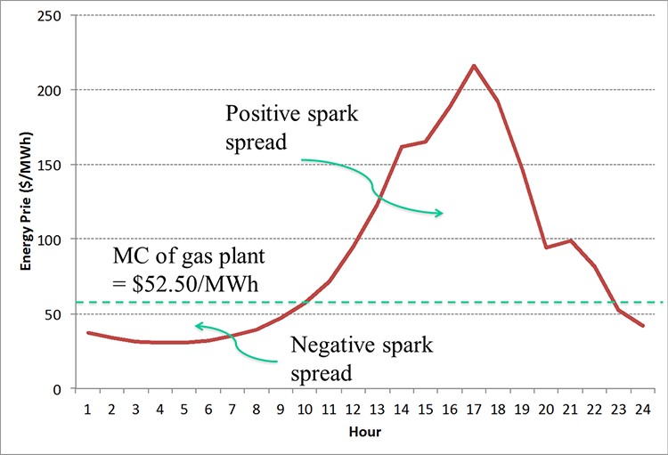
As an example, let's say that the electricity price is $100/MWh and the cost of fuel is $5 per million BTU. The marginal cost of a gas-fired generator at this fuel price with a heat rate of 10 million BTU/MWh and variable O&M costs of $2.50/MWh would be 10*5 + 2.50 = $52.50/MWh. The spark spread would thus be $100/MWh - $52.50/MWh = $47.50/MWh.
The figure below shows some historical LMPs in PJM as compared to our hypothetical gas generation marginal cost of $52.50/MWh. During some hours, the spark spread is negative, indicating that it would not be profitable to buy fuel and sell electricity. During other hours, the spark spread is positive, indicating that it would be profitable to buy fuel and sell electricity.
Financial Transmission Rights and Contracts for Differences
Now we will see how locational and temporal risk can be hedged in electricity markets.
Financial Transmission Rights
Financial Transmission Rights (FTRs) are financial instruments that entitle the holder to the difference between LMPs at two defined locations (any two points a and b on the grid). The parameters for an FTR are:
- A "source" node, which we will call node a.
- A "sink" node, which we will call node b.
- A quantity, in MW, which we will call M.
Note that the points do not need to be connected neighbors.
The holder of an M megawatt FTR from a to b at time t receives
FTRs are typically auctioned off quarterly by the RTO, and may have different durations (one-month FTRs versus quarterly FTRs, for example) and market participants bid for quantities, source nodes, and sink nodes. Most FTRs are structured as obligations, which means FTR gives the holder the difference, LMP(sink) – LMP(source). If LMPb > LMPa then the holder of the FTR is paid money by the RTO. If LMPb < LMPa then the holder of the FTR must pay the RTO.
Some FTRs may be structured as options that renew every hour, in which case during a given hour the FTR holder would choose to exercise the option only if LMPb > LMPa, i.e. If the payoff would be positive. The payoff from an M-megawatt FTR option from node a to node b would thus be:
FTRs also obey superposition, just like power flows. An M-megawatt FTR defined from a to b and an M-megawatt FTR from b to a will cancel each other out financially (as long as both FTRs are structured as obligations). An M-megawatt FTR from a to b and an M-2 megawatt FTR from b to a would have identical value as a 2 megawatt FTR from a to b.
As financial instruments, FTRs are very similar to swaps. A swap is an agreement to exchange the closing price of two different financial assets. In this case, the "swap" is between two nodes in the power network, not between two different financial assets.
Contracts for Differences
In conventional financial market analysis, a contract for differences (CFD) is an agreement to exchange the opening and closing prices of some financial asset. In electricity markets, a CFD is a bilateral agreement in which one party gets a fixed price for electric energy (the strike price) plus an adjustment to cover the difference between the strike price and the spot price. This adjustment may be a positive or negative number.
CFDs are different than FTRs in two ways. First, a CFD is usually defined at a specific location, not between a pair of locations. Thus, CFDs are a tool principally for hedging temporal price risk - the variation in the LMP over time at a specific location. Second, CFDs are not traded through RTO markets. They are bilateral contracts between individual market participants.
CFDs may be defined as "one-way" or "two-way" contracts. A one-way CFD can have a couple of different payment mechanisms. First, a one-way CFD can be structured so that if the spot price exceeds the strike price, the seller pays the buyer the difference. Otherwise, there are no side payments. Second, a one-way CFD can be structured so that if the strike price exceeds the spot price, the buyer pays the seller the difference. Otherwise, there are no side payments.
A two-way CFD is just the sum of two one-way CFDs and is basically a forward contract for electric energy. In a two-way CFD, the seller pays the buyer if the spot price exceeds the strike price; and the buyer pays the seller if the strike price exceeds the spot price.
Here is an example. Let's say that a generation company signs a 100 MWh one-way CFD with an electricity consumer. The strike price is $50/MWh, and the CFD is defined at the location of the consumer.
Let's first say that the LMP at the location of the consumer is $75/MWh. In this case, the generator would earn $50*100 = $5,000 in revenue from the CFD, but would then need to pay the consumer 100*($75-$50) = $2,500 under the terms of the CFD. So the generator's net CFD revenue would be $2,500.
Now, let's say that the LMP at the location of the consumer is $40/MWh. In this case, there are no side payments and the generator's CFD revenues are $5,000.
Hedging with FTRs and CFDs
Thus far, we have seen that temporal risk can be hedged with Contracts for Differences. A one way CFD can basically put a ceiling on the price of electricity. A two-way CFD is essentially identical to a forward contract for electricity at a fixed price. Locational risk can be hedged with Financial Transmission Rights.
In this section, we will see how a combination of CFDs and FTRs can be used to create a "perfect hedge" that shifts all temporal and locational risk. The end result of this perfect hedge is like a fixed-price contract at the strike price of the CFD, as long as the quantities of the CFD and FTR are equal to the amount of power being transferred from the source node to the sink node.
The table below outlines the perfect hedging model. We'll assume that there is a supplier located at node a, and a consumer located at node b. The supplier produces Q MWh in the real-time market and the consumer uses Q MWh. We will let F denote the size of a two-way CFD defined at the customer's node, and M denote the size of the FTR held by the supplier. The FTR is defined such that node a is the source and node b is the sink.
| Mechanism | Payment to Supplier at node a | Payment by consumer at node b |
|---|---|---|
| Spot Market | ||
|
F Megawatt Two-Way CFD at strike price p |
||
| Total | ||
|
M Megawatt FTR from node a to node b |
-- | |
| Total if F = M | ||
| Total if F = M = Q |
Let's walk through the rows of the table:
- The first row shows the spot market revenues and costs for the supplier and consumer.
- The second row shows the payments under the CFD, assuming the strike price is equal to p. Note that if the LMP at node b exceeds p, the generator pays the consumer the difference. If the LMP at node b is smaller than p, the consumer pays the generator.
- The third row shows the sum of payments to the supplier and payments by the consumer from the real-time energy market and the CFD.
- The fourth row shows the FTR payment. This is zero for the consumer because the supplier is assumed to hold the FTR.
- The fifth row shows the total payments for the supplier and consumer if the FTR is the same size as the CFD. Note that because of the CFD defined at node b, and because of the FTR, any payments involving the LMP at node b cancel each other out. This is because the payment stream for the supplier from the FTR and CFD move in opposite directions.
- The sixth row shows the total payments if the FTR, CFD and amount of physical production/consumption at nodes a and b are identical. In this case, all LMP terms cancel out. The supplier is paid the LMP at node a through the real-time market and pays the LMP at node a through the FTR. The consumer pays the LMP at node b and then is paid the difference between the LMP at node b and the CFD strike price p. All that is left is that the supplier earns revenue equal to the CFD strike price times output, while the consumer pays the same amount.
Note that unlike other energy commodities, electricity transportation cost is highly variable. Thus, due to the temporal and locational risks (high volatility over space and time), NYMEX futures contracts [6] don’t add much value to the market, and they are not popular, or the traded volume is very low. Consequently, it’s more efficient to use the mentioned financial instruments and utilize them for the spot market.
Summary and Final Tasks
Key Learning Points: Lesson 12
- Since electricity cannot be stored in large volumes at a reasonable cost, supply and demand has to balance at every moment.
- Unlike transportation cost in the oil and gas market, electricity transmission cost is highly volatile.
- Prior to the process of electricity restructuring, the primary players in the electric power business in the United States were vertically integrated utilities and their state regulators.
- Regional Transmission Organizations (RTOs) have responsibility for ensuring reliability and adequacy of the power grid.
- Under the uniform price auction, generators submit supply offers to the RTO, and the RTO chooses the lowest-cost supply offers until supply is equal to the RTO’s demand.
- Locational Marginal Price (LMP) at some node k in the network is the marginal cost to the RTO of delivering an additional unit of energy to node k.
- We generally define two dimensions of risk in electricity markets: temporal risk and locational or "basis" risk.
- Temporal risk pertains to volatility in the LMP at a specific location over time.
- Locational or "basis" risk pertains to volatility in the LMP across space (between two or more locations)
- Two of the most common ways of exercising arbitrage in electricity markets are through:
- "virtual bidding“: arbitraging the difference between the clearing price in the day-ahead and real-time electricity market
- "spark spread“: the difference between fuel and electricity prices
- Locational and temporal risk in electricity markets can be hedged through:
- Financial Transmission Rights (FTR): financial instruments that entitle the holder to the difference between LMPs at two defined locations
- Contracts for Differences (CFD): a bilateral agreement in which one party gets a fixed price for electric energy (the strike price) plus an adjustment to cover the difference between the strike price and the spot price.
- A combination of CFDs and FTRs can be used to create a "perfect hedge" that shifts all temporal and locational risk.
Reminder - Complete all of the Lesson 12 tasks!
You have reached the end of Lesson 12. Double-check the list of requirements on the first page of this lesson to make sure you have completed all of the activities listed there before beginning the next lesson.