Overview

In the previous lesson, we learned about risk management and hedging. In this lesson, we will learn more about the quantitative methods in risk management.

We will review some basic statistics topics, such as variance standard deviation as measures for dispersion and learn how to apply them to the price data for our risk evaluations.

We will also learn about correlation, which basically explains how two variables are related, how two variables change together, and, if they are highly correlated, how they tend to move together.

Statistics and price analysis

Statistics can help traders evaluate and estimate price changes. Statistics could be used to summarize the data and also provide the accuracy of that summary. It can also be used to explore the relationship between parameters.

Learning Outcomes 

At the successful completion of this lesson, students should be able to:

• define, calculate, and interpret the standard deviation of the price;
• define, calculate, and interpret the volatility of the price;
• calculate the moving  standard deviation for price data;
• calculate the moving  volatility for price data;
• distinguish between high and low volatility in the prices;
• define, calculate, and interpret the correlation for given price data.

What is due for this lesson?

This lesson will take us one week to complete. The following items will be due Sunday, 11:59 p.m. Eastern Time.

• Lesson 8 Quiz
• Lesson 8 Price Analysis Activity
• Fundamental Factors Activity

Questions?

If you have any questions, please post them to our General Course Questions discussion forum (not email), located under Modules in Canvas. The TA and I will check that discussion forum daily to respond. While you are there, feel free to post your own responses if you, too, are able to help out a classmate.

Optional Readings

Variation of a parameter, such as price data, is an important factor in risk management. A commodity with high price variation is considered a high-risk investment. Consequently, variation and measures of dispersion are among the useful information for traders and investors.

As we learned in the previous section, variance and standard deviation (square root of the variance) indicate variation in the data. Standard deviation measures the amount of variability or dispersion around the average. Standard deviation is more useful than variance, because it has the same unit as the parameter that it is representing, which makes it easier to compare and interpret the changes in price.

Standard deviation of the price

Standard deviation can be used as a measure of volatility. Volatility is a term for measuring the dispersion (in the prices, returns, …), which is widely used in the financial arena. Intuitively, when prices are volatile, it means prices have been changing a lot. Volatility is calculated based on the standard deviation. Volatility substantially affects the value of many financial instruments such as options (we will get to this in future lessons).

Note that standard deviation is dependent on the price level; commodities with higher price levels could have a higher standard deviation. So, calculated standard deviations have to be compared appropriately.

Example: The following table includes 10 prices for the NYMEX crude oil February futures contracts in January 2018 extracted from EIA. We are going to calculate the 10-period mean, variance, and standard deviation of these prices:

NYMEX Crude Oil Prices

Date	Price	10-period Average	Difference (distance)	Squared Difference	10-period Sample daily Variance	10-period Sample daily Standard Deviation
Jan 02, 2018	60.37		-2.19	4.77
Jan 03, 2018	61.61		-0.95	0.89
Jan 04, 2018	61.98		-0.58	0.33
Jan 05, 2018	61.49		-1.07	1.13
Jan 08, 2018	61.73		-0.83	0.68
Jan 09, 2018	62.92		0.36	0.13
Jan 10, 2018	63.6		1.04	1.09
Jan 11, 2018	63.81		1.26	1.58
Jan 12, 2018	64.22		1.66	2.77
Jan 16, 2018	63.82	62.56	1.26	1.60	1.67	1.29

Note that the equation to calculate the sample variance is where $\stackrel{-}{y}$ is the average (10-period moving average) and $y_i$ represents the observations (each price data).

$$s^2={\displaystyle \sum _{i=1}^n\frac{{\left(y_i-\overline{y}\right)}^2}{n-1}}$$

So, in order to calculate the sample variance, we need to calculate the summation of the fifth column and divide the summation by 9 (n-1).

Note that standard deviation is just the square root of the variance (the last column).

Note: Excel functions STDEV() or STDEV.S() can conveniently calculate the standard deviation of a price vector.

Moving Standard Deviation

We can calculate the standard deviation for a moving window of prices. In that case, we include a new price data each time and remove the oldest price data for calculating the new standard deviation. This is called moving [6] (rolling or running) standard deviation.

Example: The following table shows the price data for the NYMEX crude oil February futures contracts in January 2018 extracted from EIA. We are going to calculate the 10-period moving mean, variance, and standard deviation:

Calculating the moving standard deviation, like what we did in the previous example, is not very straightforward. So, we will just use the Excel function STDEV() or STDEV.S() to calculate the 10-period moving standard deviation.

Price data for the NYMEX crude oil

Date	Price	10-period Sample daily Standard Deviation
2-Jan-18	60.37
3-Jan-18	61.61
4-Jan-18	61.98
5-Jan-18	61.49
8-Jan-18	61.73
9-Jan-18	62.92
10-Jan-18	63.6
11-Jan-18	63.81
12-Jan-18	64.22
16-Jan-18	63.82	1.29
17-Jan-18	63.92	1.10
18-Jan-18	63.96	1.04
19-Jan-18	63.38	0.95
22-Jan-18	63.66	0.72
23-Jan-18	64.45	0.43
24-Jan-18	65.69	0.65
25-Jan-18	65.62	0.79
26-Jan-18	66.27	1.00
29-Jan-18	65.71	1.06
30-Jan-18	64.64	1.02
31-Jan-18	64.82	0.98

There are many parameters to calculate the volatility. One indicator is calculating the moving (rolling) standard deviation for the changes of price rather than the actual price.

A change in price is also called a return in finance. It can be simply calculated as:

$$\text{change}=\frac{P_t-P_{t-1}}{P_{t-1}}=\frac{P_t}{P_{t-1}}-1$$

Example:

We calculate the price changes (return) in the third column and then calculated the 10-period daily standard deviation for the returns. This is a measure for volatility.

Price Change and Standard Deviation

	Feb. Futures crude oil NYMEX	Arithmetic Change	10-period daily standard deviation
2-Jan-18	60.37
3-Jan-18	61.61	2.05%
4-Jan-18	61.98	0.60%
5-Jan-18	61.49	-0.79%
8-Jan-18	61.73	0.39%
9-Jan-18	62.92	1.93%
10-Jan-18	63.6	1.08%
11-Jan-18	63.81	0.33%
12-Jan-18	64.22	0.64%
16-Jan-18	63.82	-0.62%	0.93%
17-Jan-18	63.92	0.16%	0.78%
18-Jan-18	63.96	0.06%	0.88%
19-Jan-18	63.38	-0.91%	0.80%
22-Jan-18	63.66	0.44%	0.85%
23-Jan-18	64.45	1.24%	0.85%
24-Jan-18	65.69	1.92%	0.83%
25-Jan-18	65.62	-0.11%	0.86%
26-Jan-18	66.27	0.99%	0.93%
29-Jan-18	65.71	-0.85%	1.08%
30-Jan-18	64.64	-1.63%	1.08%
31-Jan-18	64.82	0.28%	1.14%

Note:

Return can be calculated using the mathematical method $\frac{P_t-P_{t-1}}{P_{t-1}}$ or using the natural log method. Log change (return) can be calculated using the following equation:

$$\text{change (return) =}Ln\left(P_t\right)-Ln\left(P_{t-1}\right)=Ln\left(\frac{P_t}{P_{t-1}}\right)$$

In the following table both methods are used to calculate the price change (return). As you can see, surprisingly, both methods give very similar values. The natural log method might be preferred for computational purposes.

Two types of price change calculations

	Feb. Futures crude oil NYMEX	Arithmetic Change	Natural Log Change
2-Jan-18	60.37
3-Jan-18	61.61	2.05%	2.03%
4-Jan-18	61.98	0.60%	0.60%
5-Jan-18	61.49	-0.79%	-0.79%
8-Jan-18	61.73	0.39%	0.39%
9-Jan-18	62.92	1.93%	1.91%
10-Jan-18	63.6	1.08%	1.07%
11-Jan-18	63.81	0.33%	0.33%
12-Jan-18	64.22	0.64%	0.64%
16-Jan-18	63.82	-0.62%	-0.62%
17-Jan-18	63.92	0.16%	0.16%
18-Jan-18	63.96	0.06%	0.06%
19-Jan-18	63.38	-0.91%	-0.91%
22-Jan-18	63.66	0.44%	0.44%
23-Jan-18	64.45	1.24%	1.23%
24-Jan-18	65.69	1.92%	1.91%
25-Jan-18	65.62	-0.11%	-0.11%
26-Jan-18	66.27	0.99%	0.99%
29-Jan-18	65.71	-0.85%	-0.85%
30-Jan-18	64.64	-1.63%	-1.64%
31-Jan-18	64.82	0.28%	0.28%

Exponentially Weighted Volatility  

In calculating the volatility, we may prefer to give higher weights to the more recent data. There are many methods of assigning these weights. Exponentially weighted volatility is a common method that uses a decay factor, λ, to apply higher weights to the recent returns and lower weight to the older returns:    

$$w_t={\lambda }^t$$

Where w is the weight, t is the time and λ is the decay factor. t=0 for today, t=1 for yesterday, and so on. λ is a constant that is defined by the analysts and usually takes a value between 0.99 and 0.94.

For example: Assuming $\lambda =0.95$
Today's weight: $w_0={0.95}^0=1$
Yesterday's weight: $w_1 ={0.95}^1 =0.95$
The day before yesterday's weight: $w_2={0.95}^2=0.903$

As you can see, older data will have a lower weight (importance).

The average and standard deviation for exponentially weighted values can be calculated as:

$$\mu =\frac{{\displaystyle \sum w_t{x}_t}}{{\displaystyle \sum w_t}}$$

$$\sigma =\sqrt{\frac{{\displaystyle \sum w_t{\left(x_t-\mu \right)}^2}}{{\displaystyle \sum w_t}}}$$

Relative Volatility Index

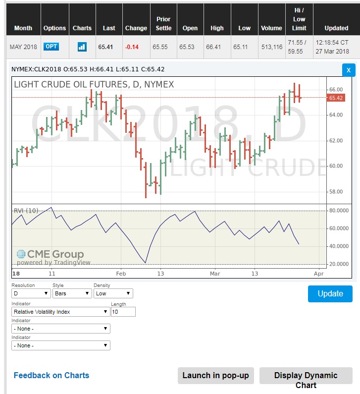
There are many other volatility measures that each give some signals and information about the price movement. Some of these measures might be a bit complicated to calculate. Some of these volatility indicators are provided in the NYMEX chart data, such as the Relative Volatility Index [7] (RVI). Relative Volatility Index gives us an indicator of the direction and magnitude of the volatility.

For example, to see the Relative Volatility Index for the WTI crude oil NYMEX futures contracts:

• Go to the NYMEX Crude Oil Futures Quotes. [8]
• Click on the Chart icon on the left side of the “Last” price.
• Make sure the chart is in the Static mode. If not, click on the “Display Static Chart”.
• From the “Indicator” list, choose the “Relative Volatility Index” and click “Update”.

The lower section of the following graph shows the Relative Volatility Index for May 2018 WTI crude oil NYMEX futures contracts. We will learn more about the RVI in lesson 9.

Correlation is a measure of the strength of the linear relationship between two quantitative variables. The equation for the correlation coefficient is:

$$r=\frac{{\displaystyle \sum \left(x_i-\overline{x}\right)\left(y_i-\overline{y}\right)}}{\sqrt{{\displaystyle \sum {\left(x_i-\overline{x}\right)}^2}}\sqrt{{\displaystyle \sum {\left(y_i-\overline{y}\right)}^2}}}$$

Correlation coefficient takes a value between -1 and 1. As you can see in the following video, a correlation coefficient of 1 indicates a strong positive linear relationship between two variables and a correlation coefficient of -1 shows a strong negative linear relationship. And if two variables are not related or not linearly related, the correlation coefficient can take a value close to zero.

Strength of linear association

As we learned in a previous lesson, a high correlation between spot and futures market prices makes the hedging efficient. Note that in the case of backwardation, the correlation between spot and futures would be lower.

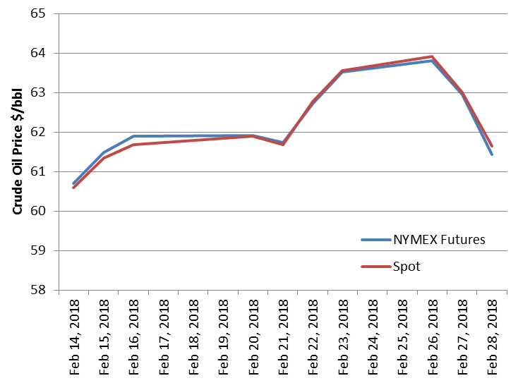
Example:

The following chart shows the last 10 prices of February 2018 crude oil spot and futures from EIA.

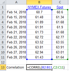
Date	NYMEX Futures [9]$/bbl	Spot [10]$/bbl
Feb 14, 2018	60.7	60.6
Feb 15, 2018	61.48	61.34
Feb 16, 2018	61.89	61.68
Feb 20, 2018	61.91	61.9
Feb 21, 2018	61.73	61.68
Feb 22, 2018	62.72	62.77
Feb 23, 2018	63.52	63.55
Feb 26, 2018	63.81	63.91
Feb 27, 2018	62.94	63.01
Feb 28, 2018	61.43	61.64

The following chart displayed the data and, as you can see, they are closely related.

As the following graph shows, we can use the Excel function CORREL() to calculate the correlation between spot and futures for these price data as 0.994, which shows a strong relationship between them.

Note that cross hedging is using futures contracts (for commodity A) in order to hedge the price risk for the commodities (commodity B) that don’t have futures contract market. And cross hedging is possible when the futures prices of commodity A are highly correlated with spot prices of commodity B.

Note that we can calculate the correlation the returns in a similar way to what we did to calculate the volatility (calculating the standard deviation for the returns).

Price Analysis

• Go to the EIA website (Spot Prices) [10] and find WTI - Cushing, Oklahoma daily spot price data.
• Go to the EIA website (NYMEX Futures Prices) [9]and find WTI - Cushing, NYMEX daily Futures Prices (Contract 1).
• Extract the last three full month daily prices for both spot and NYMEX.
• Separate each month: So, there will be three full sets of data for each, NYMEX and spot prices.
• Clean the data: make sure dates are matching.
  • In case of missing data (not the weekends), use interpolation to set the value for the missing price data.
• Draw a graph for each month and include both series (futures and spot) in the graph. There will be total of three graphs.
  • For example, include the January spot and futures in one graph.
• Calculate the correlation between spot and futures for each month.
• Calculate the 10-period moving standard deviation for spot and futures for each month.
• Calculate the 10-period volatility for spot and futures for each month's data.
• Compare the volatility in the spot market with futures market.
• • Which market is more volatile?
  • Is it consistent with what we learnt in lesson 3 and 4 about these two markets?
• Comment on the correlations
  • Which months have the lowest and highest correlations between two markets?
  • In which month hedging will be more efficient?
  • In which month hedging will be less efficient?

Note: you can use Excel or any other spreadsheet software for this assignment. Please submit the spreadsheet (Excel) file.

Grading Criteria

This activity is worth up to 20 points on the EBF 301 grading scale.

• Cleaning and organizing the data (3 points)
• Three graphs (3 points) 
• Correlation (3 points) 
• 10-period moving standard deviation for each month (3 points) 
• 10-period volatility for each month data (3 points)
• Comparing the volatilities (2 points)
• Commenting on the correlations (3 points)

---

Fundamental Factors

The Fundamental Factors activity is due as usual this week, at 11:59 pm on Sunday, and is worth 30 points on the EBF 301 grading scale. Please refer to the Fundamental Factors Instructions [11] for additional information and grading rubric.

---

Quiz

Return to Canvas to complete the L8 Quiz.

Key Learning Points: Lesson 8

1. Variation of a parameter such as price data is an important factor in risk management. 
2. A commodity with high price variation is considered a high risk investment.
3. Volatility is a term for measuring the dispersion and variation.
4. Standard deviation can be used as a measure of volatility.
5. The moving standard deviation is the standard deviation calculated for a moving window of data.
6. One measure for calculating volatility is the moving (rolling) standard deviation for the changes of price (return).
7. Price change can be calculated using an arithmetic method or using the natural log method (return).
8. Exponentially weighted volatility uses a decay factor, λ, to apply higher weights to the more recent data.
9. Relative Volatility Index is another measure of volatility.
10. Correlation is a measure of the strength of the linear relationship between two quantitative variables.
11. A strong correlation between spot and futures market prices makes the hedging efficient.

Over the past few weeks, you have been researching various Fundamental Factors that can be used to aid in making trading decisions. In the next two lessons, we will explore quantitative methods and price analysis. The other type of information, used by "day traders," is Technical Analysis. In the next lesson, we will get an elementary overview of Technical Analysis.

Reminder - Complete all of the lesson tasks!

You have reached the end of this lesson. Double-check the list of requirements on the first page of this lesson to make sure you have completed all of the activities listed there before beginning the next lesson.