Lesson 4: Mutually Exclusive Project Analysis
Introduction
Overview
Mutually exclusive projects: making an analysis of several alternatives from which only one can be selected, such as selecting the best way to provide service or to improve an existing operation or the best way to develop a new process, product, mining operation, or oil/gas reserve.
Non-mutually exclusive projects: analyzing several alternatives from which more than one can be selected depending on capital or budget restrictions, such as ranking research, development, and exploration projects to determine the best projects to fund with available dollars.
This lesson focuses on the analysis of mutually exclusive alternatives. Valid discounted cash flow criteria such as rate of return, net present value, and benefit-cost ratio are applied in very different ways in proper analysis of mutually exclusive and non-mutually exclusive alternative investments.
Learning Objectives
At the successful completion of this lesson, students should be able to:
- understand how to use rate of return and NPV analysis to evaluate mutually exclusive projects and non-mutually exclusive projects;
- understand how to conduct Incremental Analysis; and
- understand how variable minimum rate of return with time can affect the project.
What is due for Lesson 4?
This lesson will take us one week to complete. Please refer to the Course Syllabus for specific time frames and due dates. Specific directions for the assignment below can be found within this lesson.
| Reading | Read Chapter 4 of the textbook. |
|---|---|
| Assignment | Homework 4. |
Questions?
If you have any questions, please post them to our discussion forum, located under the Modules tab in Canvas. I will check that discussion forum daily to respond. While you are there, feel free to post your own responses if you, too, are able to help out a classmate.
Using Rate of Return, Net Value and Ratios for Mutually Exclusive Projects
Economic analysis of projects can be divided into two categories:
1) Mutually Exclusive
2) Non-Mutually Exclusive
Mutually Exclusive type analysis is where the investor faces different investment alternatives, but only one project can be chosen for investment. Selecting one project excludes other projects from investment.
Non-Mutually Exclusive assessments are where the investor faces different alternatives, but more than one project can be selected regarding capital or budget constraint.
Rate of Return Analysis for Mutually Exclusive Alternatives
Example 4-1: Assume an investor has two alternatives, project A and project B, and other opportunities exist to invest at 15% ROR. The total money that investor has is 400,000 dollars.
Project A: Includes investment of 40,000 dollars at present time which yields an income of 40,000 dollars for 5 years and the salvage value at the end of the fifth year is 40,000 dollars.
| C=$40,000 | I=$40,000 | I=$40,000 | I=$40,000 | I=$40,000 | I=$40,000 | L=$40,000 | |
| A) |
|
||||||
| 0 | 1 | 2 | 3 | 4 | 5 | ||
Project B: Includes investment of 400,000 dollars at the present time which yields the income of 200,000 dollars for 5 years and the salvage value at the end of the fifth year is 400,000 dollars.
| C=$$400,000 | I=$200,000 | I=$200,000 | I=$200,000 | I=$200,000 | I=$200,000 | L=$400,000 | |
| B) |
|
||||||
| 0 | 1 | 2 | 3 | 4 | 5 | ||
C: Cost, I:Income, L:Salvage
ROR analysis for project A:
With trial and error or using the IRR function in Excel, we can calculate . So project A is satisfactory.
ROR analysis for project B:
With trial and error or using the IRR function in Excel, we can calculate . So project B is also satisfactory.
Many people think because project A has a higher ROR, project A has to be selected over project B. But remember, we assumed 400,000 dollars is available for the investment, and the investor can only choose one of the projects. Project A takes just 10 percent of the money and gives 100% ROR, while project B takes the entire 400,000 dollars and gives 50% ROR. If the investor chooses project A and spends 40,000 dollars on this project, the rest of the money can only be invested with a 15% ROR. So, we need one more step that is called incremental analysis to be able to compare two projects and determine which project is better. The incremental analysis helps up to find a common base to compare two projects. To do so, incremental analysis breaks project B into two projects: one is similar to project A and the other is an incremental project.
Project B is equivalent to
Please note that the investing in Project B (requires $400,000) is equivalent to investing
Choosing project A with 100% ROR + investing the rest of money with 15%
Or
Choosing project B, which is equivalent to an investment in project A with 100% ROR+ investment in the incremental project (B-A)
The incremental analysis has to be done for the bigger project minus the smaller one as:
| C=$360,000 | I=$160,000 | I=$160,000 | I=$160,000 | I=$160,000 | I=$160,000 | L=$360,000 | ||
| B-A |
|
|||||||
| 0 | 1 | 2 | 3 | 4 | 5 | |||
This investment gives 44.4 % return.
So, incremental analysis shows that investment in project B is equivalent to investing in A (which gives 100% ROR) plus investing in project B-A (which gives 44%).
Thus, the second alternative, project B, is more desirable.
1) the rate of return on total individual project investment must be greater than or equal to the minimum rate of return, i*.
2) the ROR on incremental investment compared to the last satisfactory level of investment must be greater than or equal to the minimum ROR, i*.
The largest level of investment that satisfies both criteria is the economic choice.
Therefore, in mutually exclusive projects, a smaller ROR on a bigger investment often is economically better than a big ROR on a smaller investment. Therefore, it is often preferable to invest a large amount of money at a moderate rate of return rather than a small amount at a large return with the remainder having to be invested elsewhere at a specified minimum rate of return.
Please watch the following video (11:56): Mutually exclusive projects (Rate of return analysis).
PRESENTER: In this video, I'm going to explain how we can evaluate mutually exclusive projects. If you are given more than one investment project to evaluate, then you're facing two types of investments. It is either a non-mutually exclusive or mutually exclusive kind of problem. In a non-mutually exclusive assessment, you can choose more than one project. In this case, you will rank the project based on the parameter that you learn, such as the MPV rate of return and so on, and choose the projects from the best to worse.
But here, in this lesson, we are going to work on mutually exclusive evaluations. In this case, in mutually exclusive assessments, we have a budget constraint, so we can only choose one project. So we need to evaluate all projects and select the best project that is economically satisfactory.
Let's work on an example. Assume an investor has two alternatives, project A and project B, and other opportunities exist to invest at a 15% rate of return. And this 15% rate of return means we can make at least 15% on the $400,000 if we invest somewhere else. The $400,000 that isn't required for investment in project A or project B.
So it means each of these two projects, project A and project B are economically satisfactory only if each of them gives a return of higher than 15%. If they don't, they are not economically satisfactory, and we can invest in the other project with the 15% rate of return. So our minimum rate of return or minimum discount rate is 15%. This is the rate that we have to compare our individual assessment with.
So let's calculate the rate of return for these projects. So in order to evaluate and find-- in order to evaluate and find the best project, first, we have to evaluate each project individually. Then we compare the projects that are economically satisfactory and choose the best one. So let's calculate the rate of return for project A and project B.
First, we write the equation for the rate of return-- the present value of cost equals the present value of income plus salvage. And we calculate rate of return for project A as 53%, which is higher than 15% minimum rate of return. So it tells us that project A is economically satisfactory.
Now let's calculate the rate of return for project B. We write the equation. So we can see the rate of return for project B is 50%, which is higher than 15% of the minimum rate of return. So project B is also economically satisfactory. So because project A has a higher rate of return with the same amount of investment, we can conclude that project A has to be selected for the investment.
Now let's work on a slightly different example. Let's assume that the investor has $400,000 available for the investment. The investor has two alternatives, project A and project B, and other opportunities exist to invest at 15% rate of return. As you can see here, project A requires $40,000, but we have $400,000 money available for the investment. Again, first, we have to evaluate the projects individually, and then we compare the projects that are economically satisfactory and choose the best one.
So for project A, we write the equation to calculate the rate of return. And we calculate rate of return as 100%, which is higher than the 15% of minimum rate of return, so project A is economically satisfactory. Then we calculate the rate of return for project B. We write the equation, and we calculate the rate of return, which is 50%. 50% is higher than the minimum rate of return of 15%, so project B is also economically satisfactory.
So the results show that project A has a higher rate of return than project B. Let's see if project A is the best project for the investment or not. Using the rate of return for mutually exclusive projects can be confusing, and it doesn't necessarily give us the best economic choice. Remember, we had $400,000 available to investment, but project A is using only $40,000 of that $400,000. Project A is giving us a 100% return on $40,000, but project B is giving us a 50% return on the total $400,000.
This means if you invest in project A, then you will have an extra $360,000 that you can only invest in the other project with 15% return because project A requires only $40,000, but we have $400,000 available for the investment. So the rest of the money, that $360,000, can't be put in any other project other than the project that gives the minimum rate of return of 15%.
So there are two alternatives for the investment of $400,000. The first one is investing the $40,000 in project A with the rate of return of 100%, plus investing the rest of $360,000 with the rate of return of 15%. Or the second alternative is investing the entire $400,000 in project B with the rate of return of 50%. So we need to find a base to compare these two projects together.
In this case, we need incremental analysis, which breaks the project B into two projects. One is similar to project A and the other is an incremental project or B minus A. So project B is equivalent to project A-plus project B minus A because project A requires much less investment, and the rest of the money can only be invested in the minimum rate of return of 15%.
In order to evaluate the project B minus A, we need to deduct the project A cash inflow from the project B cash flow. So here, each year, each column, cash flow equals the project B minus project A. We write the rate of return equation for incremental cash flow-- the present value of cost equals the present value of income plus the present value of salvage. The present value of cost equals $360,000, which is the difference between project A and project B investment, and the $160,000, which is the difference between annual income for project A and Project B, and the $360,000 in year five, which is the difference between salvage values.
And we can use the Excel IRR function to calculate the rate of return. So incremental cash flow has the rate of return of 44.4%, and it is economically satisfactory. It means project B that has a rate of return of 50% is equivalent to project A with a 100% rate of return plus an incremental project with 44%.
So we have two alternatives. The first one is investing $40,000 at the rate of return of 100% plus investing $360,000 at the minimum rate of return of 15% or investing the entire $400,000 in project B, which is equivalent for investing in a project, similar to project A, with $40,000 of investment and the rate of return of 100% plus investing in the incremental project, which needs $360,000.
And the rate of return would be 44.4%. And we can conclude that project B is more desirable investment although project B has a lower rate of return. But because it uses the entire $400,000, it is a better project to invest.
When using the rate of return analysis for the evaluation of mutually exclusive projects, we need to keep two things in our mind. First, the rate of return for each individual project has to be higher than the minimum rate of return. And also, the rate of return on the incremental investment has to also be higher than the minimum rate of return.
And the largest level of investment that satisfies both criteria is the economic choice, So it is often more desirable to invest a large amount of money at a moderate rate of return rather than investing a small amount of money at a large rate of return because we need to invest the rest of the money at a minimum rate of return.
Net Present Value (NPV) Analysis of Mutually Exclusive Alternatives “A” and “B”
Considering a discount rate of 15% (minimum rate of return), the NPV for project A and B can be calculated as:
Since the NPV for project A and B is positive at the 15% discount rate (minimum rate of return on investment), then we can conclude that both projects are economically satisfactory. But NPV for project B is higher than A, which means B is a better choice to invest.
Incremental NPV Analysis
We can also calculate the incremental NPV as:
Note that incremental NPV is exactly equal to the difference between NPVA and NPVB:
The incremental at a 15% discount rate is positive, which means the incremental investment is economically satisfactory.
Remember the two decision alternatives that the investor faces:
1) Choosing project A + investing the rest of money with 15%
2) Choosing project B, which is equivalent to an investment in project A + investment in the incremental project (B-A)
The NPV for the first decision is:
1) NPVA + NPV (of investing the remainder of the available money somewhere else with a 15% rate of return)
If an investment return of 15%, then the NPV at a discount rate of 15% for that investment cash flow equals zero. So:
1)
The NPV for the second decision is:
2)
Therefore, it can be concluded that investment in project B is a better decision.
In summary, for net present value analysis of mutually exclusive choices, two requirements need to be tested: 1) the net value on total individual project investment must be positive, and 2) the incremental net value obtained in comparing the total investment net value to the net value of the last smaller satisfactory investment level must be positive. The largest level of investment that satisfies both criteria is the economic choice. Or simply, the project with the largest positive net present value is the best choice.
Note: You can use Microsoft Excel and the NPV function in order to calculate Net Present Value as explained in Example 3-6 in Lesson 3.
Please watch the following video (3:37): Mutually exclusive alternatives
PRESENTER: Another method to evaluate the mutually exclusive projects is the NPV analysis. So let's work on the same example using the NPV analysis.
Assume an investor has two alternatives, Project A and Project B, and the total money that the investor or has is $400,000, and the minimum rate of return is going to be 15%
First, we have to evaluate each project individually, and then we compared to projects that are economically satisfactory and choose the best one. So first, we have to calculate the NPV for Project A. We used the minimum rate of return of 15% as a discount rate for calculating the NPV. And because the NPV of Project A at a discount rate of 15% is positive, so we can conclude that Project A is economically satisfactory.
And then we calculate the NPV for Project B. NPV of Project B at a minimum rate of return of 15% is also positive, so Project B is also economically satisfactory.
So Project A and Project B, both have positive NPVs, so both of them are economically satisfactory. And because Project B has a higher NPV, we can conclude that Project B is a better project to invest in. This is a very good thing about NPV, that if a project has a higher NPV, we can directly conclude that that project is a better choice to invest.
We can also calculate the NPV for the incremental cash flow, which we can see here, it is positive, and we can conclude Project B is better than Project A.
But there is a good property for NPV operator is NPV of the incremental analysis, NPV of B minus A equals NPV of Project B minus NPV of Project A. So that's the reason that if we calculate the NPV of Project B higher than Project A, we can conclude that Project B is a better project to invest, because the difference shows us the increment, directly shows us the NPV of the incremental cash flow.
So again, we have two alternatives here, choosing Project A and investing the rest of the money at the 15% minimum rate of return, or choosing Project B, which is equivalent to investing in Project A plus investing in the incremental Project B minus A.
And because incremental NPV at a 15% discount rate is positive, it means that incremental investment is economically satisfactory, which means that a second alternative, or Project B, is a more desirable scenario.
Ratio Analysis of Mutually Exclusive Projects A and B
Present value ratio (PVR) also can be applied to analyze two mutually exclusive projects, A and B:
Positive PVR for project A and B indicates that both projects are economically satisfactory. But higher PVR for project A doesn’t necessarily mean project A is better than B for investment and PVR needs to be calculated for an incremental project as well.
Accepting the incremental investment indicated accepting project B over A, even though the total investment ratio on B is less than A. Just as with ROR analysis, the mutually exclusive alternative with bigger ROR, PVR is not necessarily a better mutually exclusive investment. Incremental analysis along with total individual project investment analysis is the key to a correct analysis of mutually exclusive choices.
Mutually Exclusive Projects with Unequal Life
If mutually exclusive projects that are being analyzed don’t have the same lifetimes (for example, one investment has a length of 8 years and the other alternative example has the length of 12 years), we have to be careful using the parameters that we have learned so far.
NPV analysis
We can continue the NPV analysis without any problem for mutually exclusive projects with different lifetimes. This is because NPV analysis considers a common point in time for all projects, which is the present time.
It is also important to know that for NPV analysis, different discount rates may cause different results and may change the ranking of the projects. Thus, the selected discount rate for such should be representative of the opportunity cost of capital for consistent economic decision-making.
ROR analysis
For ROR analysis (and other analysis, such as future value, that require a specific point on the timeline) of mutually exclusive projects with different lifetimes, we need to find a common lifetime and analyze the alternatives based on that. This common lifetime is usually the longest lifetime between alternatives.
For ROR analysis, treat all projects as having an equal life that is equal to the longest life project with net revenues and costs of zero in the later years of shorter life projects.
Example 4-2:
Consider the following two mutually exclusive projects:
Assume a minimum rate of return of 8%
Project A
| C=1000 | I=250 | I=250 | I=250 | I=250 | I=250 | I=250 | I=250 |
|
|
|||||||
| 0 | 1 | 2 | 3 | 4 | 5 | 6 | 7 |
Project B
| C=2000 | C=3000 | I=1000 | I=1000 | I=1000 | I=1000 | I=1000 | I=1000 | I=1000 | I=1000 | I=1000 |
|
|
||||||||||
| 0 | 1 | 2 | 3 | 4 | 5 | 6 | 7 | 8 | 9 | 10 |
First, we need to evaluate each project individually and see if both are economically satisfactory.
Project A evaluation:
For project A: ROR> i*=8%, NPV is positive, B/C is higher than 1, and PVR is positive. So, project A is economically satisfactory.
Project B evaluation:
For project B: ROR> i*=8%, NPV is positive, B/C is higher than 1, and PVR is positive. So, project B is also economically satisfactory.
Please note that project A has a lifetime of seven years, while project B’s lifetime is 10 years. In this case, we chose the project with the longest lifetime (here, project B) as the base case and put zero for the years that project A doesn’t have any payment. Then we deduct the cash flow of project A from the cash flow of project B as incremental cash flow:
| -1000 | -3250 | 750 | 750 | 750 | 750 | 750 | 750 | 1000 | 1000 | 1000 |
|
|
||||||||||
| 0 | 1 | 2 | 3 | 4 | 5 | 6 | 7 | 8 | 9 | 10 |
Since the incremental project (B-A) is economically satisfactory, we can conclude that project B is better than project A.
Note that
Example 4-3:
Consider this situation that a manager faces. There are three alternatives:
- investing in development plan A, as shown in the following cash flow;
- investing in development plan B, as shown in the following cash flow;
- selling the property for $150 in cash. Apply the ROR, NPV, and PVR analysis to find the best economic alternative assuming a minimum rate of return of 15%, and then repeat the assessment for a minimum rate of return of 20%.
| Year | 0 | 1 | 2 | 3 | 4 | 5 | 6 | 7 | 8 | 9 | 10 |
|---|---|---|---|---|---|---|---|---|---|---|---|
| A | -200 | -350 | 100 | 100 | 150 | 150 | 150 | 150 | 150 | -- | -- |
| B | -300 | -400 | 200 | 200 | 200 | 200 | 200 | 200 | 200 | 200 | 200 |
| Sell | 150 | -- | -- | -- | -- | -- | -- | -- | -- | -- | -- |
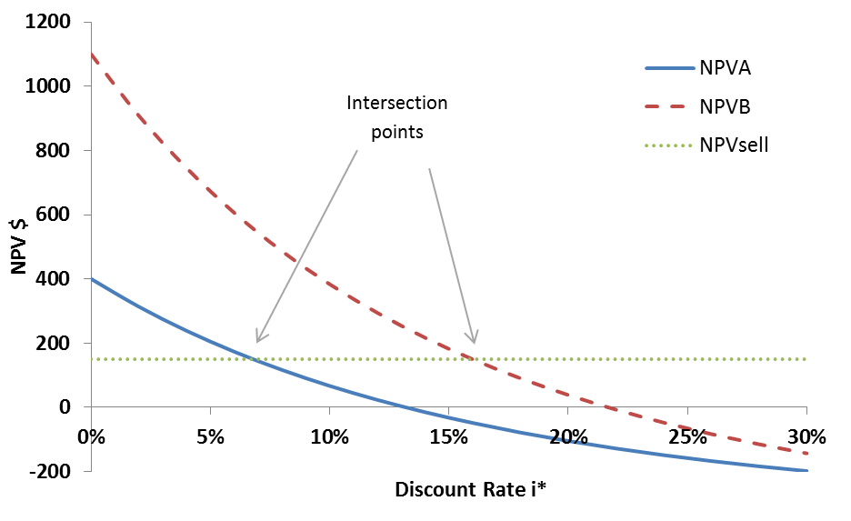
Figure 4-1: cash flow for three alternatives: 1) Development plan A, 2) Development plan B, 3) Sell the property
RORA = 13.2% ROR is less than minimum rate of return of 15%, so the project is not economically satisfactory
. NPV is negative, so the project is not economically satisfactory
. PVR is negative, so the project is not economically satisfactory.
RORB=21.65% ROR is higher than the minimum rate of return of 15%, so the project is economically satisfactory
. NPV is positive, so the project is economically satisfactory
. PVR is positive, so the project is economically satisfactory.
ROR, NPV, and PVR analysis indicate that development plan B is better than investing money at a minimum rate of return of 15%.
The NPV, ROR, and PVR for selling the property:
RORsell = +∞ higher than the minimum rate of return of 15%, so the project is economically satisfactory
NPVsell = +150 is positive, so the project is economically satisfactory
PVRsell = +∞ is positive, so the project is economically satisfactory
Since NPVB is higher than NPVsell, the above analyses show that development plan B is the best economic choice among the three alternatives.
In order to compare development plan B and selling the property, we can also apply the incremental analysis as:
| Year | 0 | 1 | 2 | 3 | 4 | 5 | 6 | 7 | 8 | 9 | 10 |
|---|---|---|---|---|---|---|---|---|---|---|---|
| B-sell | -450 | -400 | 200 | 200 | 200 | 200 | 200 | 200 | 200 | 200 | 200 |
which is greater than 15%, so project B is economically satisfactory.
is positive, so it is economically satisfactory.
0.04 is positive, so it is economically satisfactory.
As previously explained, the incremental analysis will always lead to selecting the alternative with the largest individual NPV. Therefore, development plan B is the best economic choice. However, note that project B does not have the highest ROR or PVR.
Assuming the minimum rate of return of 20%
It is negative, so the project is not economically satisfactory.
. NPV is positive, so the project is economically satisfactory
NPVsell= +150 is positive, so the project is economically satisfactory.
Therefore, at a minimum rate of return of 20%, selling the property is the best economic choice.
As calculations show, results are sensitive to discount rates (minimum rate of return)
Mutually exclusive projects with different starting dates
Example 4-4:
Consider two alternatives: development plan B, and selling the property. But assume that development plan B will start in the second year. Which project is the best economic choice at a minimum rate of return of 15%?
Cash flow for these alternatives:
| Year | 0 | 1 | 2 | 3 | 4 | -- | 12 |
|---|---|---|---|---|---|---|---|
| B | -- | -- | -300 | -400 | 200 | 200 | 200 |
| Sell | 150 | -- | -- | -- | -- | -- | -- |
In this case, NPV indicates that selling the property is the best economic choice. NPV is positive, so it is economically satisfactory.
NPVsell=150 is positive, so it is economically satisfactory.
Incremental analysis can also be done as:
| Year | 0 | 1 | 2 | 3 | 4 | -- | 12 |
|---|---|---|---|---|---|---|---|
| B-sell | -150 | -- | -300 | -400 | 200 | 200 | 200 |
RORB-sell = 14.57% which is lower than 15% minimum rate of return
which is negative, so it is not economically satisfactory.
Thus, choosing development plan B overselling the property is not economically acceptable.
Changing the Minimum Rate of Return with Time
So far, we have assumed that minimum rate of return is fixed over the life of the project. But there are situations where other opportunities for investment (that determine the minimum rate of return) can make different rate of returns in different time. Thus, minimum rate of return can change over time. For example, other opportunities for investment of capital can give i*=12% now; and three years from now, we might expect a project that has a return on investment of i*=15%.
For analyses with minimum rate of return that change with time, NPV and PVR are recommended as the best methods. ROR is not a reliable approach for such analyses.
Example 4-5:
Cash flows for two mutually exclusive investment projects A and B are given as:
| C=$40 | I=$20 | I=$20 | I=$20 | I=$20 | I=$20 | L=$40 | |
| A) |
|
||||||
| 0 | 1 | 2 | 3 | ... | 10 | ||
| C=$50 | I=$25 | I=$25 | I=$25 | I=$25 | I=$25 | L=$50 | |
| B) |
|
||||||
| 0 | 1 | 2 | 3 | ... | 10 | ||
C: Cost, I:Income, L:Salvage
Analyze these alternatives, assuming the minimum rate of return for the first and second years is 25% and for third to tenth year it is 15%.
Results indicate that project B is a better economic investment.
Note:
After year 2, minimum rate of return changes from 25% to 15%. In order to calculate the NPV of the cash flow, we have to separate the payments that happened at and before year 2 from payments that occurred after year 2.
Payments at year 2 and before that are not going to be affected by the change:
PV of payments from year 0 to year 2:
Project A: Present value of year 0 to year 2 payments
Project B: Present value of year 0 to year 2 payments
But payments after year 2 will be affected by the change.
To calculate the NPV of those payments and apply the change in i, first, we need to discount all the payments occurred after year 2 to this year (we set the year 2 as the base year) by i* = 15% and we calculate value of all payments at year 2:
Project A: Value of year 3 to year 10 payments at year 2
Project B: Value of year 3 to year 10 payments at year 2
Second, we discount the year 2 values for 2 years by i* = 25%to get the present value (value at year 0) of the payments:
Project A: Present Value of year 3 to year 10 payments
Project B: Present Value of year 3 to year 10 payments
In the end, we add all the values together:
Another Method:
You can also treat each payment separately. This method is especially helpful when payments are not equal or when you are using spreadsheet to calculate the NPV.
We separate the payments that happened at and before year 2 from payments after year 2. Payments at and before year 2 will be discounted just by 25%:
PV of payments from year 0 to year 2:
Project A: PV year 0 to year 2
Project B: PV year 0 to year 2
For payments after year 2, first we calculate their value at year 2:
Project A: Value of year 3 to year 10 payments at year 2
Project B: Value of year 3 to year 10 payments at year 2
Second step, we discount the year 2 values for 2 years by i* = 25% to get the present value (value at year 0) of the payments:
Project A: Present Value of year 3 to year 10 payments
Project B: Present Value of year 3 to year 10 payments
In the end we add all the values together:
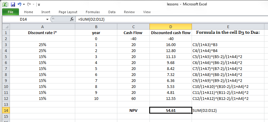
Microsoft Excel or Spreadsheet
If you are using Microsoft Excel or another spreadsheet to calculate the Net Present Value for the cash flow that has different discount rates over the life of project, be careful! You can not use the NPV function. However, you can calculate the Net Present Value by making a summation over calculated discounted cash flow. Figure 4-3 displays how Net Present Value for Project A cash flow with a changing minimum rate of return can be calculated. Note the formula in the cell D3 to D12.
PRESENTER: So far, we assume the minimum rate of return in our analysis is fixed over the lifetime of the project. And it's not changing over time. But there are situations that we might have other opportunities for investment later on in the following years. So our minimum rate of return might change.
And it means that the discount rate, the minimum discount rate that we are using in our analysis will change too. In this video, I'm going to explain how we can evaluate the mutually exclusive projects or, in general, any other project if the minimum rate of return, if the discount rate changes over the lifetime of a project. So if the minimum rate of return changes with the time, the NPV and PVR present value ratio are recommended as the best methods. And rate of return is not a reliable approach for the project evaluation.
Let's work on this example. We have the cash flow for Project A and Project B that are mutually exclusive. And we assume the minimum rate of return for the first and second year is 25%. And the minimum rate of return changes to 15% from year 3 to year 10. So the first thing that we have to do is to separate the payments before the change and after the change.
So here, minimum rate of return changes after year 2. So I draw this red vertical line here to separate the payments before this year and payments that are after year 2. Return of present value of 40. Present value of these 20 payments at year 1 and 2. So present value of 40 is $40. And it is negative because it's a cost, it's an investment, and it's happening at present time. So there is no discounting needed here.
But two payments. We have two payments of $20 at year 1 and year 2. We discount them on 25%. And there are two of them. And then we need to calculate the present value of payments that are happening after year 2.
These payments are going to be affected by the change in the minimum rate of return. So first, we need to calculate the present value of these payments at 15% rate of return through the year 2 and then after discount at present value for 2 years with 25% of discount rate. So here, we have 8 payments of $20.
So we discount them 20 year 2 by the 15%. And then after, we discount that by 25% for 2 years. That is going to give us the present value here. And for the salvage value, it's the same. We discount the salvage value for 8 years at 15% and then we discount that after 2 years by 25%.
So we use this method to calculate the present value, net present value, NPV, for two mutually exclusive projects. And as we can see here, Project B has higher net present value. So I'm going to show you how we can calculate this in Excel using the other method, calculating the present value of each payment, and then add them back together. So I have the cash flow of Project A here, cash flow of Project B, and I wrote the minimum rate of return here for each year.
So as we can see here, we have 25% for year 1 and 2. And we have 15% from year 3 to year 10. So cash flow of Project A, cash flow of Project B. And for the last year, I added the salvage to the annual payment of the last year. So Project A, I'm going to calculate the present value of each payment in this cell.
So present value of these $40 of investment is going to be the same as $40. It doesn't need to be discounted because it is happening at the year 0. So present value of the $20. So I write equal sign at $20 divided by 1 plus interest rate, power, the year. So this is not going to be affected by change in the minimum rate of return.
So these 2 years are the same, so I just apply this equation to for the year 2. But for the year 3, how do we calculate the present value of this $20 that is happening at year 3? So it is going to be affected by two interest rates. 20 divided by open parentheses, 1 plus 15% power. So this needs to be discounted for 1 year because minimum rate of return changes at year 2. And this payment is 1 year away from year 2.
So I write year 1. And again, I have to divide that. I have to discount that by 2 years because this is going to give me the present value of this $20 here. And then I need to discount that at the rate of 25% for 2 more years. So 1 plus 25% power 2. And this is the same for the rest. So in order to apply these to the other cells, I will just write for this.
So read the year from here and minus 2, which is the year that the minimum rate of return changes. And I apply this to the other cash flow. And the same for Project B. Investment at present time as the same for year 1. It equals 1 plus 25% power the year.
For year 1 and year 2, there are similar. For year 3, this is 25 divided by open parentheses 1 plus 15% interest rate power year minus 2. And again, this divided by 1 plus 25% power 2.
And I apply this to the end. So these two should give me the present value. And I calculate the NPV for Project A, NPV for Project B. NPV for Project A equals the summation of all these present values. And the same for B.
Summary and Final Tasks
Summary
1. Mutually Exclusive Alternative Analysis
The Rate of Return or Growth Rate of Return: With either regular ROR or Growth ROR analysis of mutually exclusive alternatives, you must evaluate both total investment ROR and incremental investment ROR, selecting the largest investment for which both are satisfactory. Use a common evaluation life for Growth ROR analysis of unequal life alternatives, normally the life of the longest life alternative assuming net revenues and costs are zero in the later years of shorter life alternatives.
Net Value Analysis: With NPV analysis, you want the mutually exclusive alternative with the largest net value – because this is the alternative with the largest investment that has both a positive total investment net value and a positive incremental net value compared to the last satisfactory smaller investment.
2. Non-Mutually Exclusive Alternatives
The Rate of Return or Growth Rate of Return: Regular ROR analysis cannot be used to consistently rank non-mutually-exclusive alternatives. Use Growth ROR, and rank the alternatives in the order of decreasing Growth ROR. This will maximize profit from available investment capital. Use a common evaluation life for Growth ROR analysis for unequal life alternatives, normally the life of the longest alternative.
Net Value Analysis: With NPV analysis of non-mutually exclusive projects, select the group of projects that will maximize cumulative net value for the dollars available to invest. This does not necessarily involve selecting the project with the largest net value on individual project investment.
Reminder - Complete all of the Lesson 4 tasks!
You have reached the end of Lesson 4! Double-check the to-do list on the Lesson 4 Overview page [1] to make sure you have completed all of the activities listed there before you begin Lesson 5.