Lesson 6: Uncertainty and Risk Analysis
Introduction
Overview
In this era of advancing technology, successful managers need to make investment decisions that determine the future success of their companies by drawing systematically on the specialized knowledge, accumulated information, experience, and skills of many people. In previous lessons, the investment analyses were all considered to be made under "no-risk" conditions. In this lesson, we add in the uncertainties when evaluating an energy/mining project. The objective of investment decisions is to invest available capital where we have the highest probability of generating the maximum possible future profit. The use of quantitative approaches to incorporate risk and uncertainty into analysis results may help us be more successful in achieving this objective over the long run.
Learning Objectives
At the successful completion of this lesson, students should:
- understand how to conduct sensitivity analysis to analyze the effects of uncertainty;
- be able to conduct expected value analysis; and
- understand the risk due to natural disasters.
What is due for Lesson 6?
This lesson will take us one week to complete. Please refer to the Course Syllabus for specific time frames and due dates. Specific directions for the assignment below can be found within this lesson.
| Reading | Read Chapter 6 of the textbook. |
|---|---|
| Assignment | Homework and Quiz 6. |
Questions?
If you have any questions, please post them to our discussion forum, located under the Modules tab in Canvas. I will check that discussion forum daily to respond. While you are there, feel free to post your own responses if you, too, are able to help out a classmate.
Risk Analysis
So far, in previous lessons, effect of risk and uncertainty haven’t been considered in our economic evaluations and the analyses were assumed to be of no-risk condition. In this case, the probability of success and achieving anticipated results is assumed to be 100%, but in reality, some degree of uncertainty is involved and this probability is much lower. The economic analyses that don’t include risk and uncertainty are based on “best guess,” and the results aren’t highly accurate and reliable. For example, if a study shows 20% and 25% ROR for project A and B, the manager would probably choose project B over A. But what if the probability of success is 90% for project A and 40% for project B? This example shows how important it is to consider the effect of risk and uncertainty as a component in economic evaluations.
Quantitative methods, along with informal analysis, are used for decision making under risk and uncertainty. Quantitative methods aim to provide the best possible set of information to decision-makers so that they may apply their experience, intuition, and judgment to achieve the final decision; the decision that leads to maximum possible future profit with the highest probability. There are several different approaches that can be used to quantitatively incorporate risk and uncertainty into analyses. These include sensitivity analysis or probabilistic sensitivity analysis to account for uncertainty associated with possible variation in project parameters, and expected value or expected net present value or rate of return analysis to account for risk associated with a finite probability of failure. The use of sensitivity analysis is advocated for most economic analyses and the use of expected value analysis is advisable if a finite probability of project failure exists. Sensitivity analysis is a means of evaluating the effects of uncertainty on investment by determining how investment profitability varies as the parameters are varied that effect economic evaluation results.
Sensitivity analysis can show how results change if the input parameter changes. If we change one input parameter (such as initial investment) and the result (such as NPV of the project) varies significantly in a wide range, then we say the result is sensitive to the specified input parameter. Here, we aim to find the most sensitive variables. The input parameter investigated for sensitivity analysis usually includes initial investment, selling price, operating cost, project life, and salvage value. If probabilities of occurrence are associated with various levels of each investment parameter, sensitivity analysis becomes probabilistic sensitivity analysis.
It may now be evident to you that the term “uncertainty” as used in this lesson refers to possible variation in parameters that effect investment evaluation. “Risk” refers to the evaluation of an investment using a known mechanism that incorporates the probabilities of occurrence for success and failure and/or of different values of each investment parameter. Both uncertainty and risk influence almost all types of investment decisions, but especially investment involving research and development for any industry and exploration for minerals and oil or gas.
Please watch the following video (3:24): Risk, Uncertainty, and Sensitivity Analysis.
PRESENTER: In this video and the next videos, I will explain how to incorporate risk and uncertainty in the economic evaluation of projects for the purpose of investment. I will explain how we can apply the sensitivity analysis techniques to evaluate the project in this case. In previous lessons, in previous videos, we use fixed numbers. All the numbers that we used were deterministic at no risk condition. The probability of achieving an outcome was 100%.
But it is not the case in real life. There is always some level of uncertainty in the anticipated result, especially things that are happening in the future. For example, if an evaluation of two projects, Project A and Project B shows that Project A has a rate of return of 20% and Project B has a rate of return of 25%, assuming they have the same skill and they require the same amount of investment, what would you do as a manager?
You would choose the project with a higher rate of return. So you will choose Project B, which has a higher rate of return. But what if I tell you the probability of success in Project A is 90% and the probability of success in Project B is just 40%? What would be your decision?
Decision-makers use combinations of qualitative and quantitative methods in risk situations. In this video, we are focusing on quantitative methods. Quantitative methods are aiming to provide the best possible information for the decision-maker. And in the end, decision-makers have to use their own experience, intuition, and judgment for the final decision about maximum possible profits in the future with the highest probability.
There are several quantitative methods for incorporating risk and uncertainty. I will explain two of these methods in this video and the following videos. The first one is called sensitivity analysis or probabilistic sensitivity analysis. And the next one is going to be expected value or expected net present value.
Sensitivity analysis is a method that helps us understand the sensitivity of results to the input variables. Here, our result, our evaluation result, is a measure that shows us the profitability of the project, which it is NPV, rate of return, or any other parameter that we learned so far. In a sensitivity analysis, we want to determine how results vary if we change input variables. What would be the magnitude of change in one variable with respect to the change in other variables? Sensitivity analysis helps decision-makers to find the parameters that have the biggest impact on the results.
Italicized sections are from Stermole, F.J., Stermole, J.M. (2014) Economic Evaluation and Investment Decision Methods, 14 edition. Lakewood, Colorado: Investment Evaluations Co.
Uncertainty and Sensitivity Analysis
As explained before, in sensitivity analysis, we aim to discover the magnitude of change in one variable (here, output variables) with respect to change in other variables (here, input parameters). Then, we can rank the variables based on their sensitivity. It helps the decision-maker to understand the parameters that have the biggest impact on the project.
The following example introduces a single variable sensitivity analysis. Please note that here we assume variables are independent and have no effect on each other. For example, it is assumed that the magnitude of initial investment doesn’t affect the operating costs.
Example 6-1:
For a project, the most expected case includes an initial investment of 150,000 dollars at the present time, an annual income of 40,000 for five years (starting from the first year), and a salvage value of 80,000. Evaluate the sensitivity of the project ROR to 20% and 40% increase and decrease in initial investment, annual income, project life, and salvage value.
Before-tax cash flow of this investment can be shown as:
|
-$150,000
|
$40,000
|
$40,000 | $40,000 | $40,000 | $40,000 |
$80,000
|
|
|
||||||
|
0
|
1
|
2
|
3
|
4 |
5
|
|
The most expected ROR based on the most expected initial investment, annual income, and salvage value can be calculated as:
The most expected ROR will be 20.5%.
A) Sensitivity Analysis of initial investment
| Initial investment | Change in prediction | ROR | Percentage change in 20.5% ROR prediction |
|---|---|---|---|
| 90,000 | -40% | 43.5% | 112.7% |
| 120,000 | -20% | 29.6% | 44.8% |
| 150,000 | 0 | 20.5% | 0% |
| 180,000 | 20% | 13.8% | -32.6% |
| 210,000 | 40% | 8.6% | -57.8% |
As you can see, changes in ROR with respect to changes in initial investment are considerably high. In general, parameters that are close to time zero have a higher impact on the ROR of the project.
B) Sensitivity Analysis of project life
| Project life | Change in prediction | ROR | Percentage change in 20.5% ROR Prediction |
|---|---|---|---|
| 3 | -40% | 12.9% | -36.6% |
| 4 | -20% | 17.7% | -13.5% |
| 5 | 0 | 20.5% | 0% |
| 6 | 20% | 22.2% | 8.7% |
| 7 | 40% | 23.4% | 14.5% |
Note that changes in the project ROR become smaller as the project life gets longer.
C) Sensitivity Analysis of annual income
| Annual income | Change in prediction | ROR | Percentage change in 20.5% ROR prediction |
|---|---|---|---|
| 24,000 | -40% | 8.1% | -60.6% |
| 32,000 | -20% | 14.3% | -30.0% |
| 40,000 | 0 | 20.5% | 0% |
| 48,000 | 20% | 26.5% | 29.5% |
| 56,000 | 40% | 32.4% | 58.5% |
Changes in annual income also have a significant effect on ROR because these changes start happening close to present time.
D) Sensitivity Analysis of salvage value
| salvage value | Change in prediction | ROR | Percentage change in 20.5% ROR prediction |
|---|---|---|---|
| 48,000 | -40% | 17.0% | -17.0% |
| 64,000 | -20% | 18.8% | -8.2% |
| 80,000 | 0 | 20.5% | 0% |
| 96,000 | 20% | 22.0% | 17.7% |
| 112,000 | 40% | 23.5% | 14.8% |
We can conclude that salvage value has the least effect on the ROR of the project because salvage value is the last amount in the future and its present value is relatively small compared to other amounts.
The following figure displays a tornado chart that is a very useful method to graphically summarize the results of sensitivity analysis. The right and left hand side of each bar indicate the maximum and the minimum ROR that each parameter generates when changed from -40% to +40%.
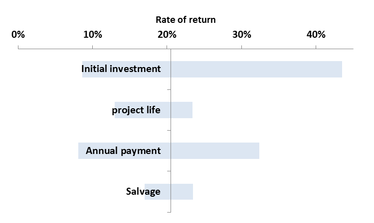
| Type | Rate of Return Range |
|---|---|
| Initial investment | 8.6% - 43.5% |
| Project life | 13% - 23.4% |
| Annual payment | 8.1% - 32.4% |
| Salvage | 17% - 23.5% |
Please watch the following video (18:02): Sensitivity Analysis.
PRESENTER:
In this video, I will work on an example and explain the sensitivity analysis method. I will describe how we can use this method for project evaluation. Let's work on a simple example.
In this example, we will run single variable sensitivity analysis. We also assume all the input variables are independent and have no effect on each other. For instance, we assume the magnitude of initial investment has no effect on operating costs.
This investing project requires $150,000 of investment at the present time and it yields the annual income of $40,000 for five years from year one to year five and the salvage value of $80,000 in the end of the year five. And we want to evaluate the sensitivity of the project rate of return to 20% and 40%, change increase and decrease in initial investment, annual income, project life, and salvage.
First we calculate the rate of return on this cash flow for this project. The present value of costs equals present value of income plus present value of salvage. And we will find that we will solve this equation for i using the IRR function in Excel or any other spreadsheet. And we calculate the rate of return on this cash flow as 20.5%.
First, sensitivity analysis of initial investment. So in the first step, we want to see what would be the rate of return for this project if we decrease the initial investment by 40%. It means we have to multiply this under $50,000 by 1 minus 40%. So it is going to be $90,000. So if the initial investment of the project decreases by 40%, then we will have the initial investment of $90,000 at present time.
And we calculate the rate of return for this new situation. Present value of cost equals present value of income plus present value of salvage. And we calculate the rate of return as 43.5%.
Now effect of 20% decrease in the initial investment. So the initial investment, if it is decreased by 20%, is going to be 1 minus 20%, multiply $150,000. And we calculate the rate of return for the new situation, for the case that we have 20% less initial investment. And the rate of return is going to be 29.6%.
The third case is when we calculate the rate of return for a 20% increase in initial investment. So initial investment is going to be 1 plus 20%, multiply $150,000, which is going to be $180,000 of investment. And the rate of return can be calculated as present value of cost equals present value of income plus present value of salvage. And the rate of return will be 13.8% if the initial investment is increased by 20%.
And the fourth case is when our initial investment is increased by 40%, which is going to be 1 plus 40%, multiply $150,000, which comes to $210,000. And the rate of return is calculated as 8.6% if the initial investment is increased by 40%.
And this table summarizes the result for sensitivity analysis on initial investment. So the third row is the base case when there is no change in our initial investment. The rate of return, as we calculated, was 20.5%. If the initial investment is decreased by 40%, then the rate of return for this project is going to be 43.5%, which will be 112.7% higher than the base case that we had.
Initial investment is decreased by 20%, then the rate of return is going to be 29.6%, which, comparing to the base case, the rate of return is going to be 44.8% higher than the base case. If the initial investment is increased by 20%, then rate of return is going to be 13.8, which is going to be around 33% lower than the base case. And the last case, if the initial investment is increased by 40%, then the rate of return for the project is going to drop to 8.6%, which is 58% lower than the base case that we had.
Now let's do the sensitivity analysis for the project lifetime. The project lifetime is initially five years. So the 40% decrease in project lifetime is going to be 1 minus 40, multiply 5, which is going to be three years. So the project with the initial investment of-- we hold every other thing constant. So the project with initial investment of $150,000 and annual income of $40,000 for three years and the salvage value of $80,000. We calculate the rate of return, which is going to be 12.9%.
And then effects of a 20% decrease in project lifetime. So if the project lifetime is decreased by 20%, you're going to have four years, 1 minus 20% multiply by five, which comes to four. And a calculation of rate of return for the new cash flow, we're going to have four years of income of $40,000. And rate of return is going to be 17.7%
Of 20% increase in project life, which is going to be 1 plus 20%, multiply 5, which is going to be 6 year. One year increase in project lifetime, in this case, we are going to have a rate of return of 22.2%. And if the project lifetime is increased by 40%, meaning that we add two more years to the lifetime of the project, one plus 0.4, multiply 5, equals to 7. We have two more years of project lifetime. And the rate of return can be calculated as 23.4.
And we summarize the sensitivity analysis of project life result in this table. So the third row is the base case. Project life is initially five years. And the rate of return is 20.5%.
If the project life is decreased by 40%, we are going to have three years of project life and the rate of return is going to be 12.9%. If the project life is decreased by 20%, then the rate of return is going to be 17.7%, which is 13.5% less than the base case. If the project life is increased by 20%, then we can see it is going to have positive impact on the rate of return, which is 8.7% higher than the base case, higher than 20.5%. And if the project lifetime is increased by 40%, the project life is going to be seven years and the rate of return is going to be 23.4, which is 14.5% higher than the base case, which was 20.5%.
And now sensitivity analysis for annual income. The initial value for annual income was $40,000. 40% decrease means 1 minus 40%, multiply $40,000, and we're going to have the annual income of $24,000. We calculate the rate of return for such projects. So every other thing is the same. We just decrease the annual income by 40%. So the rate of return is going to be 8.1%. [AUDIO OUT].
The effect of 20% decrease in annual income will be 1 minus 20%, multiply $40,000, which is going to be $32,000. We're going to have $32,000 if the annual income is decreased by 20%. And the rate of return for such project is going to be 14.3%.
We will repeat these calculations for 20% increase in annual income. If annual income from the base case is increased by 20%, we are going to have 1 plus 20%, multiply $40,000, which gives $48,000 of annual income per year for five years. And the rate of return is going to be 26.5%.
We'll repeat the calculations for a 40% increase in annual income, which is going to be 1 plus 40%, multiply $40,000, which comes to $56,000 annual income. So if our annual income is increased by 40% from the base case, we are going to have $46,000 per year. And the rate of return in this new case will be 32.4%.
So, again, this table summarizes the sensitivity analysis of annual income. The base case is when we have $40,000 of income per year. The rate of return is going to be 20.5%. If the annual income is decreased by 40%, we are going to have $24,000 per year and the rate of return is going to be 8.1%, which is going to be 60.6% lower than the base case, lower than the base case of 20.5%.
If the annual income is decreased by 20%, we are going to have $32,000 per year and the rate of return is going to be 14.3%, which is almost 30% less than the base case. If annual income is increased by 20%, we are going to have $48,000 dollars per year and the rate of return is going to be increased to 26.5%, which is 29.5% percent higher than the base case. And in the end, if annual income is increased by 40%, we will have the annual income of $56,000. And rate of return is going to be 32.4%, which is 58.5% percent higher than the base case.
And the last part, we are on the sensitivity analysis for the salvage value. The initial value for salvage is $80,000. 40% decrease in salvage value can be calculated as 1 minus 40%, multiply $80,000, which comes to $48,000. And the rate of return for this change, $40,000 of salvage, which is here, is going to be 17%.
We'll repeat the calculations for 20% decrease in salvage. 1 minus 20%, multiply $80,000, which is going to be $64,000 of salvage. And the rate of return, 18.8%. Percent.
We will calculate this for 20% increase in salvage. 1 plus 20%, multiply $80,000 equals $96,000. And the rate of return can be calculated as 22%. And the last one, 40% increase in salvage value, which will be 1 plus 40%, multiply $80,000, equals \$112,000 of salvage value. And rate of return will be 23.5.
This table summarizes the sensitivity analysis of salvage value. The third row is the base case. There is no change in any input variable and the rate of return is 20.5%.
The first row is the case that we have 40% decrease in salvage value. In this case, the rate of return is going to be 17%, which is 17% lower than the base case, which was 20.5%. If the salvage value is decreased by 20%, then rate of return is going to be 18.8%, which is 8.2% lower than the base case.
If the salvage value is increased by 20%, the rate of return is going to be 22%, which is 7% higher than the base case. Last row, which shows the 40% increase in salvage. And the rate of return in this case is going to be 23.5%, which is almost 15% higher than the base case of 20.5%.
This table summarizes the sensitivity analysis result for these four input variables. So the second row is the base case where nothing has changed. So rate of return is 20.5%.
The first row shows if the input is decreased by 40%. So if the initial investment is decreased by 40%, then rate of return is going to be 43.5%. If the project lifetime is decreased by 40%, we can see it has a negative effect on the rate of return. The rate of return is going to decrease to 12.9% and so on.
The last row shows the result if the input variable is increased by 40%. So if the initial investment is increased by 40%, rate of return is going to be 8.6%. If the project life is increased by 40%, rate of return is going to be 23.4 and so on.
We can also summarize these results in a graph called tornado graph. And we can see here this vertical line shows the base case where nothing has changed. The rate of return is 20.5%. This bar shows what would be the change in the rate of return of the project if initial investment changes from 40% positive to 40% negative, 40% increase to 40% decrease.
Credit: Farid Tayari
If you are interested, the following video (10:48) explains how to draw a tornado chart in Microsoft Excel (please watch from 6:10 to 9:00).
CHARLIE NUTTELMAN: This screencast is going to go over a sensitivity analysis, and we're going to generate a tornado plot. A sensitivity analysis is basically a study into how sensitive is the process, so the process outputs, to the inputs. So just as an example here, we have a process, and it's got a bunch of inputs, and it may have one or more outputs.
An example might be a reactor where the inputs would be things like the temperature, the pressure, maybe the size, the flow rate, concentration of different things, and so on. And the outputs might be conversion. Just a simple example. And we want to determine how sensitive the outputs of the process are to the inputs.
The specific example I'm going to be working with has to do with net present value. We've made a screencast on this already, and you don't necessarily have to understand this net present value example. It has to do with engineering economics and determining the net present value of a venture 15 years from the current time. We have different inputs to the process. The inputs would be things like the cost of land, the cost of royalties per year, the total depreciable capital-- that's how much you have to invest in major equipment-- working capital, startup costs.
We have sales, which is S. Other inputs include tax, because tax rates might change. And cost of sales, here we have 6 million. And we have an interest rate, or the cost of capital. So again, you don't necessarily have to understand exactly what I've done in this spreadsheet to understand sensitivity analysis. The important thing is that we have a process and we have multiple inputs that go into determining what the output is. And for this process, the output is down here.
This tells us that the net present value of a venture based upon our base case, or our baseline or nominal values of these different variables up here, the net present value that is about 58 million. We're going to now do a sensitivity analysis. We're going to see what happens when we change different values here for the cost of land, maybe the annual sales, and annual costs, and so on. So what happens, maybe, if we subtract 20% from the nominal values and increase 20%?
So you'll notice here, I have 58.78 million down here. And if I change something like cost of sales, let's just say to eight, instead of being 58.78, it's a lot less. It's 50.30. So you can see that this process, the output which is net present value, depends upon the input variable. So I'm going to put that back to six. And maybe I change land to instead of 5 million, it's negative 4 million but that didn't change it a whole lot. It was 58.78, and now it's 59.78. So I'm going to put that back to minus five.
We're going to do a data table to look at these different input variables and what effect they have on the output. So we're going to do a sensitivity analysis first on the working capital. The nominal value, or the baseline value, for working capital is negative 20 million. That's how much we're going to request for working capital. And we want to ask ourselves how sensitive is the net present value after 15 years? How sensitive is that to the working capital? So if we have 80%, that'd be minus 16 instead of minus 20, as opposed to 120%, which is negative 24.
So all I've done here is multiply our baseline value of negative 20, which is up here in our spreadsheet. I multiplied that by 80%, all the way up to 120%.
We're going to make a data table here. When you make a data table, we have a column of different inputs that we're going to do kind of a case study on, the cell one up and one over from our values. This is a pointer formula, so I'm going to do equals. We're pointing to our net present value. That's the result. And then what I can do is highlight all of this, our column of cells, plus one row above. And I'm going to go into Data, What If Analysis, Data Table. And this is a column data table. And each of these working capital values is going to be placed into cell B4 up here.
And so I'm going to press OK, and it's going to do sort of a case study on that. I forgot to mention one thing. If I just did a multiplication of cell C33 here, which is negative 20, times the percentage and created a vector here, I actually have to copy and paste so that's not a formula. Because if this is a formula and we put that into the data table, it doesn't quite work right. So we have to copy and paste the values so they're just numbers instead of formulas in this column before we do the data table.
So this is telling us if the working capital is negative 16, the net present value is about 62.5 million. And if we increase it by 20%, we see that the net present value is about 55 million. So I can go through all of these different values. And the green here represents the baseline values. So we have working capital, which I showed you. I did this for startup costs, sales, the interest rate or cost of capital, the land costs, total depreciable capital, capital, and cost of sales.
And what I've done for all of these, I've taken the minus 20, which is our 80% of nominal cost, and our 120% of that particular variable and I've made a summary table here. What we're going to do now is create something known as a tornado plot. To create the tornado plot, I'm going to highlight one of these rows. I go up here to Insert, Chart, and we're making a clustered chart, a clustered bar chart. And right now, it's not looking anything like a tornado plot, but bear with me here.
I'm going to format this a little. I'm going to go over here and add in axis titles. I'm going to add in a legend. I'm going to go back up here, and I'm going to copy, so I'm selecting this, Control + C. That's the 120%. And I'm going to click in the area, do Control paste. Now, again, this isn't looking really like a tornado plot, but we have some work to do. We need to change this. I'm going to do Format Axis, and it's going to cross axis values. Vertical axis crosses axis value at 58.78. That was our nominal value.
So if I go back up here, 58.78 is the net present value when we have 100% of all those values. That was our base case. Now this is sort of looking like a tornado diagram. And I'm going to click on one of these series, Format Data Series. We're going to do 100% overlap, sort of eclipsing. And I'm going to make this a little bigger. I'm going to decrease the gap width, maybe something around 60%.
We can further modify this. So I'm going to right-click on this axis, Format Axis. Let's change the number to be zero decimals. I'm also going to click on the category over here, and we will format that. So I'd right-click on this, format that axis. I'm going to change the labels so they are low. What that does is it brings those labels to the left side.
And another thing I'm going to do is change those labels. So I'm going to do Select Data. Instead of these one, two, through eight, I'm going to edit that, and that's going to be named our categories up here. So I can do that. Click OK. And it has added those different categories.
And the last thing we need to do is to change our legend. So I'm going to bring the legend inside here so I can expand this a tiny bit. And I can right-click in here and do Select Data. And I'm going to change this to minus 20%. I'm editing the series, and this will be plus 20%. And we're pretty much done. So that is a tornado diagram.
And what this tornado plot shows us is that if we change, for example, sales, if that goes down by 20% of our baseline, then that has a huge effect on the net present value. Same thing with if we increase sales by 20%. That has a very big effect on net present value. Some other things that don't have as big of effect, you see that C_land doesn't have a big effect. If your land costs vary tremendously, that's not going to have a huge effect on net present value at all. But if your sales are off of what you're anticipating, then this can have a huge effect on the net present value.
So that's varying from around 20 million to 100 million, which is a huge difference there. And your boss might say, if you gave him this sensitivity plot, your boss might say, well, we need to put a lot more effort into making sure we have a really good estimate on sales. Because if sales are 20% lower than what we're expecting, then the profitability of this venture's way lower than if our sales are 20% higher than what we're expecting.
This sort of tells you what are the main players in your output, and the output, in this case, is net present value. And if you really wanted to, you could organize this. You can put the big bars up at the top and the small ones at the bottom, and it sort of looks like a tornado, so that's what the tornado plot gets its name. OK, thanks for watching this screencast.
Expected Value Analysis (Economic Risk Analysis)
The expected value is defined as the difference between expected profits and expected costs. Expected profit is the probability of receiving a certain profit times the profit, and the expected cost is the probability that a certain cost will be incurred times the cost.
Example 6-2:
A wheel of fortune in a gambling casino has 54 different slots in which the wheel pointer can stop. Four of the 54 slots contain the number 9. For a 1 dollar bet on hitting a 9, if he or she succeeds, the gambler wins 10 dollars plus the return of the 1 dollar bet. What is the expected value of this gambling game? What is the meaning of the expected value result?
- 0.185 dollars indicates that if the gambler plays this game over and over again, the average gain for the gambler per bet equals - 0.185 dollars, which means the gambler will lose 0.185 dollars per bet. Note that for a satisfactory investment, a positive expected value is a necessary, but not sufficient, condition.
Example 6-3:
Assume drilling a well costs 400,000 dollars. There are three probable outcomes:
a) 70% probability that the drilled well is a dry hole
b) 25% probability that the drilled well is a producer well with such rate that can be sold immediately at 2,500,000 dollars
c) 5% probability that the drilled well is a producer well with such rate that can be sold immediately at 4,000,000 dollars
Calculate the project's expected value.
Note that +425,000 dollars is a statistical term; it means the average of +425,000 dollars will be achieved in the long-term for drilling over and over again in a repeated investment of this type.
Expected NPV and Expected ROR Analysis
Example 6-4:
Assume a research project that has the initial investment cost of 100,000 dollars. There are two possible outcomes:
a) 30 % success: that leads to an annual profit of 60,000 dollars for five years (starting from year 1) with a salvage value of zero
b) 70 % failure: that leads to annual profit and salvage value of zero
Considering a minimum 12% discount rate, compare the expected NPV, and explain if this investment is satisfactory.
| 30 % success: | -$100,000 | $60,000 | $60,000 | $60,000 | $60,000 | $60,000 |
| 70 % failure: | -$100,000 | 0 | 0 | 0 | 0 | |
|
|
||||||
| 0 | 1 | 2 | 3 | 4 | 5 | |
Since considering risk in calculations results in negative expected Net Present Value (ENPV), it can be concluded that this investment is expected to be economically unsatisfactory. Note that risk-free NPV (assuming 100% success probability) shows good and economically satisfactory results.
Example 6-5:
Calculate the expected Rate of Return for the above example.
Expected ROR is the “i” that makes Expected NPV equal 0.
Expected Present worth income @ "i" – Present Worth Cost @"i" = 0
By trial and error, Expected ROR = - 3.4%
Note that risk free ROR shows a satisfactory result.
Risk-free ROR = 52.8%, which is much higher than the minimum ROR.
Another way to calculate the expected ROR, which is similar to the previous method, is to calculate expected cash flow and then find the ROR for that.
Expected cash flow can be determined by multiplying each scenario’s cash flow by its probability and then make summation over each year:
| Year 1 | Year 2 | Year 3 | Year 4 | Year 5 | |
|---|---|---|---|---|---|
| Expected cash flow |
Then:
| Year 1 | Year 2 | Year 3 | Year 4 | Year 5 | |
|---|---|---|---|---|---|
| Expected cash flow | -$100,000 | $18,000 | $18,000 | $18,000 | $18,000 |
By trial and error, Expected ROR = - 3.4%
Please watch the following video (14:01): Expected Value Analysis, Part I.
PRESENTER: In this video, I will explain the second method to incorporate risk and uncertainty in project evaluations. This method is called expected value analysis, and the expected value is the difference between expected profits and expected costs. Expected profit is the probability of receiving a profit multiplied by the profit, by the payoff, and the expected cost is the probability that certain costs will be incurred multiplied by that cost.
Let's assume a wheel of fortune that has 24 slots, and three of these slots have a red color. So you randomly turn this wheel of a slot, and if you get a red color, you will win $5. And if you get any color other than red, you will lose $1. So let's see what would be the expected value of this game and what is the meaning of the expected value results?
So the probability of success is 3/24, and the probability of failure is going to be 21 divided by 24. So the expected value equals the expected value of profit minus the expected value of cost. The expected value of this game is minus $0.25. So it means that if we play this game over and over again, the average gain per bet, the average gain per game, is going to be $0.25. So if we play this game over and over again, we will lose $0.25 per game.
Let's work on this example. Assume a drilling well that costs $400,000, and there are three possible outcomes. We have a 70% probability that we get a dry hole, which means there will be no outcome and we just have the cost of $400,000 at the present time. There is a 25% probability of success that we get a producer well, which can be immediately sold at a price of $2.5 million. And we have a 5% probability that we drill a well that is a producer and can be sold immediately at $4 million.
Let's calculate the project's expected value. So this is the expected value of failure, 70% multiplied by we have just $400,000 of cost. There is no income revenue or profit, in this case. And we have two cases of success. We have 25% of success that we get a producer well and we can sell it at $2.5 million, but we still have the $400,000 of costs. And also, we have another success case with a probability of 5% that is going to yield $4 million of immediate income, and we have $400,000 of drilling cost.
And the summation is going to be $425,000, the expected value of this project. So in each case, we multiply the probability of that event by the outcome of that event. So this is the outcome. This is the failure case. This is the outcome of the failure, and this is the probability. Here, this is one of the success cases. This is a 25% probability of success. And in case of success, we are going to have $2.5 million, but still, we have to pay the drilling cost and so on.
Please note that the $425,000 of expected value for this project is a statistical term, and it means that the average of $425,000 will be achieved in the long term. If we do this drilling, if we play this game, if we drill this field over and over again, holding the probabilities and costs and incomes constant, this is the expected value that we are going to achieve after doing the drilling again, over and over again.
Another example. Let's assume an investment project requires the initial investment cost of $100,000, and there are two possible outcomes. There is 30% of success that leads to an annual profit of $60,000 for five years, equal payments of $60,000 for five years. The salvage value is going to be zero. And the 70% failure that we receive nothing. There is no annual profit, and salvage would be zero.
Let's calculate the expected NPV for this project, assuming the minimum discount rate of 12%. So we draw these two cases in the timeline. There is 30% of success that we have $100,000 of cost at the present time. And in this case of success, we are going to have a $60,000 annual income of $60,000 per year from year one to year five. In case of failure, we still need to pay the initial costs for this project, but we will earn nothing in the future years.
So in this case, we need to calculate the NPV of each case, multiply that by the probability, and then make a summation over all the possible cases. So here we have a 30% probability of success. This is the NPV of success. This shows the NPV of success. We have $100,000 of cost at the present time, and we have five equal payments of $60,000 from year one to year five.
Probability of failure. Multiply the failure case, NPV of failure, which is going to be just the $100,000 of cost at the present time, and the expected NPV for this project, which is a negative value.
So if we consider risk in this project, meaning that we are assuming a 30% probability for success and 70% probability for failure, we are going to have expected-- We are going to have negative expected NPV, which means that this project is not a good project for investment. Note that the risk-free NPV, meaning that the probability of success is 100%, is going to be a positive number, which means this project is economically satisfactory.
Now, let's calculate the expected rate of return for this example. Again, the example is the same. We have a project that requires $100,000 of investment at the present time. There is 30% of success that yields $60,000 of income for five years from year one to year five, and there is a 70% of failure that we will earn nothing, the annual profit, and the salvage value will be zero.
So the expected rate of return is the rate that makes the expected NPV equal zero. So the equation for expected rate of return is expected present value of incoming equals expected present value of cost. So in case of success, we are going to have $60,000 for five years. And the probability is the present value of the $60,000, and this is when we multiply that with the probability of success, it gives us the expected present value of income.
And on the right-hand side, we are going to have the expected value of cost, which is going to be $100,000 if we have in case of success, multiplied by the probability of success. And also, plus $100,000 in case of failure, multiplied by the probability of failure. And you can see because this cost is shared between these two cases, so it stays unchanged. Because the decimation of this probability equals, these two probabilities equal one. So the expected present value of income equals the expected present value of cost and solving this equation for i, we'll get the rate of return of minus 3.4%.
There is another way to calculate the expected rate of return for this project, which we can calculate the expected rate of return from the expected cash flow. How do we calculate the expected cash flow for each year, for each column? We calculate the expected money that will happen in that year. For example, this year, we have $100,000 of investment with a probability of 30% plus $100,000 of investment at a probability of 70% failure and for the year one, we are going to have $60,000 of income. But the probability of this income is going to be 30%. So $60,000 multiplied by 30%.
And we have zero income with a probability of 70%, which I didn't write it here because it equals zero. And same for the other years. And we calculate the summation. So in each year, we write the expected cash flow. We write the expected money that is going to happen in that year. For year one, we are going to have the $100,000 of investment. Again, because this investment is shared, is common for both failure and success, it stays unchanged. But for the other years, because we have income only for the success scenario, we multiply the $60,000 of income by 30%. And we are going to have $18,000 for the year one to year five.
So we can calculate the rate of return, the same as what we used to do for cash flow. It might be easier to just write the rate of return equation for this cash flow. We have $100,000 of costs, and we have $18,000 of income from year one to year five. The present value of cost equals the present value of income. And we solve this equation using Excel or any other spreadsheet.
Example 6-6:
Calculate Expected NPV for a minimum ROR 20% to evaluate the economic potential of buying and drilling an oil lease with the following estimated cost, revenues, and success probabilities.
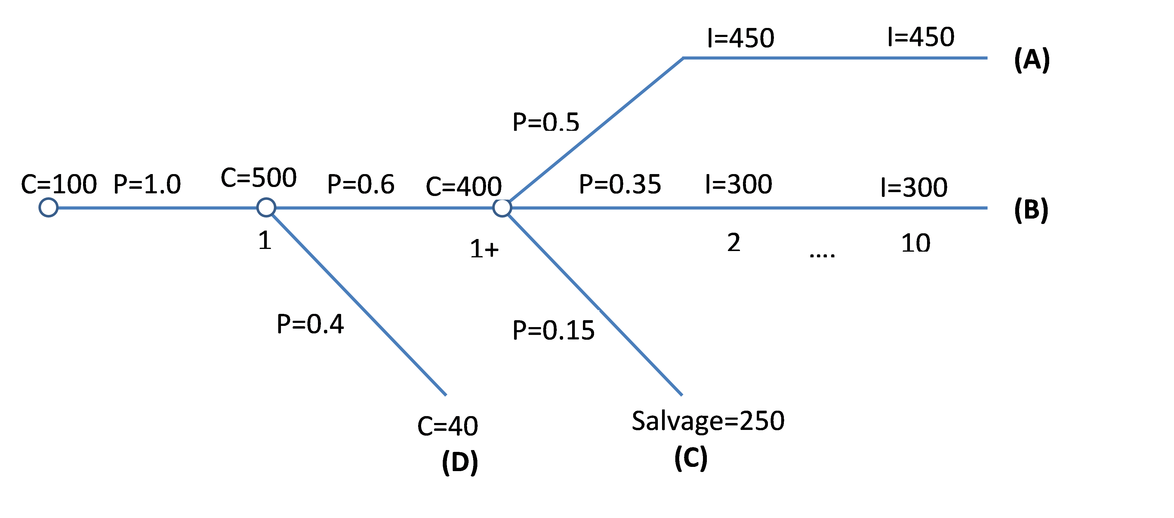
The lease would cost 100,000 dollars at time zero and it is considered 100% certain that a well would be drilled to the point of completion one year later for a cost of 500,000 dollars. There is a 60% probability that well logs look good enough to complete the well at year 1 for a 400,000 dollar competition cost. If the well logs are unsatisfactory, an abandonment cost of 40,000 dollars will be incurred at year 1. If the well is completed, it is estimated there will be a 50% probability of generating production that will give 450,000 dollars per year net income for years 2 through 10 and a 35% probability of generating 300,000 dollars per year net income for years 2 through 10, with a 15% probability of the well completion being unsuccessful, due to water or unforeseen completion difficulties, giving a year 2 salvage value of 250,000 dollars for producing equipment.
The above decision-making process can be displayed in the following figure. These types of graphs are called decision trees and are very useful for risk involved decisions. Each circle indicates a chance or probability node, which is the point at which situations deviate from one another. (Costs are shown in thousands of dollars.)
Note: Times 1 and +1 are the same points in time and both indicate the end of year 1. The main body (of the tree) starts from the first node on the left with a time zero lease cost of 100,000 dollars that is common between all four situations. The next node, moving to the right, is the node that includes a common drilling cost of 500,000 dollars. At this node, an unsatisfactory and abandonment situation with a cost of 40,000 dollars in the first year (situation D) deviates from other situations (a branch for situation D deviates from the tree main body). The next node on the right (third node) is the node where situations A, B, and C (three separate branches) get separated from each other. At the beginning of each branch is the probability of that situation, and at the end of it, amounts due to that situation (including cost, income, and salvage value) are displayed.
So, there are four stations:
Situation A: Successful development that yields the income of 450 dollars per year
Situation B: Successful development that yields the income of 300 dollars per year
Situation C: Failure that yields a salvage value of 250 dollars at the end of year two
Situation D: Failure that yields abandonment cost of 40 dollars at the end of year one
Probability of situation A can be calculated as
Probability of situation B can be calculated as
Probability of situation C can be calculated as
Probability of situation D can be calculated as
| Probability | |||||||
| A) |
0.3
|
C=$100 | C=$500+$400 | I=$450 | I=$450 | ... | I=$450 |
| B) |
0.21
|
C=$100 | C=$500+$400 | I=$300 | I=$300 | ... | I=$300 |
| C) |
0.09
|
C=$100 | C=$500+$400 | Salvage=$250 | 0 | ... | 0 |
| D) | 0.4 | C=$100 | C=$500+$40 | 0 | 0 | ... | 0 |
|
|
|||||||
| 0 | 1 | 2 | 3 | ... | 10 | ||
Note that the summation of all properties should equal 1.
Project ENPV is the summation of ENPV for all situations. So, first, we need to calculate ENPV for each situation:
And it can be summarized in Table 6-1 as:
| Probability | Year 1 | Year 2 | Year 3 | Year 4 | ... | Year 5 | ENPV | |
|---|---|---|---|---|---|---|---|---|
| A | 0.3 | -$100 | -$900 | $450 | $450 | ... | $450 | $198.5 |
| B | 0.21 | -$100 | -$900 | $300 | $300 | ... | $300 | $33.1 |
| C | 0.09 | -$100 | -$900 | $250 | 0 | ... | 0 | -$60.9 |
| D | 0.4 | -$100 | -$540 | 0 | 0 | ... | 0 | -$220 |
Project ENPV is slightly less than zero compared to the total project cost of 1 million dollars, therefore, slightly unsatisfactory or breakeven economics are indicated.
Please watch the following video (13:32): Expected Value Analysis, Part 2.
PRESENTER: Let's work on a more complicated example. Let's assume a drilling project.
The lease costs would be $100,000 at time 0. That will be paid for all the cases. Then we will have the $500,000 of drilling costs at year 1. Again, this cost is paid for all the cases.
After we paid these $500,000 of drilling costs, we get to the completion point. At this point, there is 60% probability that well logs are good enough to complete the well, which is going to cost $400,000. And there is a 40% failure that they don't look good enough. And we need to close the wells and pay the abandonment cost and so on.
So in case of the 60% probability, let's call it a success case, we will pay $400,000 more in the same year 1 for completion costs. In this case, we will face three cases. One case with a probability of 50%, we will have a producer well, which is going to produce $450,000 per year of income from year 2 to year 10.
And the second case, we are going to have a 35% probability of a well that is going to generate $300,000 per year from year 2 to year 10. And we will have a 15% probability of that the well completion being unsuccessful. And we will have a salvage value of $250,000 for producing equipment in year 2.
So we can summarize the information here. There will be $100,000 of lease costs for all the cases at the present time. And there will be $500,000 of drilling cost at year 1 for all the cases. And then we'll have a 60% probability of getting to the completion. In this case, we pay another $400,000 in year 1. And if I weight 40% probability if we don't complete the well, we need to pay and order $40,000 of costs at year 1.
So in the case of 60%, we will face three new cases. 50% probability that generates $450,000 from year 2 to year 10. And case two, 35% probability of generating $300,000 from year 2 to year 10. And a 15% probability that we don't end up doing anything, any money, any producing well. And we have just a salvage value of $250,000 in year 2.
So the decision tree is a very helpful graph that can help us separate the possible cases here. So I will explain this in this graph. So we start from the left-hand side, the initial investment for the lease at the present time. We write the cost or income here. And in front of that, we write the probability.
So this probability is 100% because it is the same for all the cases. At year 1, we spend $500,000 for drilling, and then, in this case, we are going to have two branches being deviated from the main branch. One is 60%, let's call it a success here, a 60% probability of success and a 40% probability of failure. In case of failure, we are going to pay $40,000 of closing costs, abandonment costs.
In case of success, 60%, we will face another three cases. In case of success, we will pay another $400,000 of completion costs. This 1 plus is to show that this is the same year as this year. These are happening in the same year. But because these cases deviate from the main branch, we draw another branch for these, to separate these from the main branch.
So 60% of success, we pay $400,000 of completion cost. And we will have three new cases in the after. So there is a 50% chance, there is a 50% probability that we will earn $450,000 from year 2 to year 10. So years are here.
So every value under the same column has the same year dimension. We have 35% of getting $300,000 from year 2 to year 10. And we have a 15% probability that we get only $250,000 of salvage at year 2.
So as we can see here, we have four main cases here. Case A, case B, case C, and case D. So the first step to approach this problem and calculate the expected NPV is to calculate the probability of each case. So in order to calculate the probabilities of each case, we go back to the decision tree.
We start from the right-hand side for each case. For example, for case A. So I start from the right-hand side. For example, case A, I start moving from the right-hand side toward the left.
I have a 50% probability here. And go to the main branch. I have a 60% probability here. And I have a 100% probability here. So I will multiply.
I start moving from the right-hand side along each branch to the left, and I multiply the probabilities that I see on the way. So here, I have a 50%, and 60% probability, and a 100%. So I will multiply 50% multiply 60% probability and 100% which has no effect. So the probability of A is 50% multiplied 60%.
B, the probability of case B is 35%, multiply 60%. And multiply this 100%, which has no effect. Case C, probability of 15%, multiply 60%. And case D, the probability of 40% multiply 1, which is going to be 40%. So I calculate the probabilities for case A, case B, case C, and case D.
In the second step, I draw the timeline and I separate the cases from each other. In the first row I write the probabilities. Case A, there is a $100,000 lease cost at the present time. Drilling costs at year 1, plus $400,000 of completion costs.
You remember this was in case the well logs look good. So this $400,000 happens in the same year. And case A is going to generate $450,000 from year 2 to year 10.
Case B, $100,000 of lease costs, plus $500,000 of drilling, plus $400,000 of completion costs. This was happening in year 1. The lease cost is at year 0. And the income from year 2 to year 10.
Case 3. Case 3, the lease cost, the drilling costs, and the completion costs are $400,000 in year 1. And I'm going to have just the salvage of $250,000 in year 2. And the income for other years is going to be 0.
So in case D, which I call it failure case. I pay the lease cost at the present time. I pay the drilling cost in year 1. But the well logs are not looking good enough to pay the completion costs. So I will just close the well and pay the abandonment cost of $40,000.
So now that I have this table calculating the expected NPV. For each case, I calculate the NPV and I multiply that by the probability. And I make a summation over all that.
So here, you can see this is the equation for case A to calculate the NPV. This is the lease cost at the present time. It doesn't need to be discounted.
This is the summation of $500,000 of drilling cost, plus $400,000 of the completion costs. And the $450,000 of income from year 2 to year 10, which they are 9 equal series of income payments. And I need to discount this for one year because they start from year 2.
And the NPV for case B, case C, and case D. Please note that the salvage is happening at year 2 for case C, so I need to discuss that for two years. And I write the NPV for each case in the last column. I multiplied probability by the NPV for each case. And I wrote that too in this column.
And the summation of all these values here is going to give me the expected NPV for this project. And as you can see here, it is going to be about minus $50,000. And the conclusion would be because the expected NPV is slightly negative, is slightly less than 0. We can conclude that this project is not very economically satisfactory.
Credit: Farid Tayari
Italicized sections are from Stermole, F.J., Stermole, J.M. (2014) Economic Evaluation and Investment Decision Methods, 14 edition. Lakewood, Colorado: Investment Evaluations Co.
Risk due to Natural Disaster
One method used to analyze the uncertainty and risk involved in natural disaster decision makings is to choose the best alternative base on the lowest expected cost. In the following example, you can practice this method.
Example 6-7:
A company is planning to build a new plant. The plant requires water for its production process and needs to be built near a river. But the location has the probability of being flooded and building levees around the plant is necessary to protect the facility. There are four possible sizes of levee that have different costs, maintenance, and level of protection, as displayed in following table. Calculate the expected annualized cost for each levee, considering minimum ROR of 12% and 18 years project life. Then explain which levee has the lowest expected annualized cost for the company.
| Levee size | Levee Cost | Probability that levee fails | Expected Damage | Annual maintenance |
|---|---|---|---|---|
| 1 | $150,000 | 0.25 | $100,000 | $3,000 |
| 2 | $180,000 | 0.15 | $130,000 | $4,500 |
| 3 | $200,000 | 0.08 | $140,000 | $5,000 |
| 4 | $220,000 | 0.04 | $180,000 | $7,000 |
Probability of levee failure: Probability of a flood exceeding levee size during the year
Expected Damage: Expected damage if flood exceeds levee size
In order to calculate expected annualized cost for each levee size, we need to convert all the costs into annual base. Then:
From Table 1-12, equivalent annualized levee cost can be calculated as:
Expected damage per year is the multiplication of Probability of levee fails by Expected Damage
Expected annualized cost for different sizes of levee can be calculated as:
| Levee size | Annual Levee Cost | Expected damage per year | Annual maintenance | Expected annual cost |
|---|---|---|---|---|
| 1 | $20690.59 | $25,000 | $3000 | $48,690.59 |
| 2 | $24828.72 | $19,500 | $4500 | $48,828.72 |
| 3 | $27587.46 | $11,200 | $5000 | $43,787.46 |
| 4 | $30346.21 | $7,200 | $7000 | $44,546.21 |
Results show that the third levee has the lowest expected annualized cost; therefore, it is the best alternative.
Summary and Final Tasks
Summary
Sensitivity analysis is a means of identifying those critical variables that if changed, could considerably impact profitability measures such as rate of return or net present value. Risk analysis identifies the likelihood of project failure and the subsequent cost to the investor.
In this lesson, sensitivity analyses for NPV, ROR, project life, and annual payments are practiced. Expected NPV and ROR are also explained to help analyze the effects of risk and uncertainty on the project economics.
Reminder - Complete all of the Lesson 6 tasks!
You have reached the end of Lesson 6! Double-check the to-do list on the Lesson 6 Overview page [1] to make sure you have completed all of the activities listed there before you begin Lesson 7.