Depreciation Accounting
The term "depreciation" usually refers to the physical degradation of some capital asset, like wear and tear. My car, for example, doesn't drive as smoothly with 120,000 miles on it as it did when it had 12,000 miles. As some piece of capital gets older, you might naturally expect it to be worth less, either because it requires more maintenance or because it cannot be resold for as high a price. (Though the concept of "value" of physical plant can be a bit tricky, as we will learn in the next section.) It is often said that the value of a new car drops by 20% as soon as it is driven off the lot, even though it's basically the same vehicle that was bought for a new-car price. This illustrates the difference that can sometimes arise between physical depreciation and the depreciation in a capital asset's store of value.
Depreciation of an asset's store of value has substantial implications for the financial analysis of energy projects. You might recall from Lesson 5 that the profits of a regulated public utility are determined in large part by its total stock of non-depreciated capital. Who determines the rate at which a power plant, substation or other asset depreciates in value? Similarly, tax authorities in many countries allow companies to "write off" the depreciated value of assets when calculating their total income on which they are subject to paying tax. The term "write off" here refers to a deduction from total taxable income, rather than a deduction in the total tax bill, per se. For example, if you can claim that some capital asset has depreciated in value by $100 over the course of some year, and the tax rate is 35%, then that $100 asset depreciation will ultimately lower your tax bill by $35 (35% of $100), not by $100. This is the difference between a "tax deduction" and a "tax credit." Tax credits will appear later in the course when we discuss financial subsidies for energy projects.
The rate at which an asset is financially depreciated for tax, regulatory, or other financial purposes may be very different than the rate at which the asset actually physically depreciates in value. It is even possible that an asset could be treated as completely depreciated in the eyes of a regulator or the tax authority, yet could still be generating a lot of value for its owner. Many power plants or natural gas mains in the U.S., for example, are several decades old - well beyond their intended 30 to 40 year life spans. These assets are mostly considered to be depreciated assets, yet some continue to be highly profitable.
Depreciation allowances are usually determined by the regulator, tax authority or other relevant oversight body in order to allow the owners of depreciable capital assets to recover the costs of those assets through a series of tax deductions or other gains over the course of some number of years. The idea here is to encourage investment by allowing companies to use investment vehicles to reduce their tax burden. Our discussion here will focus on depreciation allowances that are allowed by tax authorities, since those allowances are ultimately the most important for development of energy project financial statements. The U.S. Internal Revenue Service, if you happen to be interested, maintains a mind-bogglingly complex list of types of property that are eligible for different depreciation schedules and methods. Here is an "introduction" to depreciation from the IRS.
A depreciation schedule lists the percentage of the original (so-called "book") value of a piece of property that can be claimed as a depreciation allowance for tax reporting purposes. Broadly, there are two types of depreciation schedules: straight-line depreciation and so-called accelerated depreciation methods.
Before we get into the mechanics of depreciation, we need to develop some notation.
- P = the up-front cost of the asset;
- F = the salvage value of the asset at the end of its useful life;
- N = the number of years over which the asset will be depreciated;
- A(t) = the depreciation allowance for year t (t = 1,…, N), in percentage terms, such that (i.e., the asset must be fully depreciated over N years);
- D(t) = the depreciation allowance for year t (t = 1,…, N), in dollar terms, so that D(t)=A(t)×P;
- B(t) = the remaining book value of the asset after year t.
Based on these definitions, we can immediately see that B(t) is just equal to the original book value (P) less all of the cumulative depreciation allowances from year 1 to year t. In mathematical terms,
Table 4.5 provides the mathematical formulas for some common depreciation methods. Note that Modified Accelerated Cost Recovery Systems (MACRS), which have become more commonplace, are not included in Table 4.5 but will be discussed below.
| Depreciation Method | D(t) | B(t) |
|---|---|---|
| Straight Line | ||
| Sum of the Year's Digits | ||
| Declining Balance | ||
| Note: | ||
The most straightforward depreciation method is straight-line depreciation. Under straight-line depreciation, the book value of an asset (less its salvage value, if any) can be depreciated evenly over some number of years. For example, if you had an asset with a book value of $1,000; no salvage value; and a ten-year depreciation horizon, you could claim $100 each year for ten years as a depreciation expense and tax deduction.
The other three depreciation methods that we will discuss here - sum of the year's digits, declining balance, and MACRS - are all forms of "accelerated depreciation." Under accelerated depreciation systems, a larger proportion of the asset's book value is allowed to be depreciated in the earlier years of its use, with smaller proportions depreciated in later years of use. This allows the asset owner to enjoy a lower tax burden earlier in the asset's life. Other things being equal, this leads to higher profits in the years immediately following investment. Accelerated depreciation can substantially affect the value of an asset to its owner; we will see later just how this re-allocation of tax burden and profits across the useful life of an asset increases the asset's lifetime benefit to its owner.
The three accelerated depreciation methods that we will illustrate in this lesson are:
- Sum of the Year's Digits (SYD): SYD is best illustrated using a simple example. Suppose that an asset could be depreciated over five years. Then the sum of the digits would be 1+2+3+4+5 = 15. The first year, you could claim 5/15 = 33% of the asset's book value as a depreciation expense, so that A(1) = 33%. The second year, the depreciation allowance would be A(2) = 4/15 = 27%. You can verify for yourself that A(3) = 20%; A(4) = 13%; and A(5) = 7%.
- Declining balance: This could also be called "exponential depreciation" since it depreciates an asset at a constant rate, rather than a constant amount. If an asset is depreciated using the declining balance method over a fixed number of years, the residual book value of the asset is used as the depreciation allowance in the final year. For example, if you had a $100 asset with no salvage value, and were claiming depreciation according to the declining balance system at 25% per year over five years, in the first year your depreciation allowance would be D(1) = 0.25 × $100 = $25. In the second year, you would have D(2) = 0.25 × ($100 - $25) = 0.25 × $75 = $18.75. You can verify for yourself that D(3) = $14.06; D(4) = $10.55, and D(5) = $7.91.
- Modified Accelerated Cost Recovery: MACRS, popular in the United States, is embodied in a series of depreciation tables published by the U.S. Internal Revenue Service. The tables dictate the values of A(t) to be used each year, and also describe which types of assets are eligible for MACRS and over how many years. In other words, different asset types have different values of N and different depreciation schedules A(t). One thing to note about MACRS is that the N-year depreciation schedules actually cover N+1 years (so, for example, five-year MACRS allows depreciation over six years).
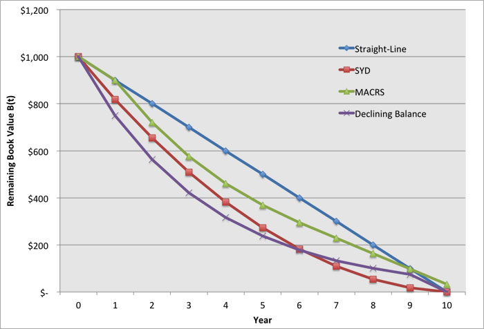
As a means of comparison between all of these methods, let's take a hypothetical asset with a book value of $1,000 and zero salvage value, and depreciate that asset over a ten-year time horizon. Table 4.6 and Figure 4.1 show the values of B(t) during each year for each of the four methods. For declining balance, we will use 25% per year. For MACRS we are using the 10-year table in Appendix 1 of Publication 496.
As an exercise, see if you can reproduce the table and the figure.
| Year | Straight-Line | SYD | MACRS | Balance |
|---|---|---|---|---|
| 0 | $1,000.00 | $1,000.00 | $1,000.00 | $1,000.00 |
| 1 | $900.00 | $818.18 | $900.00 | $750.00 |
| 2 | $800.00 | $654.55 | $720.00 | $562.50 |
| 3 | $700.00 | $509.09 | $576.00 | $421.88 |
| 4 | $600.00 | $381.82 | $460.80 | $316.41 |
| 5 | $500.00 | $272.73 | $368.60 | $237.30 |
| 6 | $400.00 | $181.82 | $294.90 | $177.98 |
| 7 | $300.00 | $109.09 | $229.40 | $133.48 |
| 8 | $200.00 | $54.55 | $163.90 | $100.11 |
| 9 | $100.00 | $18.18 | $98.30 | $75.08 |
| 10 | $ --- | $ --- | $32.70 | $ --- |