
Project Decision Metrics: Net Present Value
Suppose that you were an electric utility considering two potential generation investment opportunities: A natural gas-fired generator with a capital cost of 600 dollars per kW and operating costs of 50 dollars per MWh, or a wind farm with a capital cost of 1,200 dollars per kW and operating costs of 5 dollars per MWh. For the purposes of this example, assume that either power plant could meet the same reliability goals that your utility had. But your regulator wants you to minimize economic costs to consumers. Which should you pick?
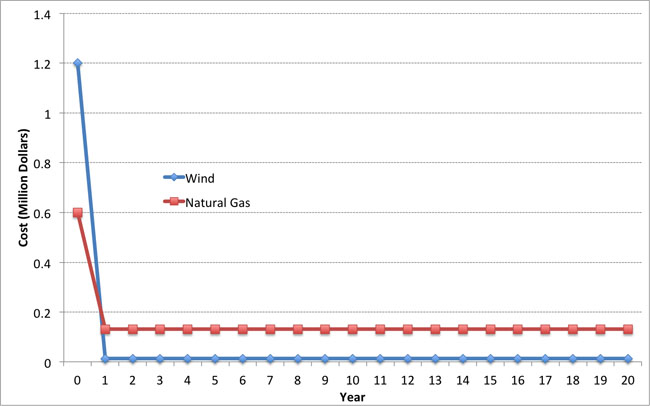
This is a difficult choice because it involves tradeoffs over time. The natural gas generator has a low up-front cost but a higher operating cost. The wind generator has a higher up-front cost but a very low operating cost, because fuel from the wind is free (at the margin). This tradeoff is shown visually in Figure 5.1, for a 1 MW natural gas and wind power plant — for the sake of comparison, we assume that each of the plants operates 30% of the time, so each produces 1 MW × 8,760 × 0.3 = 2,628 MWh per year.
This 30% figure is called the capacity factor, and it measures how much electricity a power plant produces in a year versus how much it could produce each year if it operated all the time at 100% capacity.
Capacity Factor = (Annual Production) ÷ (Capacity × 8,760 hours per year).
Figure 5.1 illustrates the tradeoff but doesn't say much about which decision you should make. Part of the problem is that by investing in the wind turbine, you are accepting a high cost right now in exchange for a stream of operating cost savings in the future. Is this stream of operating cost savings worth it?
One of the most frequently-used metrics to compare projects with different capital and operating cost streams is the net present value, which incorporates the present discounted value of all project costs and revenues.
The net present value (NPV) is defined by two terms: the present discounted value of costs and the present discounted value of revenues. If we let Bt be the (undiscounted) revenues (benefits) of some project during year t and we let Ct be the (undiscounted) costs of the same project during year t, then we can calculate the NPV as follows:
/p>
In the equations, T is the time horizon for the project and r is the discount rate. If the net present value of a project is greater than zero, then the project is said to break even or be "feasible" in present discounted value terms. If you are in a position where you are evaluating multiple alternatives, you would normally want to choose the alternative with the highest net present value.
Sometimes, we will be interested in the net present value of a project as of some year prior to T. We will call this the "Cumulative NPV" as of year X. Mathematically, this is defined as:
Where X is some number smaller than T.
To illustrate, let's go back to one of our examples from earlier in this lesson. Our wind power plant had a capital cost of $1.2 million and annual operations costs of $13,140. Suppose that it had annual revenues of $100,000 and faced a discount rate of 10% per year. Each year, it thus has annual profits of $86,860.
Assuming that all of the capital costs were incurred in Year 0 and the plant began operating in Year 1, the present discounted value of each of the first three years of operation would be:
PV(0) = -$1.2 million (this is just the capital cost, note that this is a negative number)
PV(1) = $86,860÷(1.1)1 = $78,963.64
PV(2) = $86,860÷(1.1)2 = $71,785,12
PV(3) = $86,860÷(1.1)3 = $65,259.20
The Cumulative NPV for the first three years would be:
Cumulative NPV(0) = PV(0) -$1.2 million
Cumulative NPV(1) = PV(0) + PV(1) = -$1.12 million
Cumulative NPV(1) = PV(0) + PV(1) + PV(2) = -$1.05 million
Cumulative NPV(1) = PV(0) + PV(1) + PV(2) + PV(3) = -$983,992
Calculating NPV is reasonably straightforward in a spreadsheet program such as Excel. There are two functions in Excel, PV and NPV, that will calculate net present value for you. The difference between the PV and NPV functions is that the PV function assumes that you have the same profits in each period (as in our example above), while the NPV function does not make this assumption.
The video below shows an example of evaluating NPV using Excel. The example in the video is our natural gas plant from the previous lesson. Registered students can access the Excel file discussed in the video in Canvas.
Video: NPV Example Video (15:19)
So in this video, I'm going to show you how to set up a very simple undiscounted cash flow analysis and calculate a net present value in Excel two different ways. So we're going to go through two different ways of calculating the net present value. One way will be basically by brute force, which will show you how to calculate the present discounted value of costs and benefits in each year. And then you add them up by brute force to get NPV.
The second way is using a built-in function in Excel called the PV function. So we're going to go through both of these. The example or the situation that we're going to use is a power plant. So we have an example of a hypothetical power plant. And it has some capital cost, so some cost to build.
And then once it's built, it has some annual costs in revenues. And so the question is, in present value terms, does this plant make any money? Does this plant pass the cost benefit test? Are the present discounted value of all of the benefits equal-- or all of the revenues, really-- equal to the present discounted value of all of the costs? Or are they bigger, or are they smaller.
So I'm going to start off by typing in some numbers here. And this spreadsheet will also be posted up on Angel if you want to take a look at it. So I'm going to assume that the capital cost is $500,000. So that's how much it costs to build the plant. I'm going to assume that the interest rate here is 10%. I'm going to assume that the relevant decision horizon here is 5 years. So that's the time period over which we're evaluating the profitability of the plant.
I'm going to assume that its annual output is 4,500 megawatt hours of electrical energy. I'm going to assume that its variable cost, so the cost to produce 1 megawatt hour is $60. And so the total annual operating cost, where I here written total variable cost is going to be equal to $60 per megawatt hour times the number of megawatt hours. And so what we get is $270,000 per year. That's how much it costs to operate this plant, assuming that it produces 4,500 megawatt hours each year.
So the sales price for each megawatt hour I assume is going to be $90 per megawatt hour. And so then we can calculate the annual revenue is equal to the sales price, $90 per megawatt hour times the number megawatt hours. And so what we get is annual revenues of $405,000 per year.
The stuff below the cost and revenue figures in the spreadsheet is basically the simple version of the cash flow balance sheet for this power plant. So you have a column for capital cost, a column for operating cost, a column for revenue, a column for the annual undiscounted cash flow, or the net benefit, a column for the discounted cash flow, and then a column here, which I have labeled as cumulative net present value, which will show the overall net present value of this power plant after each year.
And we have year 0, so the current year, all the way down through 5 years from now. So now we have to fill in these table with numbers. So the capital cost we assume is incurred only in year 0. So you only have to spend money this year to build the plant. So that's going to be equal to minus $500,000. You have to be a little careful here when you're doing these things in Excel. You have to be careful that costs are negative numbers and revenues are positive numbers. Otherwise, Excel will mess up your calculations because it doesn't know which one is which.
So this plant has a capital cost of $500,000 in year 0, and that no capital cost in years 1 through 5. So are we going to assume here that the plant is built in year 0 and operates in year 1 through 5. So in each of years 1 through 5, we're going to have an operating cost equal to minus $270,000. And that's going to be the same for each year. Revenues in each year are going to be equal to positive $405,000. and those are going to be the same for each year.
So the annual undiscounted cash flow is going to be the sum of capital cost, operating cost, and revenue for each year. So I'm going to use the sum function here in Excel. Summing over those three columns. In undiscounted terms, this plant costs the owner $500,000 in the first year, and then brings in benefits equal to $135,000 a year for five years.
So now we need to discount this. So remember that to discount some future value back to the present, we take that future value and divide by 1 plus the interest rate raised to the t-th power, where t is the year that we're talking about. So we're going to take this and divide it by 1 plus-- and I'm going to lock this cell by putting dollar signs around it-- raised to 0th power. And so this is just going to give us minus $500,000, because we're raising something to the 0th power, so she's going to be 1.
And then in this cell here, we have next year's future value of $135,000 discounted by one year. So this is $135,000 that we would enjoy in one year. And that's equivalent to $122,727.27 this year. We can do the same thing for years 2 through 5.
So what the discounted cash flow column tells us is the present discounted value of each year's costs and benefits. What we sometimes want to know is, after some number of years, how is the plant doing? What are its cumulative present discounted costs and benefits up to that year?
So to do that, we start with year 0, which is minus $500,000. And then the cumulative net present value of the power plant after the first year is equal to its net present value after 0 years, or minus $500,000. Plus whatever the present discounted value of the first year's net revenues are.
The cumulative net present value in year 2 is equal to whatever the plant was worth cumulatively at the end of year 1, which would be this $377,272.73 plus the present discounted value of its net revenues in year 2.
And if we keep going here, what we find is that at the end of year 5, in present discounted value terms, the plant is worth $11,756.21. So that's the same thing that you would get if you were to add up all of the discounted cash flows. So I'll do that here.
So if you add all of the discounted cash flows, just following the formula that was in the reading and in the lecture notes, you'll get the same thing as what you would get in year 5 if you calculated the cumulative net present value of this plant after every year.
So that's how you would use Excel to calculate the net present value, or to do what we call discounted cash flow analysis by brute force. So what we did was we figured out the costs and revenues each year in these cells over here, calculated the undiscounted cash flow, discounted appropriately back to present value terms, and then added everything up.
In Excel, there's a way to do this with a shortcut, without having to do all of these calculations manually. And it is called the Present Value or PV function. And so the way that you would call the PV function is to type =pv and then parentheses. And then the first thing that asks you for is the annual interest rate, the number of periods. And then the undiscounted cash flow each year in years 1 through t. So here in years 1 through 5. So we're going to give it that.
One of the things about using the PV function is that it does not understand year 0. So it does all of its discounting starting from year 1. And so you then have to add in year 0. And the other thing about the PV function is that it assumes that all numbers are negative. So you have to put a negative in front of the PV sign. And when you do that, you will see that you get the same answer that we did using the brute force method.
There's another function called NPV, which you can use in much the same way that you use PV, except you would use NPV when your annual undiscounted cash flows are not the same in every year. In our example here, the annual undiscounted cash flows were basically the same every year. So the way that you call-- so, here, I'll label this.
So the way that you call this is =npv, and then the discount rate. And then your stream of future earned discounted cash flows. And just like the PV function, the NPV function does not understand year 0. So you have to add in anything in year 0 separately. And you get exactly the same answer.
There are two special cases where calculating the NPV is especially simple - the "annuity" and the "perpetuity." When a project's annual cash flow is the same in each year, not unlike a fixed-rate mortgage, we refer to this type of project as having an annuity structure. In this case, because the cash flow is the same each year, the summation term in the NPV can be greatly simplified. The formula for the present value of an annuity is shown below; if you are interested you can find the derivation in the reading accompanying this lesson.
where a is the annual cash flow. To illustrate this, let's calculate the present value of the wind power plant over a three year operating time horizon (T=3), using the annuity formula. One of the tricks here is that you need to take the Year 0 cash flow (the 1.2 million dollars capital cost) outside of the formula.
, which is just what we got using the NPV formula.
If an annuity involves identical payments over a long period of time (tens of decades, for example), we can approximate the NPV of the annuity using an extremely simple formula called a perpetuity. If we take the annuity formula and let T get really really large (tending towards infinity) then the "-1" term from the numerator becomes meaningless relative to the term, and the present value becomes:
.
As a rule of thumb, if the annuity lasts longer than 30 years, you can probably approximate the present value reasonably well using the perpetuity formula.