8.5 Coordination Challenges in Time and Space

The Grid: it's complicated

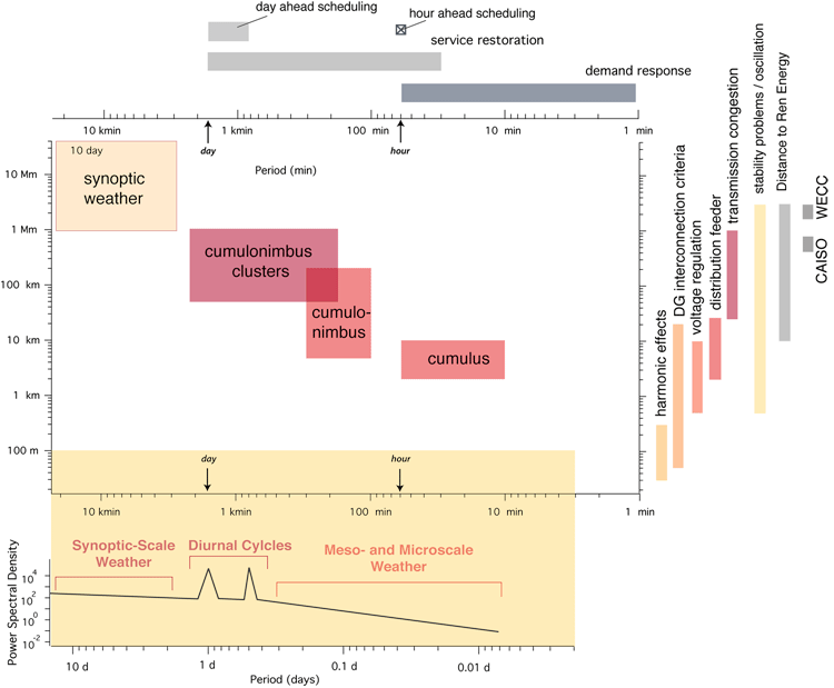
Ok, so after digging into Dr. von Meier's paper on the grid, we should have noticed a few things. First, renewables in CA are continuing to grow as a contributing portion of electricity generation. Second, the power grid linked with CA (the Western Interconnection) will have to accommodate the new sources of power just as the grid has to accommodate new loads (sources of demand). Before renewables, we had baseload power mainly from coal, nuclear, and hydroelectric, and everything was pretty smooth on the generation side of the equation. But now, wind and solar power are pushing in with "intermittent power."

In essence, renewable and distributed resources introduce spatial and temporal constraints on resource availability: we cannot always have the resources where we want them, when we want them.

-A. von Meier (2011)

This is a really neat paper, in that it points out the orders of magnitude of challenges that the markets and grid operators have to deal with on a regular basis, both spatially and temporally! And yes, you might also note that those scales were incorporated into Figure 5.10 of the SECS textbook for the Fujita relation of meteorological phenomena in space and time. You can compare the units in the von Meier paper with the table and graphic below.

We just learned that large portions of the electricity grid can be managed by an Independent System Operator (ISO, or RTO), where demand on the grid is managed through markets. That is great, but the grid also has problems that accumulate anyway, which need to be dynamically adapted to by the utilities or the clients. In our main reading, we see all the different systems elements that need to be coordinated in our power grids. These are amazingly complicated systems that are then perturbed by pesky things like weather.

Coordination in Time:

• Power Systems Management and Markets: Regulatory and technological parameters occur over time spans from years to days, to less than 1 minute (>6 orders of temporal magnitude). Pay special attention to Day Ahead Scheduling and Hour Ahead Scheduling while reading about markets.

Coordination in Space:

• Regional Power Grid Behaviors: Power responses, natural stability problems within the grid, transmission congestion, and regulatory scopes can happen over distances from thousands of kilometers down to tens of meters (>5 orders of spatial magnitude).

The Weather: yep, complicated too...

The weather systems that we deal with have their own orders of magnitude in time and space. Let's compare the time and space for weather phenomena in the following graphic. We saw this image in Lesson 3; but now, we can see that those time and space scales above actually fit with the scales right here, described by Ted Fujita. Notice the line that trends through the data of clouds (which are the nemeses of solar energy...). From a fit of $17\ m/s$, we have a quick conversion tool to flip between characteristic time scales and characteristic distance scales! Just remember $17\ m/s$ as the FRYB relation (Fujita-Rayl-Young-Brownson), and how to convert time from hours to seconds (3600 seconds in an hour), or kilometers to meters (you don't need that conversion, do you?).

Figure 8.2 Logarithmic scales of weather patterns that link spatial scales to time scales. The peaks for "diurnal cycles" are not from weather, but are rather from harmonics in transforming the diurnal behavior of day-night across a year into periods or frequencies. By inspection of the phenomena on Earth, we can identify an average advection rate of 17 meters per second, which becomes our conversion tool.

Credit: Jeffrey R. S. Brownson © Penn State University is licensed under CC BY-NC-SA 4.0