
Reading Review
SECS, Chapter 5: Meteorology, "Robot Monkey Does Space-Time" section
When we look at clouds, think of how they float by us without really changing in form all that much. Kind of like train cars passing by on the railroad, only much slower. We can use this to connect space and time (or frequency) in a useful way for solar resource assessment.Clouds (and weather fronts) occur on multiple scales of space and time. These scales contribute to the concept of solar fingerprints or climate regimes. In our reading, we learn about Sir Geoffrey I. Taylor and his work on turbulence theory. Clouds lead to intermittent solar conditions (POA and DNI irradiance) that, in turn, affect our solar energy conversion technologies, such as PV and building systems.
The intermittent variation of clouds as they affect the solar resource is crucial when solar is deployed as a large-scale farm, or as a large community of decentralized PV arrays on buildings. Variable peaks and valleys of electrical power can be detrimental (costly) to utilities if there are no other ways to store or shave variation on the grid. Now, storage solutions are emerging slowly in research, but right now we need to address the intermittency problem by better understanding the drivers and the basic science underneath those drivers.
Taylor's Hypothesis:
A series of changes in time at a fixed place is due to the passage of an unchanging spatial pattern over that locale. That is, when observing a cloud or thunderstorm passing overhead, the clouds of the thunderstorm floating by are effectively "unchanging spatial patterns" (big blocks of cloud). Put another way, the lateral change in the cloud conditions across regions of the meteorological event (e.g., cloud-sky-cloud-sky-cloud) can be directly connected locally with a variation in irradiance measurement over time (e.g., a periodic measure of dark-bright-dark-bright-dark).
Taylor’s hypothesis states that events that change in time for a fixed place are due to the flow or passage of unchanging spatial patterns over a locale. This is like observing a thunderstorm passing by directly overhead and making the connection to the rate of the clouds advecting with the thunderstorm. Taylor's hypothesis from the 1930s allows us to flip from the Eulerian frame of reference (time sequences) to the Lagrangian frame of reference (spatial changes).
The Eulerian frame of reference: When an observer is stuck in one place, only watching the changing phenomena as it passes by.
The Langrangian frame of reference: When the observer moves with the meteorological phenomena instead of remaining fixed. Imagine a flying carpet floating along with a cumulus cloud moving from one county to the next.
Hence, all scales of time (or frequency) are also spatial scales! Taylor's Hypothesis holds so long as the advective wind speed is much greater than the timescale of the evolving meteorological event being investigated, as is often the case. When you have a lazy cloud day, where the clouds are changing form faster than they move, the time-space connection doesn't hold anymore.
Connecting Scales of Space with Time
By using spatio-temporal scales of cloud features established by Ted Fujita, we can estimate an average translation (advection) speed of 17 m/s for meteorological phenomena. We can then convert the spatial scales of variability into a relevant timescale. Spatial scales associated with power transmission congestion are distances of 25-1000 km. These distances are relevant for meteorological phenomena within time scales on the order of 25 seconds to 16 hours.
Cumulus 2-5 km, which means 10-100 minutes.
Cumulonimbus (including anvil) 10-200 km, which means 1-5 hours.
Cumulonimbus cluster (including merged anvils) 50-1000 km, which means 3-36 hours.
Synoptic (including cyclone waves, short and long Rossby waves) 1000-40000 km, which means 2-15+ days.
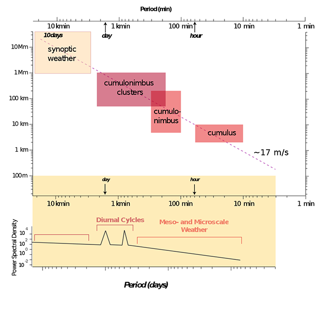
If we plot all of these phenomena and draw a line down the middle, we have a really rough estimate of the average advection rate of meteorological phenomena on Earth. Here, we have represented that rate in three different unit scales:
- 17 m/s [easy to remember this one, 17 is a prime number] or
- 1 km/min
- 61 km/hour (or 1470 km/day)
- 38 miles/hour (or 913 miles/day)
As such, we can connect Synoptic, Mesoscale, and Microscale meteorological phenomena between spatial and temporal scales!
General Scales of Meteorology in Space and Time:
Synoptic Weather: This is weather on the scale of 1000+ km in distance, and (given advection of ~17 m/s) seasonal timescales of 2-15+ days.
Mesoscale Weather: This is weather phenomena, including solar condition, on the scale of 100-1000 km distances, and time scales less than one day (hours).
Microscale Weather: This is variable weather phenomena on the scale of 10-100 km distances, and time scales of minutes to seconds.
Taylor’s Hypothesis “works” when the air in the sky moves significantly faster (advection: wind speeds) than the evolution time of a cloud or a thunderstorm of clouds. So, this approximation breaks down for those days when the cumulus clouds just "hang" in the sky all day.