Course Outline
Lesson 1 - The Historical Context of Solar Energy Valued in Society
1.0 Overview
Overview
Welcome to Lesson 1! Here we start talking about solar energy and the value that societies derive from solar energy options, both past and present. Many of us who are extremely interested in solar energy have yet to learn about the deep, deep roots that the solar field has established over and over again in societies across the world. Additionally, we hear about amazing new developments in solar in the media, events that seem to be happening weekly (and sometimes daily)! We would like to generate a sense for why solar energy applications are growing now, why they did grow and sometimes bust in the past, and what we might expect in the future.
We will use examples from reading, images, and your own experience to explore the differences between:
- Solar Resource (light from the sun),
- Solar Energy Conversion Systems as designed technologies, and
- Solar Goods and Services delivered by the combination of 1 and 2 (for example, electricity as 'solar good' and shade as 'solar service').
This lesson will also explore some historical aspects of the solar field, where societies have found fuels (geofuels such as coal, petroleum products, natural gas, and the biofuels such as wood and manure) more challenging to access due to various constraints. We will see that, in fact, an inability to access fuels is often the driving force for solar development. In contrast, when access to fuels is unconstrained, we find that solar development tends to slow or cease in society. In this lesson, we will also see how emerging solar industries correlate with global shifts in perspective regarding anthropogenic global warming, sustainability, and energy security. Frameworks will be explored for policy and entrepreneurial responses to these new perspectives.
1.1 Learning Outcomes
Learning Objectives
By the end of this lesson, you should be able to:
- Discriminate between (1) Solar Resource, (2) Solar Energy Conversion Systems, and (3) Solar Goods and Services;
- Explain the goal of solar design in terms of locale, stakeholders/clients, and solar utility;
- Connect the historical and modern contexts for solar energy growth/recession to stakeholder preference, fuel constraints, and solar rights/access.
What is due for Lesson 1?
This lesson will take us one week to complete. Please refer to the Canvas Calendar for specific timeframes and due dates - those can vary from semester to semester. Specific directions for the assignments below can be found further within this lesson.
| Required Reading: |
J.R. Brownson, Solar Energy Conversion Systems (SECS), Chapter 2 - "Context and Philosophy of Design" J. Perlin, "Let It Shine: The 6000-Year Story of Solar Energy", Chapters 2, 3, and 6. (These books can be accessed online via Library Resources tab in Canvas or by search of Penn State's Library. You must be a Penn State student to access this text via the E-Reserves). |
|---|---|
| To Do: |
Learning Activity: Identifying the Components of SECSs Yellowdig Discussion: Historical Development of Energy Resources Download NREL's System Advisor Model (SAM) Engage in all Try-This and Self-check activities (not graded) |
| Topic(s): | Energy constraint, value of solar energy, history of developing solar energy |
Questions?
If you have any questions, please post them to the Lesson 1 General Questions and Comments discussion in Yellowdig. I will check that forum regularly to respond. Feel free to go through the comments and post your own responses if you are able to help out a classmate.
1.2 History of Human Energy Supply and Demand
Reading Assignment - Energy Primer
Please review the Energy Explained [1] portion of the USA Dept. of Energy's Energy Information Administration [2] website.
When you are reading, I want you to focus on Forms of energy, Sources of energy, and Supply (production) vs. Demand (consumption) of energy. These four terms are simple but very specific. One thing that you can use to remember them: energy is neither created nor destroyed, but can be transformed from one form to another, and we call our sources of energy resources. The economics of energy is also directly discussed in terms of supply and demand.
Energy Demand in USA Society
We believe the global demand for energy in its various forms will keep rising, spurred on by an expected increase in population and industrialization of many developing countries. Policy makers, entrepreneurs, and scientists will be faced with serious questions on how to produce and deliver required energy to consumers. But focusing in on the USA, how does a country use energy where local population growth is smaller and energy use has been outsourced to other developing nations?

Bottom of chart displays dates from approximately 1775 to nearly 2010, marked in increments of 10 years. The left side of chart displays Energy consumed in Quadrillion BTUs, marked in increments of 5 Quadrillion BTUs. Six types of fuel are displayed on the chart: Wood, Coal, Petroleum, Natural Gas, Nuclear, and Hydro.
Wood begins at a little above 0 Quadrillion BTUs in 1775 and stays low, rising to only about 4 at its peak in about 1870.
Coal begins at a little above 0 Quadrillion BTUs in about 1850, becomes the primary fuel source from about 1883 -1950, rising to a height of about 17 Quadrillion BTUs in the 1920s and 1940s (with a dip in the 1930s), suffers another dip from about 1950-1960 (during which time petroleum and natural gas were gaining great ascendency), then rises again to about 22 Quadrillion BTUs by the early 2000s. Coal begins dipping again as the chart ends near 2010.
Petroleum begins at about 1 Quadrillion BTUs in about 1900 and starts to rise sharply by about 1917. By 1950, it equals coal at about 12 -13 Quadrillion BTUs. Petroleum continues to rise sharply, reaching a peak of close to 40 Quadrillion BTUs in the early 2000s. Petroleum begins dipping again before the chart ends near 2010.
Natural gas is close to 1 Quadrillion BTUs in about 1920. Its usage rises to about 23 Quadrillion BTUs by about 1970 before dipping in the 1970s, then rising again to about 23 Quadrillion BTUs by the end of the chart.
Nuclear begins at just above 0 Quadrillion BTUs a little before 1950, stays steady until close to 1970, then begins rising slowly to a peak of about 7 Quadrillion BTUs by the end of the chart.
Hydro begins at just above 0 Quadrillion BTUs in 1775 and stays low, rising to about 4 Quadrillion BTUs at its peak in the late 1990s.
Trends and milestones in the past few centuries
1880 to 1920:
- Farming work displaced by machines (industry).
- USA urban population grows from 28% to 50%.
1883:
- Fossil fuel combustion (coal) equal to biofuel combustion (wood).
1950-1980 (Post WWII):
- US urban population growth slows.
- Cars and highways lead people to the suburbs.
- Manufacturing decreases (outsourcing energy).
2010:
- Renewable energy surpasses nuclear power: exponential growth of the renewable industry kicks in hard!
- Wind surfaces as a large renewable energy player.
- Solar emerging: Decentralized solar power is rapidly expanding on rooftops ("behind the meter")
2010-2020:
- Emergence of 100% renewable cities and communities – USA: Rock Port, MO (2008); Greensburg, KS (2013); Burlington, VT (2014); Kodiak Island, AS (2014); Aspen, CO (2015); Georgetown, TX (2018). More than 40 cities globally. (CleanChoice Energy [4], 2024)
2019:
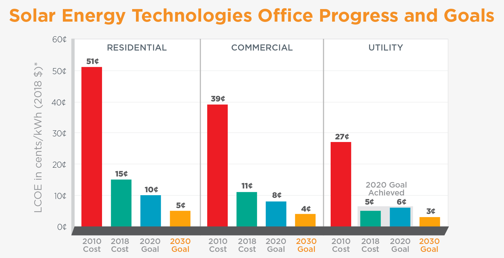
- Solar energy system costs hit historic lows, falling ~70% over the 2010-2020 decade, to become economically competitive with other energy sources.
- Significant growth of solar installed capacity: total new electric capacity increased from 4% in 2010 to 40% in 2018 in the USA.
2020:
- Globally, renewable sources demonstrated the fastest growth over the past two decades reaching over 11% contribution to the global energy mix.
Year Fossil fuels Wood biomass nuclear renewables 2000 77.3% 10.2% 5.9% 6.6% 2020 78.0% 6.7% 4.0% 11.2% Source: World Economic Forum [5], 2022
The Big Picture
Click here [6] to see the larger version of this chart.
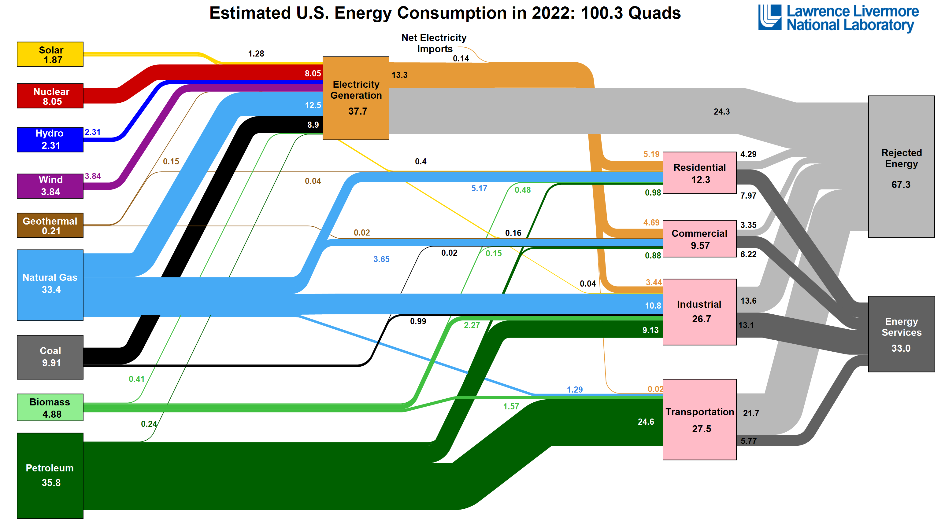
This annual energy flow chart shows the total energy generated by different sources and consumed by different sectors. The units used here are quadrillions of Btu’s (“quads” for short) indicate massive amounts of energy used at the national scale.
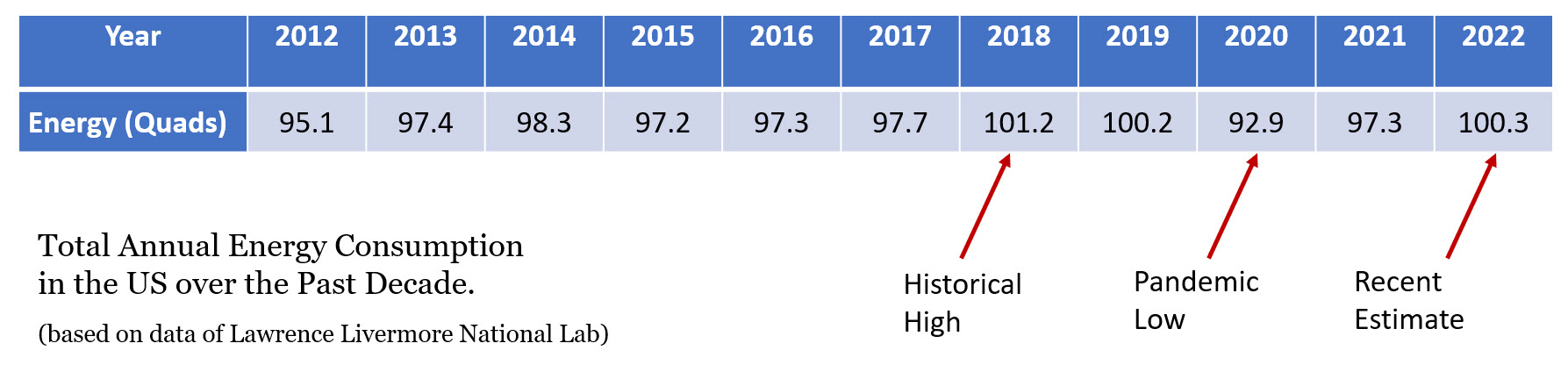
The total estimated energy consumption in the US in 2022 is around 100 Quads, and this number is on the upper end of the typical consumption bracket:
The contribution of solar energy has not yet approached the magnitude of traditional fossil fuel sources in the US, however its contribution to the renewable share of the electricity generation is actually substantial.
Let’s crunch some numbers:
National Electricity Mix
Total renewable energy share (including solar, wind, hydro, biomass, and geothermal) in the electricity sector sums up to 7.9 Quads (21%), which is comparable to 8 Quads (22%) for nuclear energy, 8.9 Quads (24%) for coal, and 12.5 Quads (33%) for natural gas. That is about 1/5 of the entire national electricity mix. If we look back at similar data for the year of 2012, renewables only accounted for 12% at that time.
What sources are fastest growing?
Comparing the data from the historical energy data from a decade ago (2012) and the most recent (2022), the fastest growing generation capacities are solar, wind, and natural gas. Nuclear remained steady, hydropower and geothermal showed small decline, biomass – small increase, and coal was on significant decline over these ten years.
Summarizing the trends:
| Sector | Growth from 2012 to 2020 |
|---|---|
| Solar | + 698% |
| Wind | +182% |
| Natural Gas | +28% |
| Biomass | +13% |
| Nuclear | 0% |
| Geothermal | - 7.5% |
| Hydropower | - 14% |
| Coal | - 43% |
Look up the historical versions of energy flow charts here [7].
By a big margin, solar has been the fastest growing source (almost 7-times growth!) in the national energy industry. The impacts were primarily seen in the residential and commercial sectors, which in addition to the grid may benefit from the distributed generation options (small-scale and off-grid installations).
Projections
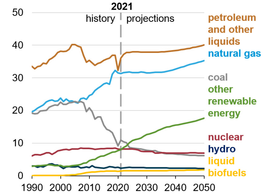
Projections shown in this plot are based on the analysis of energy markets by EIA: “we project that renewable energy will be the fastest-growing U.S. energy source through 2050. Policies at the state and federal levels continue to provide incentives for significant investment in renewable resources for electricity generation and transportation fuels. New technologies continue to lower the cost to install wind and solar generation, further increasing their competitiveness in the electricity market, even as the policy effects we assume level out over time.”
“We project that consumption of natural gas will keep growing as well, maintaining the second-largest market share overall. The expected growth in natural gas consumption is driven by expectations that natural gas prices will remain low compared with historical levels.” (EIA, AEO2022 [8])
Major Players
In the past century, society has been dependent on combustible products such as coal, natural gas, and petroleum products as the fuels of choice. While these energy sources are relatively cheap, they are not always available or located where we most need them, and they are non-renewable. In addition to this, there are real concerns about the effects burning these products could have on human health and safety as well as large impacts on the environment in general. The following are geofuels (resources from the Earth that are non-renewable).
- Coal (fossil fuel)
- Petroleum derivatives (fossil fuel)
- Natural Gas (fossil fuel)
- Nuclear (fissile fuel)
Nuclear energy is an additional geofuel that does not have a major CO2 impact and is a major resource in countries like France. However, it has a strong "yuck factor" for the majority of society in Germany and the USA. It has the additional challenge of undesirable proliferation of fissile material for arms use. Again, there are numerous countries including the USA that make use of nuclear power for low-CO2 energy, but infrequent, high-visibility events such as Three-Mile Island, Chernobyl, and Fukashima Daiichi continue to influence popular will to invest and develop the resource.
Renewable energy sources provide a suitable alternative to using fossil fuel combustion (which generates CO2) to meet our energy needs. The well-planned use of renewable energy sources such as solar energy must form a part of the portfolio of energy sources. There are numerous real challenges for renewables like solar, such as intermittency and diurnal cycles (night-day), as well as the ability to identify economic opportunities, which is why we are putting a lot of effort into understanding the solar resource and the related economics in this course.
Energy production and CO2 production—link to population
The following link uses Gapminder World to show the increases in cumulative CO2 production through time associated with population growth. Click on the link and press "Play" in the bottom left of the diagram:
You can explore this tool later and create your own plots with respect to time. For example, if you were to plot energy production (Supply) or use (Demand) you would see the same trend, or if you were to plot cumulative CO2 (log) vs. total energy production (log), they would show a rough linear correlation. But, for now, I want you to see where there are links between population, energy production, and CO2 production. Why is the USA more or less stable in its CO2 production?
1.3 Discussion Activity
Yellowdig!
This semester we are adopting a new platform for class discussions – Yellowdig! If you have only participated in the Canvas discussions so far, this may feel a little different. My hope is that this tool will help us make the discussions more engaging while maintaining the breadth and depth of learning we hope for. Please refer to the course orientation page that explains the steps to establish your Yellowdig account and set yourself up for participation.
Already have the Yellowdig account? – Then go to Canvas course menu, and click on “Yellowdig” link on the left to enter the conversation space.
Lesson 1 Discussion: History of Energy Resources
For this first week of the class, I would like you to engage in conversations about the historical development of energy resources in your area – solar and beyond! Here are some guiding questions that will set you up and help you create good posts and initiate productive discussions:
- How far back in time can you find historic energy information for your locale?
- What are the traditional sources of energy and fuels (geofuels) your region relied on in the past?
- What is the history of solar energy use in your area (not limited to solar panels – think broader!) for heating, cooking, power etc.
- From your own perspective, how good is the solar resource where you live and what it may mean for the economy of your locale?
Some of these questions will require you to dig in a bit and research outside of this class content. Expect that it will take some time to find good, resourced information.
Tagging
Yellowdig Tip: When you create a post in the Yellowdig discussion space, you are required to choose a topic tag. For Lesson 1 discussions, use either (or both) of these tags:
You can create a single post or split it into two different topics – whatever feels best for you!
Importance of interaction
When it comes to Yellowdig, your posts, comments, replies, questions and answers – all these may add points to your yellowdig score, so don’t hold back! In order for these activities to work best for your learning, you need to participate frequently, keep up with conversations going and take opportunities to interact with your peers. Sometimes spontaneous conversations sparkled over a single fact mentioned bring more value than initial content.
Grading
Yellowdig discussions will account for 15% of the total grade in the course. Your posting and interactions will contribute to your weekly participation score (1000 pts.). After each week, all the Yellowdig points you earned will be transferred to Canvas and added to the your cumulative participation grade. Check the Orientation Yellowdig page for more details on the points earning rules – how many you get for starting a conversation, posting a comment, or attracting traffic on your post.
Notifications
Be sure to set notification preferences in Yellowdig if you’d like to receive emails about someone posting or replying to your post. That will allow you not to miss important action as you go through the week.
Deadline
I encourage you to create your posts in the middle of the study week (Sunday) and not to wait until the end of the lesson. That will allow others to respond in a timely manner. Each conversation will stay open after the lesson is done, but it will be harder to earn a high score with your work once everyone moved on to the next lesson. Note that point earning window for each lesson is limited to one week.
1.4 Solar: the Response to Energy Constraints
Reading Assignment
- J.R. Brownson, SECS, Chapter 2 - "Context and Philosophy of Design".
- K. Butti and J. Perlin, "A Golden Thread: 2500 Years of Solar Architecture and Technology", Chapters 1, 2, and 5
(Electronic course reserves, or "e-Reserves," are articles and book chapters that are available online through the University Libraries. Access this lesson's reading by going to Library Resources in Canvas and selecting E-Reserves for EME 810)
These two readings will provide our introductory perspective on solar energy in society. I want you to think about the impact of perception in society. Some of the "constraints" in society are real, physical limits to fuel access, while others are much more subtle--but both have a similar response to induce people to adopt alternative energy strategies.Energy Constraint Response
We can observe that popular perception of solar energy is strongly influenced by access to inexpensive fuels. In periods when fuels were effectively accessible, inexpensive, and unconstrained, a light-induced energy transfer (for sensible or latent heat change or for electricity generation) is usually perceived as diffuse and insufficient for performing work. However, for periods in history where fuels have become constrained (e.g., inaccessible due to high cost or high risk), innovation has turned to solar technology solutions. In such cases, the use of light-induced energy transfer is perceived as ubiquitous, and ample for performing work.
Evidence of such fuel constraints is observed as far back as the fifth century BC. During this period, the Greeks faced severe shortages of wood fuel. Archeological remains demonstrate that home designs evolved such that all houses could draw maximal utility from the Sun's warmth in winter months. It is interesting that famous Greek individuals commented on this solar design of homes. Aristotle has commented that home builders would shelter the north side of a home to keep out the cold winter winds. Socrates also lived in a home heated by the sun, and observed, "In houses that look toward the south, the sun penetrates the portico in winter" keeping the space warm (Note: a portico is just an older term for a porch). The Greek playwright Aeschylus further noted that only primitive cultures "lacked knowledge of houses turned to face the winter sun, dwelling beneath the ground like swarming ants in sunless caves." How primitive have we been these years without solar designed homes?
The Sun as a large stock for Renewable Energy Resources
A renewable resource has a rate of withdrawal (a flow) from the stock that does not exceed the rate of resource replenishment.
Sun: pretty big stock for wind and solar.
The sun provides energy in the form of radiation. Solar radiation is the most important natural energy resource available to us because it drives all environmental processes acting at the earth's surface. It drives the earth's rain cycle, which powers modern hydroelectric generators, and large-scale atmospheric circulations which provide the winds that have powered windmills for centuries. The sun doesn't warm the air, because the sky is largely transparent. The sun warms the ground which then warms the air. We will show how solar energy conversion devices often take advantage of the solar-thermal connection. In fact, we can often take advantage of air masses contained by walls, trees, or hills to trap and store thermal energy from the sun.
Solar energy technologies convert solar irradiance (sunlight) into forms of energy found useful to society. Historical and current developments in solar technology often coincide with specific economic or fuel constraints. As we observe from our reading assignment, technologies using solar energy conversion have been developing for a long time. Solar and wind power are among the options providing a low or non-CO2 associated energy source for electricity production. Solar energy is also a natural part of heat production in buildings or solar thermal plants. This section will review the value of solar energy from a historical context while also discussing the origins of using solar energy and the present-day development of the solar energy industry.
Controlling Home Heating: Passive Solar
Below is a link to a video of the Ryoan-ji Zen temple in Japan. Look to the left of the marker at the white field just to the south of the brown roof (you will need to zoom in a few times first). This is the famous rock garden of the temple. The white field reflects light into the adjoining room to the north, and the walls surrounding the field keeps cool air inside the area. As a side note, the icon you see on the building is a map symbol for a Buddhist temple.
All right. So, what you're looking at here is a map view in Japan of a Buddhist temple called Ryoanji. It's just outside of Kyoto. And what we want to really focus on here is that this is an example of using the solar resource in a way that is old actually, but very traditional and has a really high value to a group of people. So, this is actually a temple.
And if I go in here, I should be able to show you that the—nope, I cannot.
There we go. I should be able to show you that in this map, we've got here a direction that is South. So, we're in the Northern Hemisphere. This the South. That means that this whole white space is a great area for reflecting the sun's light. And it will actually reflect the sun's light into the space just to the North. That space is actually going to be an area for working, writing, copying down what we would call sutras.
And it's very interesting because you have a white surface that is directing visible light into that space. And in doing so, you're actually avoiding using fuel to provide the lighting. That actually improves air quality. And you are avoiding the cost of that fuel in the process of doing this.
Now, if we look at the image of Ryoanji here, here's that rock garden. So, close up, you're starting to see something that you recognize, at least from popular culture, which are these calming Zen rock gardens.
The interesting thing here is that the rock garden itself is very functional. Again, it is going to be bouncing light into the space where people are working so they get much better light. In addition, think about it. White objects do not absorb light. So, by the very nature, they're reflecting light. So, you have an area that is not going to be warmed up during the day. And in fact, this is a very bright area. And it's going to remain somewhat cool. You're going to create a microclimate of cool air.
And then you have walls. And the walls are there to contain that cool, stored air. If the walls were not there, the air would just sink and flow away from the cool area. So, you're containing and storing this cool thermal energy. That, in addition, is connected to the space that we're seeing right in here. It's connected to this space. There are open doors through here, so you got cool air coming in. And you're seeing that this is one way to use solar energy for some very high-functional use.
And if we go again back to the Zen rock garden-- this is the same garden. You notice that there are rake imprints. And there's this classic idea of Zen monks raking this in a meditative process. We even sell small sandboxes with little miniature rocks and rakes to simulate a rock garden. But the actual value of this rock garden is very functional.
And so, when you rake those rocks, what you're actually doing is removing leaves. You're removing any growing moss or lichens on those rocks. You're maintaining the brilliance of those rocks as a good reflector. And so the process of raking is actually again, functional to maintaining your solar reflection device, which you're seeing here at Ryoanji.
If solar energy is this important, and the Greeks in the fifth century B.C already recognized this, you may ask why solar energy applications are not more prevalent than they are at the moment? While there is no simple answer to this, there are still many obstacles that lie in the way of its widespread adoption. The future of solar power development will depend on how we deal with constraints such as scientific and technological problems, marketing and financial limitations, and political actions and agreements that favor other energy sources.
For more information on solar home design (also termed "passive solar"), see the California Solar Center: Passive Solar [12].
Hot Air and Water
Horace de Saussure was a Swiss naturalist of note to the history of solar development in the 18th century. He began to explore the role of a glass cover on a confined space like a box or a room. In the 1760s, de Saussure observed the following: "It is a known fact and a fact that has probably been known for a long time, that a room, a carriage, or any other place is hotter when the rays of the sun pass through glass." To find out how effectively a glass cover works to trap solar gains, de Saussure constructed a large flat pine box that was insulated inside, with a glass cover on top. Inside the box, he placed smaller boxes. When the flat cavity-cover absorber was exposed to the sun (no concentration), the internal box heated to 109 °C (228 °F), which is 9 degrees higher than the boiling point of water.
Cross-section of Langley's hot box (solar thermal box with two glass covers and a thermometer on the inside), which was similar to de Saussure's later models. A thermometer penetrating the walls at the right was used to measure the air temperature inside the inner box.
Functionally, the clear glass allows shortwave irradiance to transmit through and be absorbed by the dark interior of the box. In addition, the glass cover prevents the warm air from escaping. This is a classic flat plate cover-absorber system. The hot box that de Saussure began with later became a prototype for flat plate solar hot water panels, providing hot water to millions since 1892. The hot box also led to the development of modern solar cookers. For more information on solar thermal design, visit the following links:
- Solar Thermal Energy for Homes [14]
- Horace de Saussure and his Hot Boxes of the 1700s [13]
- How Solar Cooking Works [15]
Photovoltaics
While photovoltaic materials were explored in the 1860s, tied to research in transatlantic telegraph cables (using selenium; by electrician Willoughby Smith), they did not emerge into the larger market until nearly 100 years later. Photovoltaics using silicon material were introduced to the commercial world during the early 1950s by three lead scientists at Bell Laboratories: Calvin Fuller (a chemist), Gerald Pearson (a physicist and materials experimentalist), and Darryl Chapin (a device engineer). The development of a silicon-based PV cell led to applications in space and telecommunications first, followed by applications for the petroleum industry (for anti-corrosion in wells).
PV has proved itself as a standard technology for decades. All of today's satellite communications are powered by photovoltaics, starting with the Vanguard 1 [19] (which had no "off" switch, and so continued to transmit long after it needed to). So, be thankful, we would not even have a modern society without the advent of PV!
For more information on photovoltaics: check out the following sources:
- Supplemental Book and reference: From Space to Earth: the story of solar electricity. by John Perlin. ISBN 0-937948-14-4, available from the Penn State Libraries.
- The first PV device was made by 19-year-old André Becquerel in his father's laboratory, in 1939, Wikipedia article on A.E. Becquerel [20]
- PVEducation.org [21]
- California Solar Center: Photovoltaics [22]
Review
Constraints have included wood shortages in Greece and Rome in early centuries BCE, shortages of trees and fuel in the Chaco civilizations of the Anasazi peoples of North America, coal reserve constraints in 19th century France, and fuel access constraints in rural California before the 1920s. We have recently (the past decades) entered into a new period of constrained fuel consumption due to climate forcing effects from anthropogenic greenhouse gases (associated with fuel combustion, agriculture, and high energy demand), as well as increased risk in supply chains for fuels (the quest for energy independence).
1.5 What is a Solar Energy Conversion System?
Reading Assignment
- J.R. Brownson, Solar Energy Conversion Systems (SECS), Chapter 12 - "Systems Logic of Devices: Patterns"
We are jumping far, far ahead to see where we can take the concept of a Solar Energy Conversion System in society. The text in Chapter 12 complements your reading of Ch 2 and goes in depth to identify the different technological patterns in solar energy conversion systems. I think you will find the content relevant in the broad sense of designing systems, and that it will engage your creative processes for the future project at the end of the course.
Think about the way in which so many of our technologies and biologies are in fact "solar energy conversion systems," with some or all components of a functional aperture, receiver, distribution mechanism, storage, and control mechanism. What may be even more interesting is when you start to identify collections of different SECSs in the same space.
An important context of the approach to solar energy is understanding what a system is. We define a system as a collection of elements that are connected together via weak or strong network relations and that have a pattern or structure that yields an emergent set of behaviors. We are concerned, in this course, with environmental systems, each with boundaries that describe the system and its surroundings.
A Solar Energy Conversion System (SECS), as the name implies, is a system that converts the energy from the solar resource into work found useful by society. This system has the potential to be deployed as an ecosystems technology or an environmental technology, meaning the energy system interacts in a constructive way with the patterns of nature. As a process, solar energy conversion calls upon designers and engineers to include all the elements essential for the proper functioning of a conversion system. These include the Sun, the Earth and the applied technological system (for example solar thermal or solar photovoltaic) in question. These systems call upon researchers to simultaneously assess scales of solar resource supply and use, systems design, distribution needs, predictive economic models for the fluctuating solar resource, and storage plans to address transient cycles.
Collector Basics
We have reviewed the basic system concept that can be used to design solar energy conversion applications, and more detailed and thorough information will be presented in a future lesson. At this point, we move on to the nature and composition of SECS on the Earth side (incident surfaces).
A Solar Energy Conversion System consists of the following elements:
- Aperture (the opening to allow light in, and at the same time constrain the solar flux into the system);
- Receiver (the opaque absorber that converts the sun to other forms of energy, the active element that is responsible for energy conversion);
- Storage (sometimes there will be a designed or naturally present storage mechanism, as sunlight is intermittent);
- Distribution Mechanism (internal to the system, responsible for energy delivery);
- Control Mechanisms (which helps adapt the conversion process to the intermittent/seasonal changes and user needs).
The next section of this lesson provides you with an exercise to identify these elements in several different solar energy conversion systems functioning in diverse settings.
1.6 Lesson 1 Learning Activity
Activity: Identifying the Components of Solar Energy Conversion Systems
Based on the reading in the previous page of the lesson, we understand that almost everything exposed on the Earth's surface can be described in terms of a solar energy conversion system. Some systems are capable of producing more useful work than others, and there are both technologically designed and natural systems. We will use this activity to explore this concept and to identify various SECSs embedded in society. Some will be obvious in the context of this class, while others will require a more nuanced view or a creative perspective.
Take a look at each of the following five images, and thoughtfully locate as many SECSs as you can in each one. Now, try to identify and list the functional components (aperture, receiver, storage, distribution, mechanism, and control mechanism) for each of these SECSs and think about how they work. Please write a short paragraph for each image that identifies all of the SECS’s as well as an explanation of how each one serves as a component. It may even be possible that some of the systems are themselves components of a larger system, in which case you will need to dial out your perspective to a larger system.
Do your best to explore and be creative rather than looking for all the "right" answers.
 [23]
[23]  [24]
[24]  [25]
[25]  [26]
[26]  [27]
[27]
Submission
Please fill in the "matrix" (Excel spreadsheet template provided) based on the results of your analysis. You are also welcome to provide any additional discussion on the systems you observe in the images. Submit your work into “Lesson 1 Learning Activity Dropbox” in Canvas.
Grading Criteria
This activity is graded out of 20 points. Each image is worth 4 points, 2 points for identification of the components and 2 points for your explanation.
Deadline
See the Canvas calendar for specific due dates.
1.7 Frameworks for Including SECS
Reading Assignment
- J.R. Brownson, SECS, Chapter 2 - "Context and Philosophy of Design".
Come back to review this Chapter specifically focusing on the Frameworks sections.
The last activity emphasized the way that SECS can "work" as a functional system. Now, I would like you to read and reflect on the broader concept of "design" as pattern with a purpose in society and the environment. As you are reading, look into the ways that society has established frameworks for integrating solar goods and services into local solutions (which we will expand upon as "locale"). The following points are highlighted in the text.
- Solar as Lighting Aid
- Solar Rights and Access
- Solar Power Entrepreneurs
- Solar Ecosystems Services
In this section, we are going to be looking at some of the same pictures we saw in the Learning Activity, but from a different perspective. We will call the following case studies "frameworks," and investigate the value of solar energy conversion systems in different contexts. Consider the following frameworks as interpretations of valuing the solar resource and the resulting solar goods and services by society (in economic and sustainability terms): the same resource can be applied to different client needs, the way that we have set up legal ramifications to protect access and rights to the resource, the entrepreneurial/ecopreneurial spirit that is a part of SECS design and implementation, and the ecosystems services that surround our SECSs.
Solar as Lighting Aid
NPR Audio Article [28] (Transcript available on the website)
Many of us will come into the field of solar energy with a slightly biased view that the solar resource is useful for making electricity (a preferred solar good by many stakeholders) using photovoltaic technologies (the Solar Energy Conversion System of note in current society) or for making hot air or water (like a solar hot water panel, another SECS technology). However, we must be also aware of the use for daylighting. Daylight is as essential to human health as clean water and air. The variable intensity of daylight has been found to increase alertness within the office space (as opposed to constant light conditions with artificial lighting).
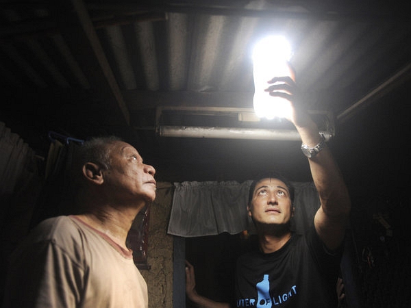
In the case of a Liter of Light (see link to NPR article, above), the ecopreneurial venture by this non-profit means using appropriate technology to deliver a high solar utility (again, meaning a preference to the set of goods and services from solar energy conversion systems) to their clients at accessible costs. The bottles are discarded 1 L plastic soda bottles, filled with water and a drop of bleach (to minimize algal growth or other microbes). The technology is the same as a "light pipe," or a fiber optic, using different indices of refraction between air, water, and plastic to create a phenomenon called total internal reflection. On boats, this type of light direction uses a centuries-old SECS technology called a deck prism [30].
Not only do these warm climate homes benefit from better lighting, they also avoid fuel costs for electricity (if available) and combustible fuels such as kerosene. Additionally, the solar bottle light pipes will improve indoor air quality by reducing fuel combustion inside.
Solar Rights and Access
While the solar resource from the sun is available at no cost to us, there are laws that may restrict the way we intend to use the sun for purposeful work. Designers will often call the accessible area for solar implementation the "solar envelope," but how do we maintain the legal rights to make use of or access our own solar envelope, and can we make sure that solar technologies can even be installed in our locale? Legal structures for solar energy is not a new concept. In ancient Rome and Greece, legal structures were set up in the form of easements, allocated government lands, and sometimes strict urban planning for orientation and elevation limitations on entire communities.
Solar rights define access to solar energy and hold significant economic consequences. They dictate whether a property owner can grow crops, illuminate his space without electricity, dry wet clothes, reap the health benefits of natural light, and perhaps most significantly in our modern era, operate solar collectors.
In the USA, we distinguish between solar rights and solar access.
- Solar rights give you the option to install a specific solar energy system within residential or commercial properties otherwise subject to private restrictions.
- On the other hand, solar access ensures that a structure receives sunlight across property lines without obstruction by neighboring objects, including trees.
- Examples of common private restrictions are bylaws that forbid PV on roofs, or clothing drying lines anywhere.
- Over 40 states have adopted solar access laws either in the form of a Solar Easement Provision or/and a Solar Rights Provision.
Solar Power Entrepreneurs
Entrepreneurs are generally great contributors to the commercialization of interesting and useful technology. The field of solar energy is no different. An important character in the development of SECSs is Frank Shuman, an eclectic inventor in the late 1800s. Shuman formed the Sun Power Company in 1910 and successfully harnessed solar power physics to generate steam pump power in Egypt in 1911.
New entrepreneurial ventures in solar are often also humanitarian and ecological in nature. SolarFire.org and Liter of Light are two examples.
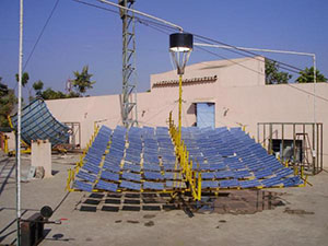
The Prometheus 100 solar concentration systems for steam generation can be seen in the image above. Mirrors (the aperture) are focusing shortwave light onto an upper central receiver (glowing bucket), where steam is produced. The steam is running a small steam generator pictured in the lower left of the image. The supply water is pumped in from the tube seen in the upper right. The entire system plans are available as open-source information, and can be machined with accessible local technologies and inexpensive materials. This system was installed in Rajkot, India.
Solar Ecosystems Services
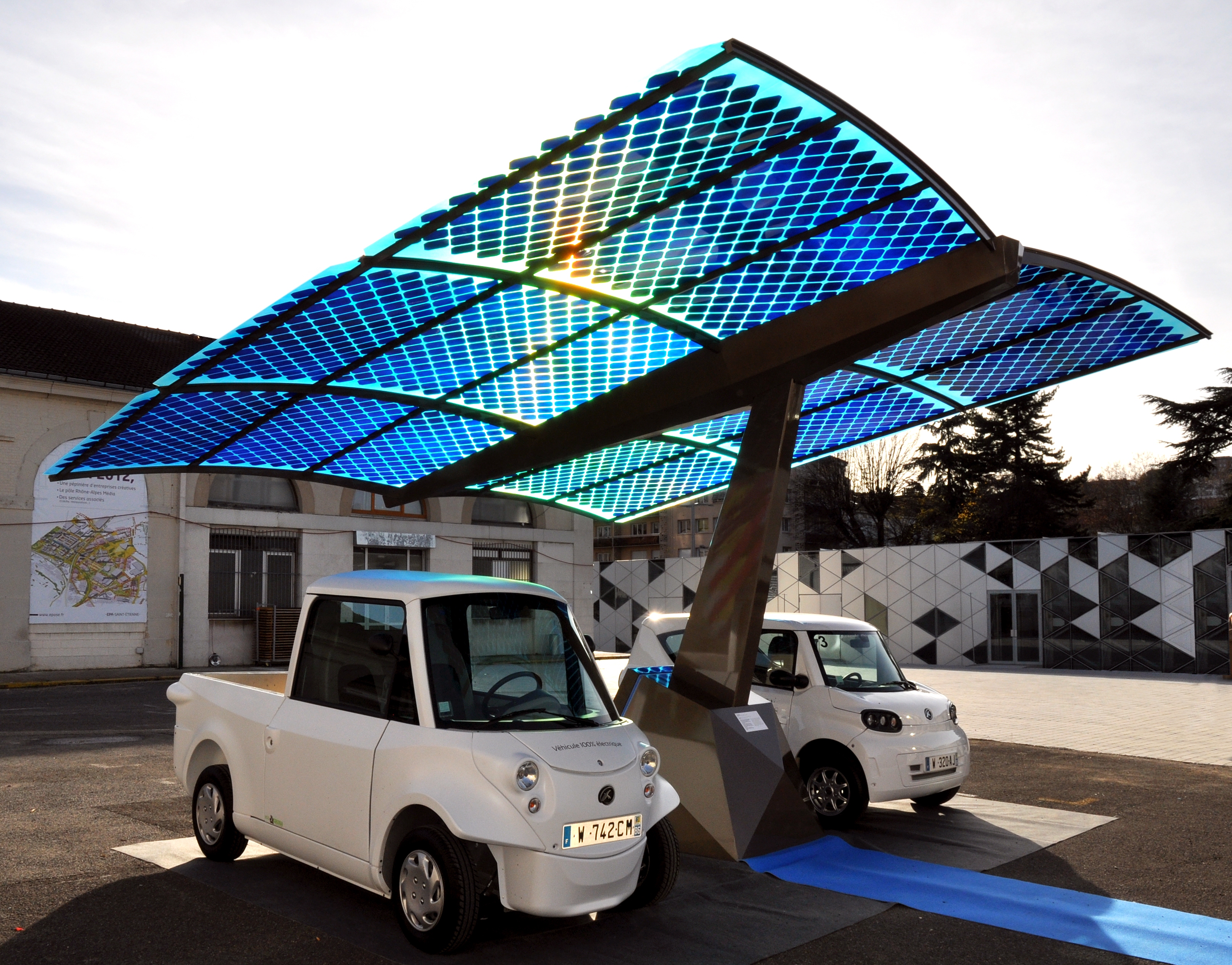
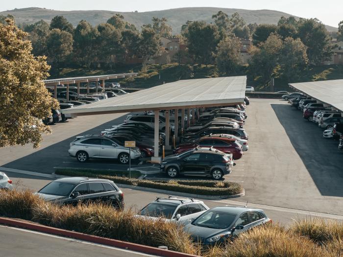
Any solar technology will have an impact on the ecosystem in which it is deployed. In addition, it could add ecosystems services to the area if designed with an awareness for landscape architecture and ecology. Presently, design teams discuss manners in which photovoltaic arrays can add desirable shading in addition to power generation (desirable shading would be considered a preferred solar service). One common method is to design and install a solar panel to also serve as a shading structure for cars in a parking lot.
- Supporting services or habitat
- Provisioning services
- Regulating services
- Cultural services
You may wish to read the short descriptions of the various services from The Economics of Ecosystems and Biodiversity (TEEB [35]) website. They have created a fairly concise list with descriptive sections that clearly identify valued processes that emerge from a resilient ecosystem. Remember: our technologies and our societies are always a functioning part of our ecosystems in the locale that we operate, even if it doesn't quite seem that way in our daily lives.
Supplemental reading
1.8 Introduction to SAM
Download System Adviser Model (SAM) Simulation Software
NREL's System Advisor Model (SAM) [37]will be a useful simulation tool for this class. You will be required to use it for some of lesson assignments and your project. So I would like you to take the time to download and try launching SAM on your computer this week.
The NREL website linked above also has a webinar video, which walks you through the key functions of SAM. Please feel free to watch it at your leisure.
Directions
- Create a User Account [38] and choose Photovoltaic as the Technology Focus at the bottom of the page.
- Follow the download and installation instructions.
NOTE: SAM is an Open Source project! The version of System Advisor Model as of the update of this page is SAM 2023.12.17 (and there will likely be newer versions each semester). It requires about 1 GB of disk space, and either Windows 10/8/7 or OS X 10.9 Intel or later. SAM is a 32-bit program that will run on both 32-bit and 64-bit operating systems. If you do not have one of these operating systems, you can browse their list of Legacy Versions as an alternative.
- Install and launch SAM on your computer. The very first time, you will need to enter your email and click the "Register" button. SAM will send you a code to use in the next entry for "Key". Paste it in and get rolling!
- Try to "Start a New Project" with Photovoltaic Detailed Model for a Distributed scenario. The defaults are pretty reasonable in SAM. If you've never tried something like SAM, don't worry. This is really just an exploration step, and you can't really break anything by opening a new project and running it. So, just explore a little and have some fun.
- If you successfully create a new project, you can browse through the system parameters and options on the left side menu. Check the defalt numbers. You will see that you can change the values in the white boxes, and numbers in the blue boxes will calculate automatically.
- Hit the big blue box in the lower left labeled SIMULATE > . The program will run a year's solar data and will output a heap of results. The output in the table is the summary of stats for the project, usually estimating 25 years of a solar project.
Deadline
There is no deliverable for this activity, but I strongly encourage you to take initial steps for installation and creating a project in SAM this week. Lesson 2 will give you some work to complete in SAM, so it will be useful to have it up and running.
Yellowdig Conversation
Feel free to share your thoughts, questions, and tips on the SAM software in the Yellowdig space. Use the topic "Starting with SAM" for your posts. This is not a required activity, but it can still boost your participation score for this week.
1.9 Summary and Final Content
Summary
We have just finished looking at the historical and modern contexts for valuing solar energy (and SECSs) in society. I wanted to put you in the frame of mind that solar energy as a valued resource is a flexible concept. The value expands with energy constraints and with positive health and safety implications; the value shrinks with the reduced costs of alternatives such as fuels. There are many different ways that society values the solar resource, however, and as a part of a design or engineering team (or part of a policy team), we should remain creative and persistent in trying to develop and expand SECS deployment into society.
You have made your first step toward the solar assessment project that we will present to our peers in Lesson 12 at the end of the course. I would like you to make sure that you have found the SAM (System Advisor Model) [39] website and downloaded the software onto your systems. Your future clients/stakeholders will be informed by your creative ability to present them with a valuable solar resource in their locale, one which also yields financial benefit, social benefit, and/or greater ecosystems services. SAM is a useful complementary tool in that communication.
Reminder - Complete all of the Lesson 1 tasks!
You have reached the end of Lesson 1! Double-check the to-do list on the Lesson 1 Learning Outcomes page to make sure you have completed all of the activities listed there before you begin Lesson 2.
Lesson 2 - Tools for Time and Space Relationships
2.0 Overview
Overview
This is the first of three fairly intense lessons covering the fundamentals of solar energy. You will need to distill a lot of information and work hard to internalize the key topics. Make sure that you use the discussion forums to communicate with your peers, and be sure to ask questions. Most of us have learned bits and pieces of the following materials, but never together in one setting. And for some of us, this is the very first time we are learning to juggle all the balls that tie together solar energy. You can do it!
Time and Space are related! This lesson will discuss the tools needed to evaluate spatial and temporal relationships:
- of the Sun relative to the Earth;
- of the Observer on the surface of Earth relative to the Sun at any given time;
- while identifying the angles used to describe the orientation of a Solar Energy Conversion System (SECS) surface relative to the moving Sun;
- also identifying the times that local shadows might obscure our SECS. We will use sun charts to analyze shadows with respect to solar collectors.
Just like with navigation in a ship or an airplane, time and space relations are linked together in Solar Energy and can be represented and communicated as geographic information. We input that geographic information in terms of angles and use key relations from spherical trigonometry to make time and space relations easy to calculate with a computer. For our purposes:
angles = coordinates in space and time.
The tools we develop are going to explain the sun’s position relative to any point on the surface of the Earth. Once developed, our useful equations can also be applied to estimate the time and location of shadows that block SECSs or tracking technologies for SECSs.
Math warning!
You will observe substantial mathematical relations in this lesson, and you will be expected to demonstrate your skill at applying them to solar problems in shading assessment. These equations are at the core of software like SAM, and a student completing this course should be very familiar with their application. Stick with it!
2.1 Learning Outcomes
By the end of this lesson, you should be able to:
- identify and apply the Earth-Sun Angles and the relations/equations between Solar Time and Watch Time (Standard/Daylight Savings);
- identify and apply the Observer-Sun Angles and be able to create a Sun Chart for shading analysis linked with the SAM software;
- identify the Collector Angles used to describe the orientation of a collector surface relative to the moving Sun (fixed or tracking) for power output analysis linked with the SAM software;
- list the important roles of geospatial relations to the three-part goal of Solar Energy Design.
What is due for Lesson 2?
This lesson is loaded with material on Sun-Earth geometry and will take us two weeks to complete. Please refer to the Canvas Calendar for specific timeframes and due dates - those can vary from semester to semester. Specific directions for the assignments below can be found further within this lesson.
| Required Reading: |
J.R. Brownson, Solar Energy Conversion Systems (SECS), Chapter 1 - Introduction, Communication of Units and a Standard Solar Language J.R. Brownson, Solar Energy Conversion Systems (SECS), Chapter 6 - Sun-Earth Geometry J.R. Brownson, Solar Energy Conversion Systems (SECS), Chapter 7 - Applying the Angles to Shadows and Tracking W.A. Beckman, J.W. Bugler, P.I. Cooper, J.A. Duffie, R.V. Dunkle, P.E. Glaser, T. Horigome, E. D. Howe, T.A. Lawand, P.L. van der Mersch, J.K. Page, N.R. Sheridan, S.V. Szokolay, G.T. Ward (1978). Units and symbols in solar energy [40]. Solar Energy 21, 65–68. |
|---|---|
| To Do: |
Quiz (see Canvas) - due by the end of first week Yellowdig Discussion: Reflection on time conversions / Daylight savings Learning Activity: Shadow diagrams with Sun Charts - due by the end of the second week Engage in all Try-This and Self-check activities (not graded). |
| Topics: | Directionality of light: source to sink Solar Time vs. Watch Time Sun-Earth relations Sun-Observer relations Collector orientation and shading effects |
Questions?
If you have any questions, please post them to the Lesson 2 General Questions and Comments Discussion Forum in Yellowdig. I will check these forums regularly to respond. Feel free to go through the comments and post your own responses if you are able to help out a classmate.
2.2 Basic Solar Jargon for Energy and Power
Reading Assignment
We start by reviewing these small sections on language. There are things to measure and symbols for those metrics that we need to agree upon throughout the class.
- SECS, Chapter 1, Introduction. Please pay particular attention to the final section: "Communication of Units and a Standard Solar Language." You may also download the original paper from Canvas ("Beckman_etal_1978.pdf").
While reading, consider the following points:
- What is the difference between power and energy?
- What is the difference between power density and energy density?
- What is irradiance? What is the symbol for solar irradiance?
- What is irradiation? What are the symbols for irradiation on hourly and daily steps?
- Think about the angles that we use to describe spatial and time relationships in solar energy.
-
Units and symbols in solar energy [40] (Beckman et al., 1978). You can also access this article through Penn State's Electronic Course Reserves.
Solar Energy Journal [41] was established for the International Solar Energy Society (ISES) [42] and has been around for some time now. Solar Energy Journal stands as an important forum for peer to peer sharing of solar research for energy conversion and human applications of solar energy. What I want to establish here is that there is precedent for the complex system of notation used in the solar energy world that has been in use for decades. The original authors have established the following observations:
"Many disciplines are contributing to the literature on solar energy with the result that variations in definitions, symbols and units are appearing for the same terms. These conflicts cause difficulties in understanding which may be reduced by a systematic approach such as is attempted in this paper.
It is recognized that any list of preferred symbols and units will not be permanent nor can it be made mandatory, as new terms will emerge and old ones become less used with the development of the subject. But in the meantime, a list would be appreciated by the many workers who are entering this multi-disciplined field...
...Energy: The S.I. (Systèm International d'Unités) unit is the joule ( ). The calorie and derivatives, such as the langley (cal cm-2), are not acceptable.
No distinction between the different forms of energy is made in the S.I. system so that mechanical, electrical and heat energy are all measured in joules. However, the watt-hour (Wh) will be used in many countries for commercial metering of electrical energy...
Power: The S.I. unit is the watt ( ). The watt will be used to measure power or energy-rate for all forms of energy and should be used wherever instantaneous values of energy flow are involved. Thus, energy flux density will be expressed as W/m2 or specific thermal conductance as . Energy-rate should not be expressed as $J/h$.
When energy-rate is integrated for a time period, the result is energy which should be expressed in joules, e.g. an energy-rate of 1.2kW would if maintained for one hour produce 4.3 MJ."
W. A. Beckman, et al.
| It is preferable to say | Rather Than |
|---|---|
In summary: received energy flux density (or power density, called irradiance) can be expressed in units of W/m2. We also note that the received radiative energy density (called irradiation) can be expressed in units of J/m2, or in units of Wh/m2. Notice that we did not use radiation, which is an expression of light glowing outward (emitted light, different direction than what we want).
In today's maps of the solar resource, you will often see the units expressed in kWh/m2. You should be aware that these are still only representations of solar light energy density, and not the hourly/daily/annual quantity of potential electricity that could be produced. To find that value, we need a simulation tool like SAM (System Advisor Model, which you should have downloaded at the end of Lesson 1), which takes irradiation data and converts it into power data.
I would like you to now take a short self-quiz to see if you recall the common uses of the notation and descriptions for solar energy (used in particular in this class.).
Self-Check
2.3 Basic Solar Jargon for Angular Relations
When we want a shorthand to describe spatial relationships on continuous surfaces that are sphere-like, as with the Earth and the surrounding sky and stars, we choose to use Greek letters. In contrast, when we are trying to communicate things like linear distances, lengths, time, or simple Cartesian coordinates, then we will tend to use Roman letters for our shorthand.
You may notice in your reading of older textbooks that several systems of sign convention for the angles have emerged for practical use. Also, the various systems can have different approaches to azimuth that we should be aware of. For instance, the software SAM (System Advisor Model) will use both the $360^\circ$ clockwise standard (from Meteorology) as well as the $\pm180^\circ$ standard used extensively in the component-based models of TRNSYS and SAM. We will be sure to become familiar with both.
Below are four tables showing the Angular Symbols for Standard Solar Relations.
General Angles
| Angular Measure | Symbol | Range and Sign Convention |
|---|---|---|
| altitude angle | (alpha) | 0o to + 90o; horizontal is zero |
| azimuth angle | (gamma) | 0o to + 360o; clockwise from North origin |
| azimuth (alternate) | (gamma) | 0o to ±180o; zero (origin) faces the equator, East is + ive, West is - ive |
Earth-Sun Angles
| Angular Measure | Symbol | Range and Sign Convention |
|---|---|---|
| latitude | (phi) | 0o to ± 90o; Northern Hemisphere is +ive |
| longitude | (lambda) | 0o to ± 180o; Prime Meridian is zero, West is -ive |
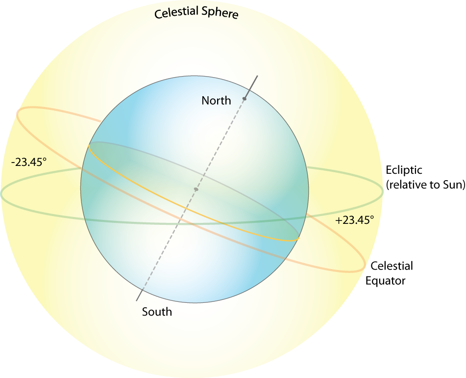
| declination | (delta) | 0o to ± 23.45o; Northern Hemisphere is +ive |
| hour angle | (omega) | 0o to ± 180o; solar noon is zero, afternoon is +ive, morning is -ive |
Sun-Observer Angles
| Angular Measure | Symbol | Range and Sign Convention |
|---|---|---|
| solar altitude angle (complement) | (alphas is the complement of thetaz) |
0o to + 90o |
| solar azimuth angle | (gammas) |
0o to + 360o; clockwise from North origin |
| zenith angle | (thetaz) |
0o to + 90o; vertical is zero |
Collector-Sun Angles
| Angular Measure | Symbol | Range and Sign Convention |
|---|---|---|
| surface altitude angle | (alpha) | 0o to + 90o |
| slope or tilt (of collector surface) | (beta) | 0o to ±90o; facing equator is +ive |
| surface azimuth angle | (gamma) | 0o to + 360o; clockwise from North origin |
| angle of incidence | (theta) | 0o to + 90o |
| glancing angle (complement) | (alpha) |
0o to + 90o |
2.4 Earth's Tilted Axis and the Seasons
Reading Assignment
- SECS, Chapter 6: Sun Earth Geometry (scan through the entire chapter first.)
Please scan all of Chapter 6 right away, to get an initial overview of the role of angles and time together with the relative positions of the Sun, Earth, and the SECS that your client would like to install. We use several angles throughout this chapter (check back to the Table of Angular Symbols [43] anytime, also found in the textbook Ch. 1). We also use a whole lot of dense equations. Don't be intimidated by the equations; they are all based on the trigonometry for a spherical surface, and we will break them down in chunks in this lesson. Just take note of them and keep reading. Take a few notes in the margins as you go!
In this first assignment, we are going to get familiar with the angular relations between the Earth and the Sun, and the relation of those angles to things like Seasons! You are all familiar with the concept that winters are cold, and summers are hot, but why??
Keep an eye out for the cosine projection effect. This is something that we often wish to minimize by tilting our solar energy conversion systems up toward the predominant diurnal (daily) arc of the Sun averaged over the year.
Earth's Rotation
As we have seen in our reading, the Earth rotates with a roughly constant speed, so that every hour the direct beam (a ray pointing from the surface of the Sun to a spot on Earth) will traverse across a single standard meridian (standard meridians are spaced 15° apart). The implications are that the unit of one hour is equivalent to the rotation of Earth 15 degrees. When Earth rotates such that the beam of the sun shifts +1° of longitude from East to West: it takes 4 minutes of time.
- 1 h = +15° Earth rotation
- 4 min = +1° Earth rotation
Wild fact: a time zone change of one hour is really just 15 degrees of separation between standard meridians.
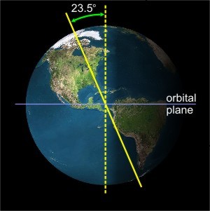
The axis of rotation of the Earth is tilted at an angle of 23.5 degrees away from vertical, perpendicular to the plane of our planet's orbit around the sun.
The tilt of the earth's axis is important, in that it governs the warming strength of the Sun's energy. The tilt of the surface of the Earth causes light to be spread across a greater area of land, called the cosine projection effect.
Cosine Projection Effect
When you tilt a surface away from a beam of light, you spread the same density of light across a larger area. Recall that irradiance is in units of W/m2, so a larger denominator means a smaller value of irradiance, right?
Explore the concept of the cosine projection effect in the following experiment.
Self-Check
This links directly with Chapter 6: Experiment with a Laser of SECS.
Watch the video of the virtual flashlight below and then answer the questions.
Video: Light intensity experiment using a flashlight (0:17)
In this video, changes made to the angle of the flashlight affect light intensity. The shallower the angle, the more the light spreads out, resulting in a lower intensity.
Seasons and the Cosine Projection Effect
The sun is about 93 million miles away from the Earth (equivalent to ~150 million km). That is so far away that the photons from solar irradiation effectively travels in parallel rays. So, unlike the flashlight experiment, the tilt of the sun has no bearing on the intensity of the radiation reaching the Earth's surface. Instead, we find that the Earth's tilt controls the intensity of irradiation and the seasons.
Keep in mind that the Earth's axis points to the same position in space (toward the North Star, Polaris). As the Earth travels in a near spherical (a very small eccentricity into an ellipse) orbit around the sun, the Northern Hemisphere can be tilted toward or away from the sun, depending on its orbital position.
SPRING: (Image of the tilt of the earth in the spring) In this configuration, the earth is not tilted with respect to the sun’s rays (The earth in this picture is actually tilted towards you as indicated by the fact that you can see the North Pole – green dot). Therefore, radiation strikes similar latitudes at the same angle in both hemispheres. The result is that the radiation per unity area is the same in both hemispheres. Since this situation occurs after winter in N. Hemisphere we call it spring, while in the S. Hemisphere it is autumn. This occurs on March 21.
SUMMER: (Image of the tilt of the earth in the summer) When the N. Hemisphere is tilted towards the sun, the sun’s rays strike the earth at a steeper angle compared to a similar latitude in the S. Hemisphere. As a result, the radiation is distributed over an area which is less in the N. Hemisphere than in the S. Hemisphere (as indicated by the red line). This means that there is more radiation per unity area to be absorbed. Thus, there is summer in the N. Hemisphere and winter in the S. Hemisphere. This situation reaches a maximum on June 21.
AUTUMN: (Image of the tilt of the earth in the autumn) In this configuration the earth is not tilted with respect to the sun’s rays (The earth in this picture is actually tilted towards you as indicated by the fact that you can see the North Pole – green dot). Therefore, radiation strikes similar latitudes at the same angle in both hemispheres. The result is that the radiation per unit area is the same in both hemispheres. Since this situation occurs after summer in the N. Hemisphere we call it autumn, while in the S. Hemisphere it is spring. This occurs on September 21.
WINTER: (Image of the tilt of the earth in the winter) When the N. Hemisphere is tilted away from the sun, the sun’s rays strike the earth at a shallower angle compared to a similar latitude in the S. Hemisphere. As a result, the radiation is distributed over an area which is greater in the N. Hemisphere than in the S. Hemisphere (as indicated by the red line). This means that there is less radiation per unit area to be absorbed. Thus, there is winter in the N. Hemisphere and summer in the S. Hemisphere. This situation reaches a maximum on December 21.
Self-Check
Click on "Summer" in the above animation. When the Northern Hemisphere tilts toward the sun, the irradiation has a lower angle of incidence, meaning more photons strike a smaller area during the daytime. Answer the following questions for yourself. If you have any questions, please post to the Lesson 2 Discussion Forum.
- What happens to the Southern Hemisphere?
- What is the correlation with concentrated sunlight and the seasons?
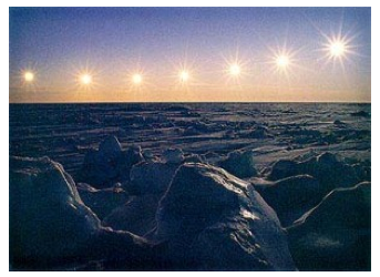
- What happens beyond the Arctic Circle, which spans from about 66.5 degrees latitude to the North Pole?
Now, answer the same questions for autumn, spring, and winter.
Forecasters and meteorologists use different criteria to determine the "meteorological seasons." For example, meteorological winter in PA runs from December 1 to Feb 28/29, a period that statistically includes the three coldest months of the year. This is also centered on a time about 25 days after the Winter Solstice.
Meteorological summer runs from June 1 to August 31, a period that includes the warmest three months of the year. Again, this is a period centered about 25 days from the Summer Solstice.
As one more example, review Pittsburgh's plot of annual average high temperatures. The maximum daily temperature occurs in late July, long after the summer solstice.
Self-Check
2.5 Solar Time and Watch Time
Reading Assignment
- SECS, Chapter 6: Sections titled "Time Conversions"
In this continued reading of Chapter 6, you will be focusing on the way that we account for time in solar energy and the relation of time to more spherical angles. We will use those angles to later calculate the estimated irradiance and irradiation conditions just outside of the Earth's atmosphere (called Air Mass Zero: AM0).
Pay attention to the use of solar time vs. watch time (which will be expressed as standard time vs. daylight savings time). In solar simulation tools like SAM (System Advisor Model), we will only be using solar time, which is the industry norm. Watch time is just a convenient way to get everyone to work at the same time, and to coordinate conference calls. Your job is to get out of watch time and into thinking in terms of solar time, and the angles those times represent.
As we see in the reading, time is a critical parameter in solar energy resource assessment, and we use a "different" time from your mobile phone (or if you have one, a watch). The time that we use in solar energy is the apparent time and path of the sun relative to the aperture or collection device, called Solar Time.
- A solar day is 24 hours long, and Solar noon is always used locally as the center of time.
- Solar noon is defined as the moment when the Sun is at its highest point in the sky.
- The hour angle for solar noon is (given the symbol of lowercase omega).
- Time before solar noon counts backward from , and so the angles are negative.
- Time after solar noon counts forward from , and so the angles are positive.
Correcting Time for Big Longitude Changes: Standard Meridians
The time that you are used to using on your laptops, phones, and (if you still have them) watches is called Standard Time, and is referenced back to the Coordinated Universal Time (UTC), the primary time standard by which the world regulates clocks and time.
Our notion of time is also tightly coupled with our system of longitude (the longitude symbol for us is ). We have used lines of longitude, or meridians, as a reference for time and position E-W. Because time and angles are all linked together, we cannot escape the sexagesimal (base 60 math) system for geographical locations. As we demonstrated earlier in the lesson, each standard meridian (a major line of longitude) is spaced 15° apart, beginning with the Prime Meridian () in Greenwich, England, and continuing for 360 degrees, or 24 hours.
I live someplace other than Greenwich. How do I account for Longitude ()?
Your standard time zone will tell you the standard meridian (). For example, the EST is -5h from UTC, while Central European Time (CET, like Paris) is +1h from UTC.
- For every standard meridian shift to the West, you will need to subtract 15 degrees per hour.
- For every standard meridian shift to the East of the Prime Meridian, you will need to add 15 degrees per hour.
Self-Check
Answer the following questions for yourself. If you have any questions, please post them to the lesson 2 discussion forum.
- Find the meaning of UTC and solar time in Wikipedia.
- Find the acronyms for Standard Time and Daylight Savings time, each in your own time zone today. See timeanddate.com [46] for some help.
- Find the number of hours shift from UTC in your own time zone today.
- How many degrees is the Prime Meridian from your Standard Meridian, and is it the same (or less/more) than the number of hours of longitudinal shift you would expect from the reading?
- Are you in Daylight Savings time now? Would that affect the time correction?
Correcting for Little Longitude Changes: Inside Time Zones
Where you live, or where your future solar site assessment will occur, will likely be well within the edge of a time zone (meaning ). We already learned that every 1° of angular rotation on Earth is equal to 4 minutes of time. Standing in one spot on the surface, this means 4 minutes of relative time correction locally per degree of deviation from a Standard Meridian ( ). So, locales will have a local longitudinal refinement to account for, in order to account for not living directly on a 15-degree incremental Standard Meridian on Earth.
Standard Meridians define the beginning of a time zone, and not the end of a time zone. So, you are always going to look to the start of a time zone to find the Standard Meridian.
There are a few other cities that actually are well seated for solar time zone correction (close enough for our calculations):
- Philadelphia is fairly close to the EST standard meridian of -75°.
- Denver is fairly close to the MST standard meridian of -105°.
My client lives someplace other than a Standard Meridian, how do I account for that?
First, go to Google and type "<insert city name> longitude". You should get a quick response of both the Longitude (lambda) and the latitude (our symbol for latitude is lowercase Greek "phi": phi), represented in decimal form (more useful to us for trigonometry and angles).
Have you noticed that real time zones are more often political boundaries that zigzag around, rather than following an actual Standard Meridian? So, actually, there can be locales for clients that are East of their own time zone Standard Meridian, instead of the normal relative locations West of the time zone Standard Meridian. This is why, in the reading, you will see minutes per degree of local longitudinal shift away from the time zone's Standard Meridian.
Correcting with the Equation of Time: Accounting for Wobbles
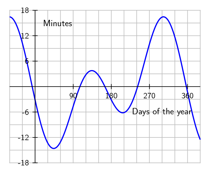
Even in Greenwich, where no longitudinal correction is necessary, "noon" UTC will generally not be the time when the sun is directly overhead. We can see in the plot below that watch time and solar time are the same in Greenwich for only 4 days in the year.
- There are deviations of up to minutes (regardless of your location on the planet).
As you will have read, our interpretation of watch time assumes an even progression for Earth's planetary rotation, with no weebles or wobbles or precession of the polar axis. However, you will now know that wobbling occurs, and there is great variability in the rotation of the earth throughout the months of the year. This is why we add leap years and leap seconds to our calendars. So, we create a "mean time" based on the length of an average day to keep things simple. Solar time has to correct for this mean time approximation. Equation of time correction versus day of the year is shown in Figure 2.7. As an exercise, you can try to calculate these curves based on the empirical equations (6.10) and (6.11) in Brownson textbook.
The following picture was a composite of images, taken at the same watch time every few days for an entire year, to record the position of the sun. We call the shape an analemma. Notice how there is a big loop and a little loop, and compare the same big waves and little waves in the first image of the Equation of Time correction above. If you were to draw a line down the center, you would have removed the error from watch time, and you would be one step closer to solar time.
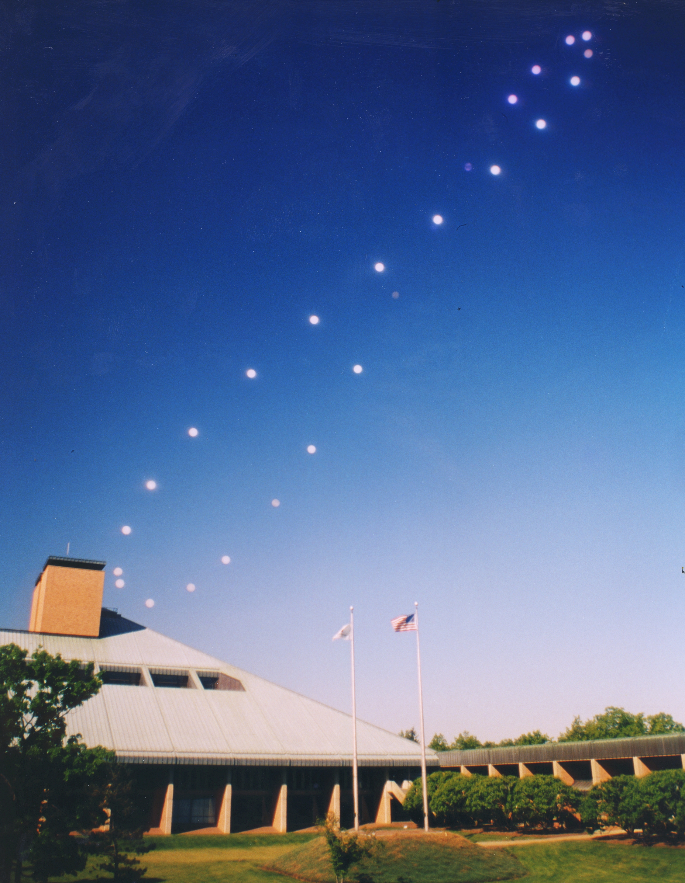
For views of amazing solar analemma photography by Anthony Ayiomamitis, also, please visit the Stanford SOLAR Center [49].
These images were taken at the same time and location every day for one year. You will see the curve described by the Sun over that year. An analemma is a beautiful way to capture both the range of declination $\delta$ (along the length of the analemma) and the Equation of Time Et (the expansion or width of the analemma) in a graphical format.
Putting Time Correction Together:
As we have seen in the reading, we have a method to correct local watch time to solar time, to correct for the true time of day according to the sun relative to the meantime.
The time correction factor is a function of the equation of time, the meridian of the local standard time zone (Lst), and the longitude of the collector/observer (Lloc), and the Equation of Time (Et). The equation of time correction accounts for the wobble and is the first step. Then we need to correct for the change in longitude leading to time zones (standard meridians occur every 15 degrees) and the change of time for locales that are not located along standard meridians.
In these conversions, each year is assumed to begin just after midnight, Dec. 31, and time counts up from there. The time corrections here are in terms of minutes, not hours. The Equation of Time corrects the time to mean solar time (by adding or subtracting up to 16 minutes of correction). The Time Correction Factor corrects time for your shift in Latitude from each Standard Meridian (which occurs every 15 degrees away from the Prime Meridian). Daylight Savings Time is an optional correction, as there is a +60 minute difference from Standard Time between March and November in the USA (and some other regions of the world).
2.6 Let's Convert Solar Time to an Angle
Reading Assignment
- SECS, Chapter 6: Review both sections of "Moments, Hours, and Days" as well as Sun-Observer Angles."
In reviewing these sections, you should notice that three common angular symbols keep popping up: the declination (), the local latitude (), and the hour angle (). As we shall again see in the next section, these are three of our key Earth-Sun angles.
We additionally include the use of longitude () in our calculation of time, and in particular, converting time to an angle: the hour angle.
Now, let's convert "time" into an angle, for our future trigonometric relations:
When we convert time to an angular value, we can no longer use a 24 hr format. We need to convert hourly time into a useful angle based on the properties of a sphere, again using spherical trigonometry.
Video: Hour Angles (5:03)
So, I'm sure a lot of you are wondering what we do with the hour angle. Because it's not something that we really ever used before in regular everyday language. But because so many of our mathematical calculations are in terms of angles, remember, angles are coordinates in the solar reference in the solar frame of reference.
So, when we normally have 24-hour time, we need to convert that time into something on the order of 360 degrees or, in our case, minus 180 degrees to plus 180 degrees. And so, we're going to figure out a way to convert 24 hours of time to degrees. And those degrees are going to be found as the hour angle.
So, time is going to be in terms of decimal hours. So time in decimal hours. And we're going to make sure that we do that in a 24-hour time frame, so that if I were talking about 1:30 in the morning, I would represent this as 1.5. If I wanted 1:30 in the afternoon, based on the 24-hour system, that would be 13.5. So we have that understood.
So, in order to get the hour angle of time, we're going to start with time is going to be the hour angle times the conversion of one hour per 15 degrees of rotation of the earth. So that's going to give me my decimal hours-- multiplying right there-- such that if I wanted to have the hour angle, I would have time times 15 degrees per one hour. In which case, my time is in hours. The units of hours would cancel out. And I'd be left with units of degrees.
Now, one of the things that you're going to find in your problems is the calculation of day length. And if the day length in the textbook is shown by calculating the hour angle of the sunset-- and we do sunset because it's a positive angular value. Basically, if I were to-- here, let me do a quick diagram.
If I were to put noon, 12:00 noon here, any time before noon would be negative. Any time after noon would be positive. So, this is where I have my negative 180 degrees going into the morning. You're looking back before noon, so you have negative degrees. Going into the afternoon, you're going after 12. So, you're adding degrees. So it's positive.
So, I have a positive value for the sunset. So, if I wanted to calculate the sunset, we find that I need to calculate the arc cosine or the inverse cosine of the negative tangent of the declination times the tangent of the latitude, phi. And I might have switched these two guys around in the textbook. But you're going to get the same answer.
So, that will give me the time of sunset or the hour angle of sunset. And the hour angle of sunrise is going to be the negative of the sunset. And then the last part that you're looking for, hours in a day, is going to be 2 times the sunset hour angle times the conversion of one hour for 15 degrees. That's going to give you the number of hours in the day. And you're going to want that for one of your answers as well.
Finishing Step for Time Conversions! The Hour Angle () in decimal degrees.
We represent the apparent displacement of the sun away from solar noon, either as a negative or positive angle. An of zero indicates that the sun is at its highest point for that given day.
- The sign of the hour angle before noon is negative, because we have to count backward from the "zero hour" of solar noon.
- The sign of the hour angle after noon is positive, because we are counting forward from the "zero hour" of solar noon.
Another way of looking at it is the angular difference between the local meridian of the observer/collector and the meridian that the beam of the sun is intersecting at a given moment.
Now, the day won't really begin at -180 degrees, anywhere between the arctic circles. However, I wanted to emphasize that the day only begins at -90° on two days a year. Those days occur during the Equinox moments in the orbit of the Earth about the Sun, and the length of those days is actually 12 hours long. All other days are either shorter than 12 hours, or longer than 12 hours. As such, they end either less than 90° or greater than 90°.
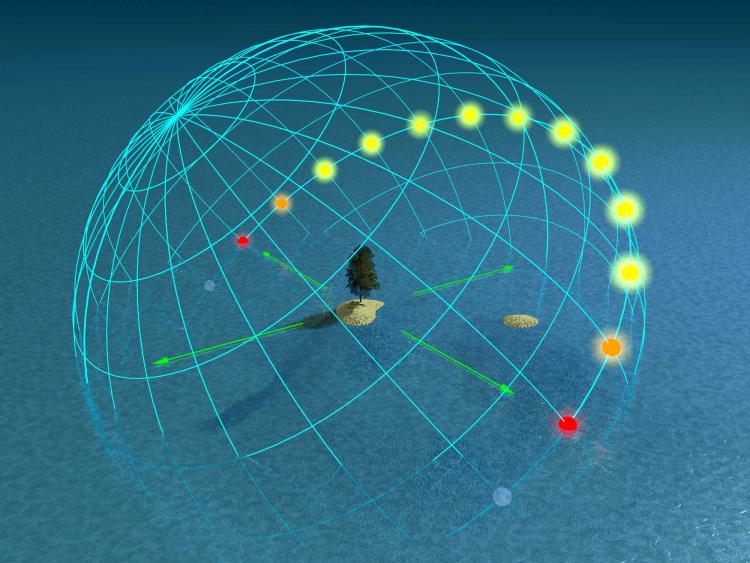
The images below demonstrate singular arcs of the Sun for each hour in solar time, at five different latitudes on Earth (no analemma correction necessary). The peak hour (or the hour with the highest solar altitude angle) is defined as solar noon. You will notice that the solar equinox has twelve sun spots for latitudes below the arctic circle, and that the sun rises due East, while setting due West. During the solar solstices, you see multiple arcs: one for winter and one for summer. Notice that there are more hours of the day in the summer, and the sun rises farther from the equator in the Summer (sun rise in the northeast for the Northern Hemisphere).
What else do you notice in comparing the four critical times of year at different latitudes?
Solar Equinox
 [52]
[52]  [53]
[53]  [54]
[54]  [55]
[55]  [56]
[56]
Solar Solstice
 [57]
[57]  [58]
[58]  [59]
[59]  [60]
[60]  [61]
[61]
Now, we are ready to use hour angle to find out positions in our solar design projects!
Self-Check
2.7 Let's Convert Time from Watch to Solar
Remember that the Earth rotates at 15 degrees per hour, and 0.25 degrees per minute. It can get confusing when you're comparing spatial seconds with temporal seconds, right? That's why we will stick with decimal notation in all of our references to latitude ($\phi$), longitude ( ), and angles (degrees).
Self-Check
Step 1: Correcting for Standard Time (Standard Meridian) in Hours: Find the time zone of your client. The hourly longitude correction is plus or minus X hours from the Prime Meridian, where UTC = 0h. Multiply the positive or negative hour value by 15°, and you will know your standard meridian for the Time Zone.
Key: Your standard meridian for your time zone begins on the East side of the time zone. (Sun rises in the East, right?)
Step 2: Correcting for Time from the Local Longitude Relative to Standard Meridian in Minutes:
You need to know the longitude for the standard meridian of the client ( ) from their local time zone, and the local longitude of the client's location in question (). We calculate the longitudinal correction, from these two.
Keep in mind: Time zone borders are political boundaries, and can be constructed on both sides of a Standard Meridian. A locale to the east of the Standard Meridian would still be input as a positive value (the resulting minutes would be positive).
Note: we use the sign convention that longitudes are positive valued for to the East of the Prime Meridian, and negative valued to the West of the Prime Meridian. This equation is valid for both sides of the Prime Meridian. The exterior negative sign is there to make the time correction algorithm work correctly.
Step 3: Calculating Equation of Time (Analemma) Correction in Minutes (Et): We begin with the two simple coefficients of n (the day of the year, from 1-365), and B (see the first equation). Our assumption is that the year begins at midnight of the new year, and the trigonometric portions of the equation of time will take an argument of "B" in degrees.
You have seen that the Equation of Time has a graphical representation, the analemma. Once we determine a correction in the scale of minutes, we can use it in the Time Correction Factor, TC.
Step 4: Completing the Time Correction Factor ($TC$): The time correction factor is a time shift in minutes.
Recall that 0.25° of longitudinal rotation (of the planet) will consume 1 minute of time. That would make each degree of change equivalent to four minutes. Hence, we need to multiply our longitudinal correction by a factor of four to yield a consistent unit of minutes in time. This is shown as the value of the longitudinal correction (Lc) in units of minutes (temporal, not geospatial).
Step 5: Accounting for Daylight Savings Time (DST) in 60 minutes.
The equations do not tell you when DST occurs from country to country. There is a +60 minute difference between March and November in the USA. So, if we had to correct for DST, then we would need to subtract that 60 minute addition back out.
Again, make sure that the data is presented in minutes, rather than hours.
Self-Check
2.8 Discussion Activity
Continuing Conversations in Yellowdig!
I hope you are getting the hang of Yellowdig conversation platform and are ready to pick up the pace! You can access the discussion platform through the Canvas menu.
Lesson 2 Discussion: Reflection on Time Conversions
For this week, I would like you to question why we do all of these time conversions for solar energy. Why do we need to know these time and angle relations as solar energy specialists? There are many terms and concepts to reflect on – some are well-known, and some may be new to you. In this discussion you will have a chance to reflect on the meaning and your understanding of those and perhaps some of your peers’ interpretations of those concepts will be helpful to your comprehension of this lesson. Here are some guiding questions you may use as starting points for your posts:
- What is the difference between Solar time vs. Clock time? Is that important, significant, and should we bother?
- Analemma, what is it representing, and how it affects the solar time?
- What is longitudinal time correction?
- Daylight savings - what insight have you gained about the use of daylight savings in society? Is it useful, not so much, meh?
- What are equinox and solstice's role in solar resource forecasting? These are key, critical points in time. What makes them special?
This is an open-ended discussion, and you may ask questions or raise your concerns with things that might still remain confusing. Feel free to post and comment on any of the above-listed topics and whatever you want to share after working through the lesson material.
Tagging
Yellowdig Tip: When you create a post in the Yellowdig discussion space, you are required to choose a topic tag. For Lesson 2 discussions, use any of the following:
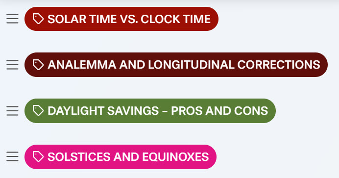
Know that you can tag your post with one or several of these topics depending on its content. It gives you flexibility to discuss these things cumulatively or, if you prefer, to break your writing into several smaller posts.
Importance of interaction
Once again: the more you participate, the more opportunities for your discussion score to grow through the week. Comment, ask questions, react, throw in additional thoughts – it all is in your benefit!
Grading
Yellowdig points you earn over the weekly point earning period (from Saturday to next Friday) will count towards 1000 pts. weekly target. But you can go above it (to 1350 pts. max) if you are feeling active. That may help you to make up for some low-activity weeks. Yellowdig discussions will account for 15% of the total grade in the course. Check back the Orientation Yellowdig page in Canvas for more details on the points earning rules.
Deadline
There is no hard deadline for participating in these discussions, but I encourage you to create your posts in the middle of the study week (Sunday) to allow others to engage and respond while we are learning specific topics in the lesson.
2.9 Sun-Earth Relations
Reading Assignment
- SECS, Chapter 6: Earth-Sun Angles section
The following sections are closely coupled to the reading assignment, but I have enlarged the images for you. Our Solar Energy Conversion Systems are going to be fixed at some location on the surface of Earth, right? So, we will place an "Observer" at the future location and describe the relative position of the Sun and Earth and SECS. However, there are a few underlying spherical relations that do not depend on the location of the SECS or the observer.
This section discusses those geometric relations that are effectively "Independent of the Observer." Keep an eye out for the declination (delta, ), the latitude and longitude ( and ), and , the hour angle.
The Greek notation used below is now fairly standard for the field, but you may see different approaches in informal settings or unusual textbooks. I follow the established nomenclature defined by Beckman, et al., in the research journal Solar Energy in 1978, reprinted in Solar Energy in 1997. As noted earlier, the document is available to you from the Library E-Reserves.
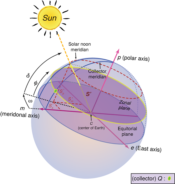
Hour Angle ():
Again, this is the way we represent the apparent displacement of the sun away from solar noon. An hour angle of zero degrees indicates that the sun is directly above, and the sign of the hour angle is determined by occurring either before noon (negative) or after noon (positive). Another way of looking at it is the difference in angle between the local meridian of the observer/collector and the meridian that the beam of the sun is intersecting at a given moment.
Angle of Declination ()
This is not an observed angle relative to the surface of the Earth and the Collector. Declination is the observed angle (due to the polar tilt) between the plane of the Earth’s equator and the plane of the ecliptic (the plane in which the Earth's orbit about the Sun lies). Declination has a maximum angle of 23.45° at either solstice. In this case of coordinates, the sun observed in the North is positive, and in the South is negative. One can imagine this as a series of sun paths over the course of a year. In contrast, the declination reaches a midpoint at either of the equinoxes. The range of declination is limited to Earth’s tilt: −23.45° (winter solstice) (summer solstice).
Declination is independent of location on the planet!
The declination can be calculated by a simple approximation (first equation) or a Fourier series (second equation).
where:
Angle of Latitude () and Longitude ()
The complement of longitude () in geospatial coordinates is the latitude. When combined together, we have identified a singular point on the surface of Earth. However, separately, they refer to arcs or circles spanning huge distances. We can look up the latitude and longitude of a site on a search engine like Google.
Key latitude angles of interest are:
- Arctic Circle = +66.56° North of this, the sun is above/below the horizon for 24 continuous hours at least once per year (during the solstices).
- Tropic of Cancer = +23.45° The maximum tilt of the North Pole to the Sun.
- Equator = 0°
- Tropic of Capricorn = −23.45° The maximum tilt of the South Pole to the Sun.
- Antarctic Circle = −66.56° South of this, the sun is above/below the horizon for 24 continuous hours at least once per year (during the solstices).
2.10 Sun-Observer Relations
Reading Assignment
- SECS, Chapter 6, Sun-Observer Angles section
Once we have identified our specific location on the surface of Earth, we use the spherical relations between the Sun and the fixed observer at the locale to describe the relative motion of the Sun during the day and over the year. Once again, this text is closely complementing the text in the book.
Pay attention to the fact that this particular set of relations is only for the special case of a horizontal surface. We are only describing angles for an imaginary flat surface on Earth, like a table top. In real SECSs, we will often tilt the receiving surface up (tilt has a symbol of ), specifically to minimize the cosine projection effect that occurs at a given latitude. Bear in mind that the angles for a non-horizontal surface (tilted, with some accompanying azimuth orientation ), or for a tracking system, are an entirely different set of general equations.
Also, as these relations refer to the apparent motion of the Sun, they have the subscript of "s" for the two coordinate angles of solar altitude angle and solar azimuth. The complement of the solar altitude is the zenith angle, which has a special subscript of "z".
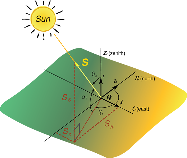
The Solar Altitude () measures the angle between the central ray from the Sun (beam radiation), and a horizontal plane containing the observer. Note that the subscript "$_s$'' is there to indicate that the altitude relative to the observer of the Sun. This will become important in evaluating the altitude angles of other objects projected onto the sky dome, like buildings, overhangs, wing walls, and arrays of solar receivers.
The Zenith Angle () is the geometric complement of the solar altitude angle. We direct your attention to the use of here, as the general concept of the angular deviation of the Sun's ray from the normal projection of a surface is called the angle of incidence, . In effect, the zenith angle represents the angle of incidence for a horizontal surface.
Recall: "normal" means perpendicular to a surface.
The Solar Azimuth () measures the angle on the horizontal plane between the meridian of the 0 degrees axis (South, for the Northern Hemisphere, opposite Down Under) and the meridional projection of the Sun's central beam (the Sun's meridian). The convention we will use is also used in the advanced design tools for solar energy, TRNSYS (UW-Madison: Transient eNergy Simulation Software), PVSyst, and SAM (NREL: System Advisor Model). The angle varies from 0 degrees at the South-pointing coordinate axis to degrees. East (earlier than noon) is negative and west (later than noon) is positive in this basis. This is a well-used standard taken from the original text of M. Iqbal.\cite{iqbal83}
Note: the function "sign()" is specifically defined as a cases form of positive and negative notation (meaning there are two alternate cases to choose from).
There are several texts and software available that use a solar azimuth, measuring clockwise on the horizontal plane from a North-pointing (0 degrees) coordinate axis. This is also the convention for the field of meteorology and for the wind industry. This azimuth convention uses 360 degrees for the meridional projection of the Sun's central beam.
However, the majority of professional software does not use this convention yet, so you must be aware of the difference, as the math changes with the two methods. It is relevant to be aware of the difference, in that the North basis is used in the basic educations tools for simulation called PVWATTs, for the sun path tool at the University of Oregon, and in the interactive software PVEducation.org [21].
2.11 Collector Orientation
Reading Assignment
- SECS, Chapter 6: paying attention to sections of "Collector-Sun Angles" and "A Comment on Optimal Tilt"
Once we have identified our specific location on the surface of Earth, and used those coordinates to identify the location of the Sun in the skydome relative to a fixed observer in a given locale, we can enter the angles for the orientation of our SECS. Again, this text closely complements the text in the book.
What is different here?
This new set of relations is for the general cases of any surface (horizontal or tilted, fixed or tracking). We are now describing angles for real oriented surfaces on Earth, like tilted PV panels and walls of a building. As we noted in the last section, for real SECSs, the receiving surface is tilted (beta, , with an azimuth orientation γ) to minimize the cosine projection effect that occurs at a given latitude.
Also, pay particular attention to the angle of incidence (theta with no subscript, ). As part of a solar energy design team, one of our primary mechanisms to increase the solar utility for the client in a given locale is to minimize the angle of incidence at a given time during the year or day. This is an extension or refinement of reducing the cosine projection effect.
Finally, I will give you a heads-up for the next page: after reviewing these sections and completing this page, you will need to take the Lesson 2 Quiz. Note that this is a quiz with calculations, and you will likely want to have a numerical software open to work through the numerical problems.
The following angles describe the orientation of the collector surface and the relation of the collector surface to the Sun. As these three angles describe our primary surface of interest, the SECS, they do not have a subscript for the two coordinate angles of collector tilt and collector azimuth.
- Tilt: the angle between the plane of the collector (or aperture) and the horizontal. Denoted by the symbol beta, β.
- Azimuth: the planar rotation East or West that an aperture will have. Denoted by the symbol gamma with no subscript, .
- Angle of Incidence: the angle between the vector perpendicular to the collector plane, called the normal of the plane, and the projection of the Sun’s central beam to the collector surface. Denoted as theta with no subscript ().
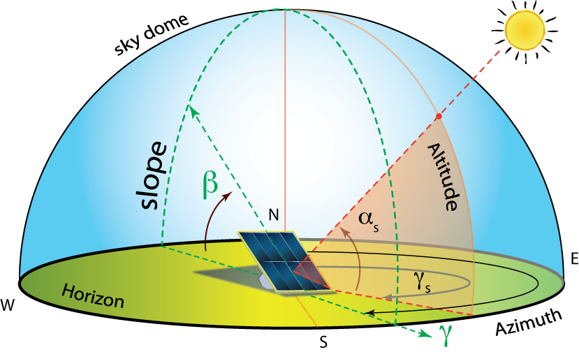
For general cases, where the collector has a non-horizontal orientation (), the angle of incidence is not the same as the zenith angle (θz). In fact, the zenith angle is a special case of an angle of incidence for horizontal surfaces, where the zenith is referenced to the aperture as a normal projection.
The first and second angles of tilt and surface azimuth (and γ) are typically known for fixed surfaces. The third key angle is the angle of incidence (θ), which uses the following rather lengthy equation:
In order to generate an actual value for theta, we will need to also take the arccosine of the long equation. For your calculators and math programs, all of the arguments are in terms of degrees, not radians. You will need to convert degrees to radians in most programs.
However, this is a really long equation that can actually be broken down into parts. We will break up the equation for the angle of incidence (theta, ) into three lines. Take a look at them, and look for common arguments to the sine and cosine functions.
- ( , , : latitude, declination, and tilt)
- ( , , , : latitude, declination, tilt, and then collector azimuth)
- ( , , , , : latitude, declination, tilt, collector azimuth, and then the hour angle)
Mechanisms to Maximize Solar Utility:
In the introduction of the textbook, there is a reference to the goal of solar energy design: to maximize the solar utility for a client in a given locale.
There are three main design mechanisms that will increase the solar utility of a SECS for a client or group of stakeholders.
- Decrease the cosine projection effect: This is done by tilting the collector toward the Sun's average annual noontime position. The higher the latitude of the locale, the more tilt a collector will need. Seasonal tilt changes can also slightly improve the solar gains. We also direct the collector toward the equator, although there is significant flexibility in both tilt and azimuth.
- Minimize the angle of incidence: This is a refinement of the first mechanism over the course of a given day, particularly relevant to solar tracking systems. By "pointing" the collector normal at the Sun during the day, the angle of incidence is minimized, and more light can be collected.
- Minimize or remove shading effects from the collector: We will cover this in the next few pages. It should make sense that when shadows cover a collector, then the majority of the Sun's light for that unexposed area is no longer providing power. Photovoltaics will be much more susceptible to shading issues than solar thermal systems, due to the near instantaneous generation of charge carriers in PV vs. the slower reaction from a thermal response of fluids.
2.12 Siting using Sun Paths and Spherical Coordinates
Reading Assignment
- SECS, Chapter 7: Applying the Angles to Shadows and Tracking
This is a brief recap to set the stage for orthographic projections and polar projections used in the shading analysis project to come.
In a spherical coordinate system, the angles are the coordinates. So, if I were standing in a field in North Dakota, looking at something tall like an enormous wind turbine, I could define the position of the top of the nacelle relative to me by stating the general azimuth angle (, the rotation across the horizon from due South) and the general altitude angle (, the rotation up from the horizon). Effectively, this is my x () and y () coordinates on an orthographic projection of the sky dome on a flat surface.
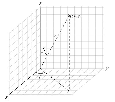
Many of you will be familiar with Cartesian coordinates in space (x, y, z). However, when dealing with spatial relations of spherical objects like the Earth and the Celestial Sphere, we find that working with basic spherical coordinate systems makes trigonometry available to us to solve for space and time equations. For spherical coordinates, we need information of radial distance, zenith angle, and azimuth. However, in solar positioning studies, a radius of one (unit radius) is all we need to establish a unit vector, and we are left with equations for only the zenith angle and azimuth (and the complement of the zenith angle, the altitude angle). Note how the zenith angle in Figure 2.15, above (the generic angle), is congruent with the solar zenith () of the Sun, and the generic azimuth angle () is congruent with the solar azimuth ().
The following equations describe the Cartesian coordinates (x, y, z) for unit vectors, followed by the equivalent functionals using the complementary altitude angle.
As seen in Figure 2.16, we need to pull back to our old trigonometry mnemonics! Recall "Soh Cah Toa" when looking at the figure:

- Sine(A): Opposite over Hypotenuse (a/h)
- Cosine(A): Adjacent over Hypotenuse (b/h)
- Tangent(A): Opposite over Adjacent (a/b)
2.13 Sky Dome and Projections
Sun Charts: Projections of Solar Events and Shadowing from the Sky Dome
The emphasis of this lesson is the Sun Chart tool (or Sun Path). These flat diagrams are found in many solar design tools, but may look completely foreign to the new student in solar energy. How do we interpret the arcs and points plotted on a sun chart? Why do we have two different types of plots (one looks like a rectangle, and one looks like a circle)? Why do some plots go from 0-360°, while others go from -180° to +180°?
Video: Angles Sunchart 1 (4:45)
OK, we're going to do a little preliminary review of where we've been and why these angles are important to the measurement or the plotting of sun charts. So, we know that we have a set of several earth, sun angles. So, earth, sun angles. Excuse my wonderful writing. And we're going to break those down into the latitude phi, the longitude.
So, we've got latitude and longitude. And we're also going to need the declination, the declination which is going to be a function of the day number n, and the hour angle. And the hour angle, again, is omega. And that's going to be just converting time into an angular value, which we do for the location at hand.
So, along with those earth, sun angles, we have our sun observer angles. And the sun observer angles is going to be broken down into just three simple angles which is going to be the solar altitude, altitude angle alpha with the subscript s relating it to the behavior of the sun. Gamma s is going to be the azimuth angle of the sun. And the third angle is going to be theta z which is the zenith angle for the sun.
Now, I'm going to use the information from latitude, longitude, declination, and hour angle to ultimately calculate the sun observer angles over here. The important angles for our future shading plots and for our sun path diagrams are going to boil down to plotting altitude and azimuth.
So, we're going to use these earth, sun angles to calculate sun observer angles right here. And if we plot those angles over the course of the day, over the number of hours in a day, we're going to ultimately plot the altitude and azimuth angles according to their hour angle. And the complement, of course, of the altitude angle is the zenith angle. I forgot to mention that.
But we're going to be able to make these plots that are going to look like this. They're going to be a square plot where on the x-axis, we're going to have a plot of azimuths. And on the y-axis, we're going to have a plot of altitude angles. So, the altitude angle will go from zero to 90 degrees.
And depending on the system that we're using, negative values might be to the west and positive values-- or negative to the east and positive to the west. We could also plot here the complement. From zero down to 90 would be theta z, just so we know.
And again, if I plotted the solar altitude and solar azimuth angles, what I'm going to get is a plot of the arc over the hour angles. And this lower plot will be for winter, when the sun is low in the sky. Low in the sky means a low altitude angle. When the summer comes, the sun is high in the sky. And so, we have a higher angle in the summer.
And basically, this boundary from here to here is going to be the winter solstice and the summer solstice. These plots are basically plotting a series of altitude and azimuth angles for our sun charts. We will next be plotting a series of angles for shading that we will use.
So, that's our basic overview. Let's go on to the next stage.
What are Sun Charts?
If we want to visually convert our observations of the sky-dome onto a two-dimensional medium, we can either use an orthographic projection or a spherical projection on a polar chart. These projections are useful for calculating established times of solar availability or shadowing for a given point of solar collection.
The Sun Path describes the arc of the sun across the sky in relation to an earth-bound observer at a given latitude and time.
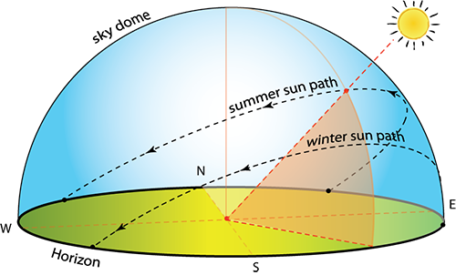
All light incident upon Earth's surface must pass through the atmosphere and be attenuated (lost from absorption or back scattering). In order to simplify the many points of origin of light, we divide the sky and the Earth's surface into components, or spatial blocks of an imaginary hemispherical projection on the sky. The Sky Dome refers to the sum of the components for the entire sky from horizon to zenith, and in all azimuthal directions. In our following sections, a collecting surface is assumed to be horizontal first, as a pyranometer measuring device is mounted horizontally and facing the sky to measure the Global Irradiance/Irradiation in the shortwave band for the sky dome. Most of our solar collectors will be tilted up from horizontal in some way (PV, solar hot water, windows, walls, even your eyes). Those surfaces oriented otherwise are termed a Plane of Array measurement (POA), requiring specific tilt and azimuth information in the description. For those solar collecting surfaces that are not horizontal, the reflectance of the ground is an additional source of light, through the albedo effect. The beam, sky diffuse, and ground diffuse light sources incident upon the tilted collector are estimated using models of light source components.
Projections
The sky dome can be projected onto flat surfaces for analysis of shading and sky component behavior.
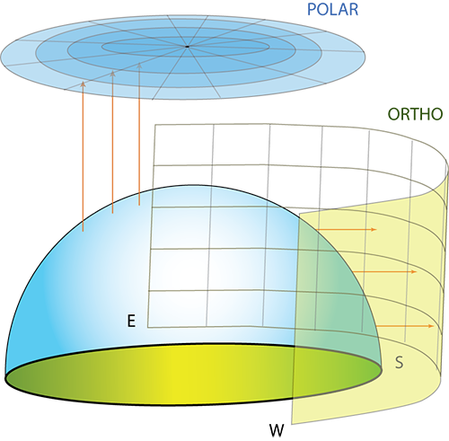
Video: Angles Sunchart 2 (6:01)
So, if we go back and we think about the Sky Dome-- and I'm going to do this little diagram of-- this is the Sky Dome that we've talked about in the textbook and in the class. And this is going to be the ground. And so we have this Sky Dome.
And you can kind of see that this dome that we have could be-- is a hemisphere, first of all. And we could project that dome onto multiple different surfaces.
So, the first projection that we will do is going to be orthographic. And essentially, an orthographic projection is going to be what happens if I were to try to take a flat piece of paper. maybe like a cylinder of paper, and I were to try to wrap that cylinder right around this Sky Dome.
So, I'm going to have-- everybody see the cylinder that's wrapping around? So, I'm going to want to project points onto that flat surface. And ultimately, that flat surface is going to be printed out.
And we're going to have our basis for our sun charts in terms of the azimuth angle. So, the rotation along here, along the plane or rotation along the horizontal is the azimuth angle. And the angle from the ground up, the vertical rotation, is going to be the altitude angle.
Of course, the complement of that, if we were talking about the sun, would be the zenith angle. Which is why we could represent this is 0 to 90 and 90 down to 0 with the zenith angle.
We have two conventions for plotting the azimuth angle. The one is to make east negative. So, we can go negative 180 degrees. And west positive 180 degrees. Where this 0 is pointed at the equator.
The alternate is to begin in the north with 0 degrees and to work your way clockwise to-- all the way around to 360 degrees, in which case south, not the equator, is going to be positive 180 degrees.
Now, this is the convention that a lot of the solar world has used for some time. However, this is the standard convention that has been established through meteorology. And so, we tend to use both flexibly. But just know that, in general, the 360 degree is an accepted standard.
So, if we then go to the next page and we think about that same Sky Dome. And got our ground. And instead of trying to project it off to the side, we are effectively lying on the ground. And we're going to project upwards.
And this way, the azimuth angles are rotating around in a circle just like the azimuth angles will be doing here on the ground.
The altitude angles, however, are going to be represented as arcs across where the higher in the sky you are, the closer to the center of the circle.
And how do we see that? Well, we look at it like this. And we're going to start to see a center point. And I'm going to put south here. We know that south is in the northern hemisphere where the sun is at its highest point.
So, we're going to see arcs in the sky that look like this going from-- in our case-- east to west. This is going to be summertime. This is going to be wintertime. When the sun is low in the sky versus high in the sky.
Here is going to be an alpha 90 degrees. And the ring around the bottom is going to be an alpha of zero degrees. It's a little different plot. The lines are going to be flipped from what you were used to in an orthographic projection, if you can do both of these at the Oregon site for sun plots.
- Orthographic Projection: takes the sky dome and projects altitude and azimuth values outward onto a surrounding vertical cylinder. The cylinder is then opened flat. Figure 2.19, below, shows the sun rising in the East (to the left) and setting in the West (to the right). Proper observation shows that the largest arc in the chart at the top, June 21, is the Northern Solstice, while the smallest, December 21, is the Southern Solstice.
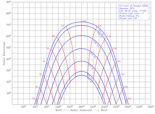 Figure 2.19: Orthographic Projection.
 - Polar Projection: takes the sky dome and projects altitude and azimuth values down onto a circular plane. However, in the polar projection, the arc for December 21 is at the top while the arc for June 21 is at the bottom. This happens because we are effectively lying on the ground with our heads facing south, and holding that large piece of paper straight up to the sky.
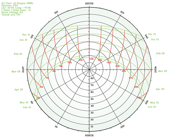 Figure 2.20: Polar Projection
How do We Make and Read Sun Charts?
Go to the University of Oregon Solar Radiation Monitoring Laboratory [64] website. The scientists at the site have provided an excellent tool for plotting sun paths onto orthographic projections or polar/spherical projections. The default page is for creating an orthographic projection of your site of interest. The alternate page for polar projections [65] will use the same data you can input, but will output the alternate form. Note that both use the meteorological standard for azimuth angles, where North is set at 0°, increasing clockwise to 360°.
- Specify the location by and . (Latitude is important for our calculations of sun-observer angles).
- Specify the time zone (software does the correction from UTC to local time zone).
- Choose data to be plotted (Choose to plot hours in local solar time: default). These plots are symmetrical for half of the year when you plot them in arcs of solar time. Hence, when you plot in solar time, "Plot dates 30 or 31 days apart, between solstices, December through June" will look the same as "Plot dates 30 or 31 days apart, between solstices, June through December." Side note: if you do plot in "local standard time," you will observe half of an analemma each hour, where only the Equation of Time ($E_t$) has not been corrected for in the time correction.
- Set chart format parameters: These are your choice to personalize the output file. Be creative, and try to present clear data visualization.
- Choose file format for chart. (I prefer the PDF for working.)
- Enter the code to make sure you are not a web bot roaming about.
- Download the image, print it out, and use it for shading analysis!
What about Shadows?
When designing a solar energy conversion system for any application, we must pay special attention to the occurrence of shadows throughout the year. We discuss a method to assess the shading using 2-D projections.
The next page gives you an opportunity to print and analyze your own sun chart.
2.14 Try This! Print a Sun Chart
Try This! - Print a Sunchart.
Go to the University of Oregon Solar Radiation Monitoring Laboratory [66] [64]web page and generate a PDF SunCharts for two locations: (1) State College, PA, and (2) your own location.
1. Download the PDF chart for the orthographic (Cartesian) projection
2. Download the PDF chart for the polar projection
3. Reflect on the charts:
- Can you find key solar days on the chart (equinoxes, solstices)?
- Can you identify sunrise and sunset solar times for different months?
- How does the position of sunrise and sunset vary throughout the year?
- How are these charts different between your location and State College, PA?
Now, based on your understanding of the SunCharts, work through the self-check questions below. While you work through these steps, try to think about all the calculations that went into each plotted point on the curves. You should reflect on the fact that the SunChart tool is simply plotting points and lines based on solar calculations of time and longitude. The same calculations that you are mastering now in class. Pretty exciting!
Self-Check Questions - based on the SunChart for State College, PA
Answer the same questions for your own locale. Are the answers different or the same compared to State College, PA?
2.15 Applying Shading to a Solar Chart
Reading Assignment
- SECS, Chapter 7: Applying the Angles to Shadows and Tracking
Here, we are going to work through a problem of plotting critical points of shading onto an existing sun path diagram. Keep in mind that we will use the plots that you developed from the University of Oregon Solar Radiation Monitoring Laboratory [66] on the previous page of this lesson.
Here, I am using a program called Skitch [67] to draw over the top of my PDF files. There is a 30-day free trial of the editing software if you would like to use it to digitally mark up your documents. Otherwise, I recommend that you print out your work, draw on the print directly with a pen, and then take a snapshot of the edited image with your phone or scanner to upload.
Quick review of the Charts:
First, we will go over the key features of the orthographic plots with the arcs of six days plotted out for the first half of the year.
Video: Sunchart Ortho Intro (4:42)
All right, so, here we have a sun path diagram of State College, Pennsylvania. We've developed this in the University of Oregon's website for our local latitude and local longitude, time zone UTC minus 5 hours. That's Daylight Standard Time, not Daylight Savings Time. And I've done a little bit of modification to this to give it the green background. So, this is not something that normally you would see inside of your normal program.
But, I want to point out a few things. One is that we see that, as discussed before, the sun rises in the east. And the sun sets in the west, right?
So, we're going to have a progression of the sun across the day from left to right. In this particular case, we start out with east on the left, west on the right. South is denoted by 180 degrees, right?
And so, the thing that I wanted to point out here is that here we have December at the bottom and June 21 at the top. So, this December 21 is the winter solstice. June 21 is the summer solstice. And, in between, we have right about March 21 through the 23 is going to be one of the equinoxes. The other equinox, of course, is going to happen in September.
Only half of the year is shown. The arcs that you're seeing here are all the hours of the day interpreted as solar time. So, this is going to be 10 o'clock solar time. We're using a 24-hour system here. So, this is going to be 2 o'clock solar time, right?
And when I look at this, I see that I have two key points-- 90 degrees and 270 degrees. 90 degrees, of course, is going to be due east. And 270 degrees is due west, in this particular meteorological standard for the azimuth directions.
We see that on the left side, we have the altitude angle. That would be alpha. And we're counting down for the zenith angle, the complement to the altitude angle.
Let's go back to this east and west. So, when does east happen? East happens at due east, is 90 degrees. Due west is 270 degrees.
What's really important here is when does that happen? You see that there's an arc right along here for March 21. And that's really close to the equinox. So, during the equinox, we have the sun-- that's the only time of the year-- so, two times during the year when the sun rises due east and sets due west.
And if we count the hours, we have-- one, two, three, four, five, six-- exactly six hours in the morning-- one, two, three, four, five, six-- exactly six hours in the afternoon, so, a 12-hour day, our only 12-hour day that's going to happen. Otherwise, all of the rest of this time if we're looking at-- let's grab a color here. If we're looking at all of this time of the year from December to February and after March, so, before March is down here. After March is up here. So we're going to have short days, shorter than 12. And we're going to have longer than 12 hours up in the summertime.
Gives you a brief breakdown of what's happening on orthographic projection. This is for State College, of course. As we go further north, we're going to see that our sun charts are going to get lower to the ground.
If we were to choose a latitude location that is closer to the equator, we're going to have plots that start to look like this, actually. They're going to look really kind of funny because they're going to spread out up into the 90 degree space because once you're within the tropics, you're going to find that the sun can be to the north or to the south. It's not always in the south as it is when you're beyond the tropics. Anyway, I hope that's a helpful explanation and--
Second, we can compare the key features of the orthographic plots to the polar plots, again with the arcs of six days plotted out for the first half of the year. You should notice the similarities (East is on the left, solar time is represented, the same location is plotted), as well as the distinct differences (the June and December arcs are "flipped").
Video: SunChart Polar Intro (5:49)
All right, and now we got the same location. Again, the location is going to be State College Pennsylvania. Solar time is going to be minus 5 hours, relative to UTC. And latitude longitude is the same.
Again, this is a polar plot of the same data that you just saw in the previous video. And the north of this plot is right down at the bottom. The south is up at the top. And I do this in this particular case, just to keep the arcs in the same general direction. But you're going to notice some differences here.
One is that the June arc is at the bottom. Whereas the December arc is at the top. So, this polar projection is what you would get if you were effectively lying on the ground and looking at the sky with a fisheye lens. And then trying to project that flat.
So, we see here that we've got the arcs of the day the morning begins over here. The evening ends over here, right in June time. And the progression of the day is going to be across the arc, again, from left to right, the same thing as we had before. Left to right in the winter months as well.
But here, you're really seeing the differences in the length of the day. It's probably a lot more apparent here that the length of the December 21st day is much shorter of an arc then the summer solstice on June 21st. Again, our arrows just pointing out, these green arcs are days. And the red lines are the hours of the day in solar time.
So that this top location here at 90 degrees, is going to be the top of the sky, the zenith. So, the zenith angle is basically any angle down from here to one of these circles. Whereas the altitude angle is going to be the angle up from the ground, which is going to be in our case the edge of the ring up.
So, we're going to see in a zenith angle going down or going outward, two rings. An altitude angle coming up or inward, basically coming along the edge of that skydome. And any one of these points of these green arcs are going to be a combination of an altitude angle and a azimuth angle.
And here, the azimuth angles are going to rotate from North which is zero degrees. North right here, is zero degrees. Rotating along to plus 30, plus 60, to finally when we're due east we are at 90 degrees. When we are due west, we're at 270 degrees. South in this case, is going to be 180 degrees. So, the azimuth rotates around clockwise and 180 degrees is in the meteorological standard going to the south.
Again, I want you to pay attention to the one day of the year when the sun rises due east and sets due west. And that's going to be around this, March 21st through the 23rd. It's kind of a flexible date depending on the year.
But it basically is defined as the day when within which the equinox occurs. And so, it's going to be one of the few days, or the only official day that you're going to have twelve hours of sunlight. So, we can count again one, two, three, four, five, six hours in the morning; that's going to mirror to the six hours in the evening making it a 12 hour day.
And again, that means that we're going to have everything in the summer is going to be longer, whereas everything in the winter months is going to be shorter. And that's the flip that I'm talking about in the notes, that the arcs flip back and forth. So, long days are on the bottom, short days are on the top, or short days are towards the south.
This should make sense when we think about the fact that the sun is low in the sky, low in the sky is going to be closer to the outermost rings. The sun is low in the sky in the winter. The sun is high in the sky, especially around the noon hour, during the summer.
And you're seeing that right here, is that the closer I am to this center ring, the closer I am to right here. Which is 90 degrees, the higher in the sky that I am. And so, in the winter time, I'm close to the perimeter, which is close to zero degrees altitude angle. This up at the top is close to 90 degrees altitude angle.
How to integrate shading as an overlay
Now, we need to add an additional layer of information to the plot. I'm going to talk through the addition of critical points on the sun chart, followed by connecting those points and shading the areas correctly. In each of the following examples, we will use orthographic projections, but there is no reason why you couldn't use polar plots instead.
Note
We are not plotting what the shadow "looks like." Instead, we are plotting the times over the course of a year (or half-year) for which a shadow exists on our receiving points of interest. We know that the actual shadows on a building are rectangular in shape (or have straight edges). However, the plot of the times in which shading occurs will not necessarily be rectangular.The first example will come from the textbook. We will be plotting shading relative to a single receiving point: X, with three critical points of shading (A, B, and C).
Video: Shading Wing Demo (5:52)
So now, we want to plot some critical points. And I'm going to go back to what you already encountered in the textbook in Chapter 7, applying the angles to shadows and tracking. So, let's focus on shadows. The first example that we've got here is the example of a wing wall, a wing wall being an extension out from the side of a building that might be blocking the sun. In the case that we've got in the textbook, we've got a wall that is to the west of the site.
And so, in our case, that means that on this plot, it's going to be a shadow that's going to be occurring on the west side in the afternoon sun. And we'd like to plot when is that shading going to happen on our central point, our point of interest, x. In this case, x was in the center of the building. So, we can imagine that this is a window that we wanted to understand-- or a central point in the window-- and we wanted to understand when is it being shaded versus not shaded.
And so, we did some basic trigonometry in the textbook to give us critical points between the central point, x, and three other shadowing critical points, A, B, and C. And those points are listed in the textbook. And so, what I'm going to do right now is just start plotting those out. And so, we had our points in that case listed as 0 being the south.
And so, when I had plus 54 degrees, what I was having is in addition of 54 degrees onto the original 180 degrees. And so, we're going to end up with some points at the bottom. And they're going to go up to our critical point of A, which was 0 degrees-- altitude angle-- 0 degrees altitude angle and 54 degrees to the west, to the afternoon azimuth angle.
And then point B was going to be a separate altitude angle upwards of 35 degrees. So, let's grow to approximately 35 degrees. We'll plot a second point right there. And our third point-- so, this was point XA. This point was point XB.
And now we're going to need a third point that's going to be point X relative to the critical point, C. And that was going to be 45 degrees up, so, we count up 45 degrees. And we're going to go up 45 degrees. And we need to go into the west in the azimuth 114 degrees. So, first, we had 100 degrees. And then, we're going to get about 114 degrees across to finally get our critical point, C.
So, if I want to connect these guys together, the first thing I know in an orthographic projection-- and I'm just telling you this-- is that it's a vertical drop down. So, lines connected together vertically will basically just have a vertical line down. The connection for the points here is going to be more like an arc. And so, we make sure that we have a nice arc tying these points together.
And I'm just going to extend continuously out towards the north. And then, I'm going to shade that data in under here. So, all of this region is going to be under shadows or our wing wall. So, we understand that in December, we get shading happening at about 4 o'clock in the afternoon. So, 4 o'clock solar time shading happens for the rest of the day.
On March 21, shading is going to happen at about 2:50. And by the time we get to the other extreme, the summer solstice of June 21, that time is going to be about 3:45. So, from 3:45 on to the end of the day, we're going to have shadowing occurring for this particular point, X in the problem.
And now, if I were to take that same plot and show you what we did inside the textbook, it's going to look just like this. So, it's something very much like what the textbook is just by plotting the points out and connecting those points together.
In the next example, we will look at setting up the problem to assess a PV array shading problem. Our intent is to plot shading relative to multiple receiving points: A, B, and C, with three critical points of shading (1, 2, and 3). The result is nine values for altitude coordinates ( , no subscript) and nine values for azimuth coordinates ( , no subscript).
Video: Shading Array Demo 1 (6:08)
So, here we have the scenario of an array of photovoltaic that are set up one row behind the next. They're each going to have a certain tilt. That tilt is represented by beta and each one is going to have a common collector azimuth of gamma, represented down here. And that gamma again, is that plane or rotation. In this case, the array that you're seeing is rotated 9 degrees towards the east. So, minus 9 degrees of rotation or 9 minus 180 degrees to give us our azimuth.
The distance between the panels, right now it's just specified as D. And the panels themselves are going to have a shadow. And that shadow is going to change over the course of the year, as the sun is high in the sky, and low in the sky.
And what we'd really like is for these panels to be spaced appropriately. Such that, they do not block each other. Because this is one of our goals, one of our mechanisms for the goal of solar design. You want to maximize the solar utility for the client or stakeholders in a given locale. And in this locale, want to know how far apart we can space these to collect the energy to basically avoid, or remove shading from the spacing of these panels.
So, what you're seeing is a system that we're going to define in terms of critical points. We're going to take those critical points and we're going to plot them on a diagram. So, the first thing is, how do we list these critical points. Well, now, we don't have a central point X.
Now, we actually have three points for each one of the panels across the top and across the bottom. This guy is going to be behind here, you won't see it. But you're going to have three points along the bottom, three points along the top. The points along the top are ultimately going to shade these critical points along the bottom.
So, I'm going to name these critical points A, B, and C. And the points that we will be referring to in terms of what kind of shading are we expecting, we're going to label 1, 2, and 3.
So, now, going into this, you're looking at this from the side and you're seeing a system like this; there's going to be a certain tilt beta. The beta is going to be the same from both collectors and they're going to be separated by a certain distance D. That's either going to be the spacing from top to top or from bottom to bottom, that's the same spacing with D.
So, looking at this, we want to basically compare any point 1. And what we really like to see is, how does 1 compare to point C, point C is down here. One to point C, 1 to point B, and 1 to point A. That's one of our first questions.
And then, after we've done that, we're going to look at how this point 2 compares to critical point C, critical point B, and A. And then, we'll finally finish that with 3 C, 3 B, and 3 A. And what we should be able to see is that because of similar geometries, we're going to find some kind of similar responses, in terms of all of these geometric relationships.
And I can show you that, again this is in the textbook, but if I bring this up right here, you're going to see that I've got a table of points 1.A, 2.A, 3.A, just like what we were talking about. And 1.B, 2.B, 3.B, 1.C, 2.C, 3.C. They each have their own set of altitude angles, and you're going to notice that there are certain 21 degree common altitude angles. Just due to common geometries. Similarly, you're going to see common 41 degree angles and two 12 degree angles.
Looking at the azimuth angles, the 0 degree azimuth corresponds to 180 degrees in the meteorological standard, and so on down. So, we're seeing that 76 degrees is equivalent to 250 degrees. And minus 64 degrees is equivalent to 116 degrees.
So, we're going to take these points this 180, 244, 256 for the azimuth angles of the collector. And we're going to plot those in the next block and we'll plot the alpha angles. And what we're going to come up with is basically something that looks like the cross section of a loaf of bread. It's going to have two vertical sides and it's going to have an arc in the middle.
You will notice how the horizontal surfaces of the building that create shadows are transposed to the projection as an arc, not as a horizontal line, while the vertical surfaces remain vertical. This has to do with the manner in which spherical data is distorted in an orthographic projection. Hence, the plot of a building shading a point on a window will look a lot like a slice of bread, flat on the sides with a soft curve across the top. The same will be found for this example, where the receiving points A, B, and C are shaded at different times by critical points 1, 2, and 3.
Video: Shading Array Demo 2 (5:57)
Now, we transition to plotting those points for the two rays onto our sun path chart. And so, here we have our sun path. It's again, I'm just using it for State College. You could use it for your location, in which case, the times at which you're actually going to be shadowing each other are going to be different.
So, if I go to my table from the textbook and I look at 1a, 2a, 3a-- I'm going to do those in blue first-- I'm going to get alpha values at, first, 180 degrees azimuth. And I'm going to go up 41 degrees for 1a. Then I'm going to go to 244 degrees azimuth, or 64 degrees from the convention in the book, up 21 degrees.
All right, 244 and 21. And I'm going to go down to 256. So, 256 is 76 degrees, and down to 12. So, somewhere right around here is where I'm looking at.
That plots the three points for 1a, 2a, and 3a. If I go over to 1b, 2b, 3b, I'm going to need to go to 116 degrees and then up 21 degrees. That's going to be for 1b. I'm going to need to go 180 degrees and up to 41 degrees, the same point as 2a. And then, my final point is going to be 21 degrees up and 244 degrees over.
So, again, we've got common overlap there. We're going to see this a couple of times. So, now, let's go to our last set of points. And that was going to be the 1c, 2c, and 3c. We're going to do those in green. And that's going to be 12 degrees up at 104.
So, that's probably going to be the mirror image of this point right over here, point 3a. And we're going to also look at 116 degrees 21 degrees up. That's an equivalent point, also.
And finally, our third point is going to be 180 degrees and 41 degrees up, which again, as we saw, is a common point for all of these. And so, when I connect these together, I'm going to go to my farthest point on each edge and drop a vertical line down. This is vertical, should be vertical. And then, I'm going to draw this loaf of bread arc between all of them.
It might not be pretty. In fact, I might do that one again. Let me just connect these points. Oops. Like this, back down. And then, finally, connect it together.
So, everything under this curve is going to be in shadow. And so, what we are seeing is that the months for this particular array, the way that it was designed, you're going to see that-- if I just look at the analysis of this-- you're going to see that even up to March in the winter months, definitely throughout the entire month of December, you're going to have the photovoltaic array shaded, which is not a good sign. And, again, into the afternoon of March, we're going to have shading.
So, we're going to see some distinct shading possibilities for this array, suggesting that when we actually want to develop this array, we'd want to space the array further apart. And to what degree would we want to space it further apart, we'd effectively want to look into how do we get this array spacing to be far enough apart so that the loaf of bread top fits underneath this area where it's not blocking any of the months in the hours of the day. And we can do that with effective design.
So, right now, as it's designed, the front array is going to shade the rear array. And that's going to create a problem. And we can count the number of hours that shading is occurring in that period. And we could enter that data into our system adviser model into SAM and then run the simulation to find out what the losses would be relative to no shading in that system. And we're going to do that in the next page.
Next, we will be interpreting our results, and inputting the shadow data into SAM.
Note
In your homework assignment, you will be asked to do a similar procedure for the solar array, but with the use of the polar projection of the SunChart, which provides somewhat better accuracy for determining the shading factors. While the solar coordinates are positioned differently in the polar projection, the principle of plotting critical points is the same - you find the positions for the points and connect them to define the shade/no-shade boundary. See an additional video demo on this in Canvas.
2.16 Applying Shading Factors in SAM
System Advisor Model
I hope you were successful installing SAM software and getting it ready to use in the last lesson. Now you will be applying your interpretation of the shading diagram to determine shading factors and input them into SAM for system energy performance simulations where shading interferes with the solar resource.
We have come a long way in interpreting sun path diagrams and plotting shaded areas as overlays onto the sun path charts. How can we input those shade/no-shade conditions to the PV performance model in SAM? The video below provides a demo of how shading conditions can be applied in SAM simulations.
Note
This video is made using the 2020 version of SAM. In newer versions, some tab specifications may differ.
Video: SAM Shading Intro (6:26)
How do we apply shading factors in system advisory model? I'll show you just in a second. I'm using System Advisor Model SAM, version 2020, and I'm going to start a new project. Here button on top-left. And for the example of the solar array given in the lesson two assignment for EME 810, we will need to choose photovoltaic long left side menu of options for my system. But you will not need all of them for this assignment, you actually will need only a few. Location and resource where you set location for your project. Then system design where you can tweak some of the parameters of the system and obviously shading, because that's where we apply the shading factors. Okay, let's go one-by-one. Set things up for it. First.
In the assignment, it states that the system we're working with is located in Baltimore. So, we need to find that location. I have Baltimore in my weather file library if you don't see one in yours, So, you may just go down here and search by location and pull that file into a library first. So, once I click on it, I also see it appearing down here, weather data information in Baltimore, so it's good to go. The system design. We can set the parameters of the system close to what we have in the assignment. So, I can set the nominal capacity for the systems here. It's four kilowatts. So, I'll leave it at that. And also, if I scroll down, I can put the tilt 35 degrees and azimuth for the system close to the ones that are described in the textbook and described it in the assignment. So, the system is oriented nine degrees east of the two south, so that would give me 171. And that's all I need here.
Now to shading. On the shading options. The area you want to look at is this, shade loss tables. If you click on edit shading, it will give you a number of options and how you input your shading data. And the one you need is enabled month-by-hour beam irradiance shading losses. So, click here, and now it brings up this table that you can use to input your shading factors for each month of the year from January to December for each hour of the day. How to use this table. It's very easy. If you have no shade, you leave it at zero, which is default. You have full shade. You need to enter 100%. Like this. And it's, your area will be shaded. You can also apply to multiple cells, for example if, I'm sure that my area will be shaded 100 per cent, for months of January and February, I can apply that 100 shading factor for all those cells for both months. The same way, I can apply it to any other months of the year. Like October through December, for example. Once I have those factors setup, I click Okay, and I go to simulation.
The output of the model shows me the annual energy here from my system in kilowatt hours, shows the capacity factor, and monthly energy profile. You can also print this monthly data in the table. For that, you would need to go to data tables here on top. Choose monthly data. Scroll all the way down through all those many variables. You need system AC energy kilowatt hours per month. Click here. And wallah, you have January through December, your output in kilowatt hours.
If you add them all up, you should be getting that annual energy that was given in the summary here. For this assignment, you will need to model your system for both shaded and nonshaded scenarios. So obviously you can go back and modify this table. I can apply zero to all cells here, indicating no shade. This will be my baseline. Click. Okay. And I simulate again. You see the profile of the energy output changed significantly. So, your goal will be to compare those two scenarios and find out how much shading losses you would have.
So, the important take-aways are that we can use SunCharts or other geometric shading data to get us to a shade-based performance adjustment of PV performance simulations, and that shading matters in solar energy. How significant can it be? Quite significant, but you will get a more accurate answer after performing your homework assignment in this lesson! We use these SAM simulations in solar project design, and this will be the way to assess the shading losses for any specific scenario (and in your final course project, eventually).
When working with SAM shading table, we can input partial values for hours that are on the shade/no-shade borderline (e.g. 50% etc.). SAM conveniently grades the color scheme from white (full sun) to red (full shade) in the process. Also, note that the locale matters! Do not forget to set your location in the Location and Resource tab first: the default for SAM is often in the Southwest USA, and you will need a correct solar resource file before running your simulations.
2.17 Learning Activity
This activity allows you to apply the concepts of time and space coordinates you learned in this lesson to a specific example of a solar energy conversion system. In the process, you will work with both Sun Chart and SAM software to model the performance of a PV array. You will be required to demonstrate your learned skills for Sun Chart interpretation, shadow tracking, and including shading information into SAM simulations.
PV Array System
- A fixed-axis array of PV modules installed in the Baltimore MD area.
- The array consists of two rows of 8 modules stacked together (see more description and picture in Chapter 7 of the SECS Book), each module is 1.25 m in height and 1 m wide.
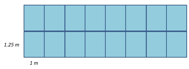
- Orientation: azimuth -9o (i.e. it is facing a few degrees East of South)
- Tilt: 35o (fixed)
- The array is assumed to be part of a larger solar installation, meaning that a similar array positioned in the front can cast shadow to our array of interest.
- Spacing between the arrays in the field is 3 m.
- Nominal array capacity 4 kW
- Assume PV cells and modules are connected in series, so partial shading along the base will affect the entire array (simplified case).
Task
Model the effect of shading on the PV array performance (kWh of energy generated) over a year. So, in the end, you will need to produce the energy output data from the array for the full-sun and shaded scenarios and observe the difference.
Directions
- SunChart. Create the Sun Chart for sun trajectory of the Baltimore, MD, location using the University of Oregon Solar Radiation Monitoring Laboratory solar tool. [66] You are to use the polar sun chart in this activity. Download your Sun Chart diagram as a PDF file. You have seen examples of this in the videos included in this Lesson. You will use this chart further to put your shading information on.
-
Apply shading. Study the “Array Packing” example in Chapter 7 of the J. Brownson’s SECS Book, understanding how shading coordinates can be obtained for a specific system geometry. Plot all the critical points by shading coordinates given in Table 7.3 on your Sun Chart. Connect the points and show the shaded zone on your diagram (see lesson videos and textbook for more guidance on how to do it). You can use a graphics software for this purpose or do it by hand if that is easier.
NOTE: the solar azimuth coordinates used by SunChart are different from those Brownson's book. The former considers 180o as true south, while the latter considers 0o as true south. So, you would need to convert the solar azimuths from the book by adding 180 in order to correctly plot the points on the SunChart. -
SAM Simulaton A (you have already downloaded SAM as instructed in Lesson 1):
- Start a new PV project in SAM – choose Detailed PV Model - Residential Owner option when initiating a project
- Under Location and Resource tab, input Baltimore, MD
- Under System Design tab, input specifications for the system (4 kW nameplate capacity, array tilt and azimuth)
- For the first round, do not include shading data
- Run the simulation by pressing the blue 'Simulate' button at the bottom left of the screen
- To get the monthly energy data in table, click on DataTables tab on top. Then choose output variables: you need Monthly Energy (KWh) and total Annual Energy (kWh) for a single year. You can also find the latter by just summing up your monthly values.
- Export your table to an Excel spreadsheet
- Sam Simulation B. Repeat the same simulation as described in Step 3 now including the shading data. This is how: Save your project as a new file. Under 'Shading Layout' tab, click 'Edit Shading' button. Then, in the editing window, choose the option ‘Enable month by hour beam irradiance shading losses’. You will be given a table to input shading factors for each hour in each month. For simplicity, we will consider the same (averaged) shading factor for all days in the same month. Looking at your Sun Chart, input 0 for no shading, 100 for full shade, and 50 for borderline or changing conditions. Once done, run the SAM simulation and export data table as described in Step 3. (See demo video in Canvas for this step)
-
Discussion. Provide a brief discussion comparing your shaded and non-shaded results and what you learned from this activity.
Submitting Your Work
Prepare a written report including the following results:
- Sun Chart for Baltimore, MD with critical points and shaded zone plotted on it.
- Table of SAM simulation results for full sun and shaded scenarios. This table should contain monthly energy generated as well as total annual energy delivered by the array. In your energy performance table, your numbers should be rounded to the nearest whole kWh (no decimals).
- Screenshot of shading factor table from SAM.
- A paragraph with a discussion of your results.
Upload your report file to the Lesson 2 Learning Activity DropBox in PDF or docx format.
Grading Criteria
- Sun Charts (10 pt). This part will be graded based on your ability to plot the calculated critical points and identify shaded versus non-shaded conditions for the system at the specific time and location.
- Energy Tables (10 pt). You will be given 1 pt per month based on the reasonable correctness of the numerical values. The purpose is not necessarily to get the exact "right" answer, but rather to have done the process and understand what you are doing. So discrepancies within +/- 30 kWh will not cause point deductions.
- Discussion (5pt).
- Screenshot of the Table with shading factors used for SAM simulation (5 pt).
Deadline
See the Canvas Calendar for specific due dates.
2.18 Summary and Final Tasks
So far, we have delved deep into the world of angles, time, and shading. Why have we done this? The solar resource is all about timing and placement of the SECS relative to the Sun, and the use of angles as coordinates in time and place are fundamental building blocks to the solar expert. We now have computational tools that make the work of calculating details trivial, but one must always know what the foundations are underneath those tools.
Who knows, maybe you will be the next open software developer to create a simple solar tool for resource assessment. You now have the keys to access many of those computational tools. More to the point, these fundamentals are not shrouded in mystery, and you don't necessarily need to pay for software to get access to them!
Looking ahead, I can tell you that students in residence at Penn State have already found a solar systems design plugin for Trimble SketchUp [68] called Skelion [69], which does shading analysis just like you performed, but on the fly inside of the SketchUp design software. Both are free to use, and I'd recommend you take a look at each in preparation for your end of semester design projects! This is an untapped resource for you to explore, now that you know "how" the shading calculations work.
Knowing these principles of angles and time also exposes us to the strengths and potential weaknesses of purely geometric relations in the solar resource. As we shall see in the next lesson, the role of the atmosphere and meteorology will tend to muck up our ideal angles of beams of light, and produce anisotropic (uneven) intensities of irradiance over the day, which will of course influence our solar resource estimations.
On to the next lesson--let's learn about the role of weather and the sky dome in estimating the solar resource!
The Goal of Solar Design and our Three New Mechanisms
The Goal of Solar Design is to:
- Maximize the solar utility
- for the client
- in a given locale.
Given the goal of solar design, we have learned of three mechanisms to leverage during the design process that will increase the solar utility for our client in their locale of interest:
- Reduce the cosine projection effect on an aperture/receiver (the extreme angles of incidence, or low glancing angles ),
- Reduce the angle of incidence on an aperture/receiver (refinement on minimizing ),
- Reduce losses from shadowing on an aperture/receiver.
In order to leverage these three tools, we have demonstrated that one needs to know where and when the Sun will be relative to our collector system.
Reminder - Complete all of the Lesson 2 tasks!
You have reached the end of Lesson 2! Double-check the to-do list on the Lesson 2 Learning Outcomes page to make sure you have completed all of the activities listed there before you begin Lesson 3.
Lesson 3 - Meteorology: the Many Facets of the Sky
3.0. Overview
Overview
This is the second of three very dense lessons on the fundamentals of solar energy. Keep it up! The lessons will lighten up a bit as we transition past these core materials.
The Sun provides us with shortwave band light at the Earth's surface, and the Earth emits longwave band light up toward the sky; but what is the role of the Sky/Atmosphere in the energy balance on Earth, and how does the atmosphere affect the bands of light that we collect and find useful at the Earth's surface? In solar energy conversion systems, engineers and design specialists apply meteorological information, particularly shortwave band irradiation (from the Sun) to inform project development and design, and also to inform daily performance of installed systems. To a lesser extent (for some radiative thermal estimations), longwave band irradiation from the Earth and atmosphere is used, but the main driver for our SECSs is the shortwave band.
Applied solar energy workers need to use the same science as those working in the field of Meteorology. The shortwave band of light can be collected via ground detectors (pyranometers/pyrheliometers [70]) or from satellites (GOES East [71], GOES West [72]) to probe and diagnose the behavior of light interacting with the atmosphere and the surfaces of Earth over time. Satellites in orbit have instruments called radiometers [73] to detect and measure the intensity (brightness) of the light scattered back to the satellite. Satellite images of visible light display the shading from clouds, the cloudiness of the Earth's surface, and features such as smoke emerging from large forest fires or volcanoes spewing ash. The signal is a measurement of electromagnetic radiation, both the intensity of the light from the Sun, and the ability of the particles or surfaces to reflect that light back up to the radiometer. Think about what determines the brightness of the light that reflects (is "back-scattered") up to the satellite.
We will start with the concept of electromagnetic radiation, including some important bands of electromagnetic radiation invisible to the human eye. We will also point out ways that a meteorologist and climatologist collect and interpret satellite or radar imagery derived from electromagnetic radiation.
As a preview to Lesson 3, please review the learning objectives on the next page to get an initial sense of the overarching goals that encompass this stage in your forecasting apprenticeship.
3.1. Learning Outcomes
At the end of this lesson, you should be able to:
- identify the seven key properties of sunlight;
- differentiate between technical air mass for lab/field-testing and meteorological air masses;
- explain the concept of climate regimes;
- apply clear sky models (REST2 or Bird Clear Sky) to a location and compare the result to real measured data;
- identify the contributions that relate to the solar resource other than the sun (clouds and ground albedo);
- explain Taylor's hypothesis and how it relates to solar intermittency (moving clouds).
What is due for Lesson 3?
This lesson has two learning activities and will there will take use two weeks to complete. Please refer to the Canvas Calendar for specific timeframes and due dates - those can vary from semester to semester. Specific directions for the assignments below can be found further within this lesson.
| Required Reading: |
J.R. Brownson, Solar Energy Conversion Systems (SECS), Chapter 3 - Laws of Light (review) C. A. Gueymard (2012) Clear-sky irradiance predictions for solar resource mapping and large-scale applications: Improved validation methodology and detailed performance analysis of 18 broadband radiative models [74] Solar Energy 86, 2145-2169. |
|---|---|
| Optional Reading (not required): | Bird and Hulstrom (1981): Simplified Clear Sky Model for Direct and Diffuse Insolation on Horizontal Surfaces, Technical Report No. SERI/TR-642-761, Golden, CO: Solar Energy Research Institute Meteorology for Scientists and Engineers, 2nd ed. by Roland B. Stull (Chapter 7). J.R. Brownson, Solar Energy Conversion Systems (SECS), Chapter 8 - Measure and Estimation of the Solar Resource |
| To Do | Learning Activities
Discussion: Climate Regimes Quiz Assignment (See Canvas) - due by the end of the first week Engage in all Try-This and Self-check activities included in the lesson (not graded). |
| Topic(s) | Principles of Light behavior Engineering Air Mass Meteorological Air Masses Clear Sky Models Anisotropy from clear and non-clear sky (and ground) Clouds and solar intermittency |
Questions?
If you have any questions, please post them to the Lesson 3 General Questions and Comments Discussion Forum in Canvas. I will check these forums regularly to respond. Feel free to go through the comments and post your own responses if you are able to help out a classmate.
3.2. Basic Rules of Light Quantification
Reading Assignment
- J.R. Brownson, Solar Energy Conversion Systems (SECS), Chapter 3: Laws of Light.
While reading, pay attention to the basic rules of light measurement. Our historical affinity for burning fuels has been paired with an affinity and strong awareness of temperature, but we lack an awareness for measures of light, found through radiometry. Think of how you “know” what 80 °F versus 65 °F means. Why not measure the irradiance/irradiation along with the temperature? What if we, as a solar culture, were to learn what 1200 W/m2 meant versus 500 W/m2 for an average hourly or minute irradiation upon an exposed surface (vertical wall or sloped rooftop)?
Radiometry
For solar resource assessment, radiometry (the measure of electromagnetic or radiant energy) is more valuable than thermometry (the measure of temperature). Solar energy is comprised of the shortwave band of light found between 250-2500 nanometer wavelengths of light ( , or one billionth of a meter). Within the solar field, we measure the shortwave band in terms of irradiance, as W/m2 (Watts per square meter, a flux of light per receiving area). If we group irradiance over a block of time, say an hour, we call the measure irradiation, in units of Wh/m2 (Watt-hours per area, similar units to electrical energy measure).
Quick Terms and Concepts:
- Radiometry: measure of radiant energy
- Shortwave: solar band of interest in measurement for the applied solar field
- Nanometer: wavelength units for light/photons (sometimes micrometer)
- Electron volt: energy unit for light/photon wavelengths ( )
- Irradiance: metric for flux of light received on a surface (W/m2)
- Irradiation: solar field convention, metric for energy (Wh/m2 Watt-hours per area or Joules per area)
- Photometry: measure of optically perceived light (illuminance, illumination). Photometry is not used for solar resource assessment.
Technical Shortcut:
To convert energy values as electron volts from nanometer wavelengths: divide 1239.8 nm•eV by the wavelengths that you found in nanometers to find their respective energies in electron volts (eV). Because the error is negligible for us in the field, we can even use 1234.5 nm•eV (just count to five and use the right decimal point).
For more information on how we get to this equation, see the Key Equations [76] page in the Resources box.
Traditional silicon photovoltaics collect energy for electricity production from wavelengths <1100 nm. Other systems like solar hot water panels will collect almost all of the spectrum from the Sun. In fact, almost all of the opaque surfaces about our environment (buildings, roads, water) tend to absorb strongly over the entire shortwave range (leading to an increase in temperature!).
And yet, our wonderfully adaptive human eyes only capture the tiny visible band from 380-780 nm. Thanks to the complex feedback systems from our irises, lenses, and eyelids, eyes can adapt well to extreme conditions of bright or dim lighting but cannot be used to quantitatively gauge irradiance conditions that energetically drive our buildings and photovoltaic systems. Our eyes impart important information, but because they are highly sensitive and adaptive systems, our eyes cannot be used to reliably distinguish and evaluate the solar resource (bare skin may actually be a better receptor for the shortwave band on days that are not windy).
Notice that the "visibility" of a photon is really limited only by the type of detector being used. Let's review the distribution of photons across the electromagnetic spectrum, and then we will discuss types of photon detectors beyond the rods and cones in our eyes. As a reminder, 1 micrometer wavelengths (also called 1 micron wavelengths) are equivalent to 1000 nanometer wavelengths (by unit conversion). It is often easier to use units of nanometers (nm) for the shortwave band, while using units of micrometers (um) for the longwave band. Either will work, but it is helpful to be aware of the relationship.
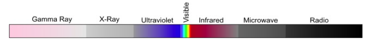
Diagram of the broad possible spectrum of electromagnetic radiation from left to right: Gamma Ray, X-Ray, Ultraviolet, Visible (small section), Infrared, Microwave, Radio
Now, let's zoom in to the shortwave and longwave bands important to SECSs. Wavelengths are expressed either in nanometers (nm) or micrometers ($\mu m$, also called microns). For wavelengths greater than 380 nm, electromagnetic radiation transitions from the ultraviolet (UV) to the violet visible range for the human eye. As we will observe in the Granqvist figure below, the red visible range ends for wavelengths greater than 780 nm (to the human eye). Notice how the "infrared" crosses over both the shortwave and longwave bands of light.
- SECS have a different operational "grouping" of bands than traditional spectroscopy or remote sensing. Get used to shortwave and longwave bands, as we describe below.
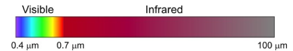
Video: Temperature and Wavelengths (0:57)
Let’s explore a simple model of how oscillation frequency is tied to the wavelength of electromagnetic radiation.
The frequency at which electrons oscillate is essentially set by the temperature of the matter in which the electron resides. Lower temperatures yield lower frequencies of oscillation. Here, we’ve set our temperature on the low side, and you can see the molecule oscillating fairly slowly, or in other words, at a low frequency. The wavelength of the emitted radiation is also relatively long.
But, when temperature increases, the oscillations get faster, which makes for a higher oscillation frequency. This high frequency means that the emitted electromagnetic radiation has a relatively short wavelength. For comparison again, we can decrease our temperature to watch the oscillation frequency slow, and the wavelength of the emitted radiation increase.
All objects glow with energy in proportion to temperature. As temperatures increase, the wavelength oscillations become shorter and the density of photons measured is effectively increased. So, the light becomes more intense (more photons), and each photon is packed with more energy.
Most photons are emitted from a thermal surface, where the constituent atoms are vibrating in the material (this means: temperature). Every material has a thermal property, and hence "everything glows." This concept works well for something called "blackbody emission" (zero emittance) or "greybody emission" (non-zero emittance) but not so well to describe your standard laser pointer or microwave oven. So, just to clarify all cases, there are also photons emitted from the Sun and from solid state devices that are "stimulated emission" (lasers), which can allow for photon emission from surfaces that are high in energy, but not high in thermal temperature.
First rule of Solar Energy: Light is Directional.
This is our first principle of seven for the behavior of light. So, let's begin with the simple yet important statement: Light is directional. Light, as a photon, is born (emitted) from a surface in many directions and then impinges upon other surfaces, where it is either absorbed, reflected, or transmitted (and refracted). We use that directionality to describe the resource. In the text chapter, we have defined a visual shorthand for light that is emitted, transmitted, reflected (scattered), and/or absorbed by various surfaces.
- Irradiance (W/m2): light that impinges upon a receiver surface, interpreted as the instantaneous rate of change in energy (called power, or Watts) per unit area. Remember that one Watt is equivalent to one Joule per second (a rate of energy exchange).
- Irradiation ($J/m^2$ or Wh/m2): light that impinges upon a receiver surface over a period of time, interpreted as the energy (in Joules or Watt-hours) per unit area.
- Radiance (W/m2/sr): light emitted from a surface, interpreted as the instantaneous rate of change in energy (call power, or Watts) per unit area per steradian (a unit of solid angle). If we were to generalize radiance over all exiting directions or angles ($W/m^2$), we term the energy emittance as radiant exitance.
- Radiation (J/m2 or Wh/m2): here, using the convention of the field, radiation means light emitted from a surface over a period of time, interpreted as the energy (in Joules or Watt-hours) per unit area. This is a loose operational definition, as "radiation" can mean many different things to different fields of study.
Notice that the "Ir-" instructs us that the light is incident upon a surface. For example, we measure "irradiance" on a pyranometer, because light is absorbed by the device. Also, notice that my choice of "-iance" or "-iation" determines if the light is a measure of rate (as in power: energy per time) or energy (rate integrated over a span of time).
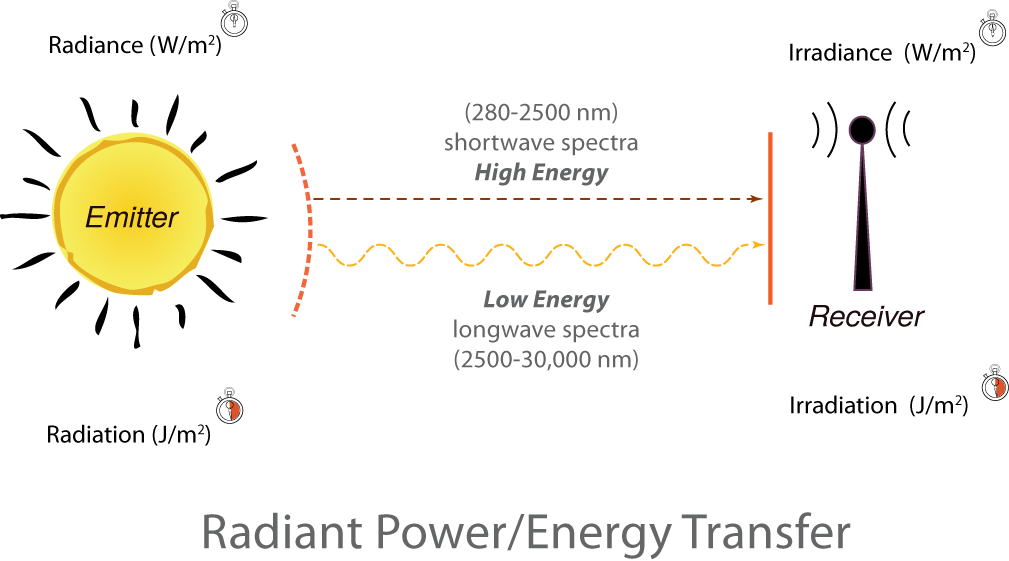
Left to right:
Left: An image of the sun is labeled Emitter. Above the sun is the label: Radiance (W/m2) and the image of a stopwatch. Below the sun is the label: Radiation (J/ m2) and the image of a stopwatch with the right half filled in.
Proceeding to the right: Two lines from the sun travel to a Receiver on the right. The top line is a straight dotted line labeled (280-2500nm) shortwave spectra High Energy. The second line is a wavy dotted line labeled Low Energy longwave spectra (2500-30,000 nm)
Right: Above the Receiver is the label: Irradiance (W/m2) and the image of a stopwatch. Below the receiver is the label: Irradiation (J/ m2) and the image of a stopwatch with the right half filled in.
Second Rule of Solar Energy: Light is Spectral.
All objects glow (even the gases in the sky); it is just the intensity and peak wavelength that shifts with respect to their thermal temperature. This brings us to the second of the seven principles of light behavior. Light (e.g., derived from the sun) has a broad spectrum of energies, which are discussed as wavelengths. We tend to group similar wavelengths in the spectrum according to the properties of their emitting surface or receiving surface.
Short Wave Band (250-2500 or 3000 nm)
This is a "group" of high-energy wavelengths of light that are emitted from the Sun (See Light is Directional), comprising the majority of the total energy collected by the Earth's surface or our designed SECS, given the decrease in the light power density with distance to Earth (93 million miles, 150 million km). This bundle of wavelengths of light emitted from the sun includes the ultraviolet (UV), the visible, and the near infrared (IR) sub-bands.
- Shortwave band: The shortwave band of wavelengths is confined from approximately 250 nm to 2500 nm at Earth's surface, because of the Inverse Square Law [77] for light and the nature of our atmosphere as an absorber/reflector of longwave irradiation. Our measurement devices are also limited to measuring this range by the transparency of low-Fe glass covers.
The Sun is effectively the only surface from our surrounding environment that regularly and naturally emits shortwave radiance. We can deliver shortwave band energy to a new surface using a reflector, though, as is the purpose of light concentration onto a central receiver.
Long Wave Band (2500 or 3000 nm - 50,0000 nm)
Long wave band consists of low energy light. The wavelengths of light that are emitted from our skin, from pavement, the sky, ice cubes, and even hot ovens are coming from surfaces that are quite cool relative to the surface of the Sun, right? We are comparing 250-500K surfaces to a 6000K surface. Planck's Law (discussed in the next page) suggests that the distribution of wavelengths will be very different from cool bodies than from extraterrestrial bodies with internal fusion reactors.
The group of wavelengths from cool bodies on Earth is termed the longwave band. This is >2500nm at Earth's surface, but also can be >3000nm if we were to group the wavelengths from space. The longwave band photons are of lower energy, but there is a very wide band of wavelengths included in the group. The longwave band contributes to the greenhouse effect, and keeps our atmosphere comfortably warm. With the addition of CO2 and water vapor to the atmosphere, we make the sky into a better reflector for keeping longwave energy instead of allowing it to escape into space.
- Longwave band: The longwave wavelengths are found in the range of 2500 nm to wavelengths greater than 50,000 nm, and again our measurement devices are limited to the range of about 30 or 50,000 nm. This second "group" of wavelengths of light is emitted by surfaces significantly cooler than the Sun! This includes the surface of our human bodies, the surface of Earth, and the effective surfaces of Earth's atmosphere (if we were to simplify the atmosphere to two surfaces in a slice of gas and particles).
Now, we're going to take a moment to explore the following multiple figure graphic from Smith and Granqvist. There is a lot of information in here, so take your time and revisit it as the class progresses.
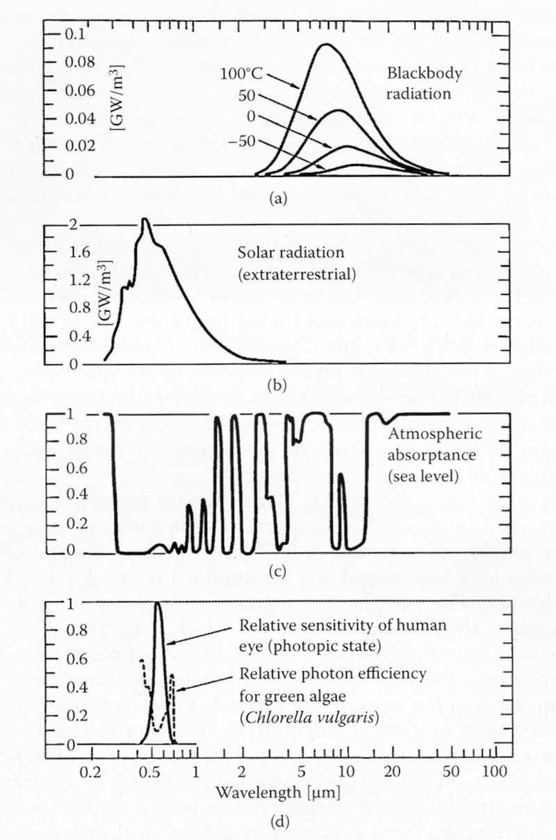
- The top graphic, Figure (a), shows the longwave spectrum of radiance (remember, that means "emitted power") from any surface at "ambient" Earth temperatures (-50C to +150C). You see a series of four humped curves that get more intense (bigger), while the peak shifts toward the left (higher energy) as hypothetical surface temperatures increase from -50C to +100C. These temperatures include the Earth's atmosphere, your body, the interior walls of your homes, even a glacier. Remember, all surfaces "glow." This spectral region is the Near-, Mid-, and Far-Infrared, and you may have seen false color images of these emitted surfaces from IR cameras before. The irradiance scales are from 0 to 0.1 W/m2/nm.
- Next, Figure (b) shows the spectrum of Solar light measured just above the atmosphere. The intensity of solar irradiance (remember, that means "received power") at the atmosphere is reduced in proportion to the inverse square of the distance from Sun to Earth. There is effectively only one temperature for the surface of the Sun, and so only one curve, which is far to the left relative to the curves in Figure (a). Also, notice that the intensity of the curve is significantly greater, with a scale from 0 to 2 W/m2/nm.
- Figure (c) shows spectral regions where shortwave and longwave radiation passes through the atmosphere. This is an absorptance spectrum; so, areas where the curve is near one (e.g., 4-8 micrometers) completely absorb the outgoing longwave from Earth and the surrounding atmosphere. Areas where the curve is near zero (e.g., 8-13 micrometers) will allow longwave light to transmit into outer space. The gap between 8-13 micrometers (8,000-13,000 nm) is called the atmospheric window, or the sky window, where the molecules CO2 and H2O do not absorb or reflect, and through which a portion of the longwave band can escape. Soon, we will design terrestrial emitters to selectively send energy out the window. This is where longwave radiation from the Earth and Atmosphere leaks radiant energy out into space. Compare Figure (c) with Figure (a) and notice how much they overlap each other.
- Finally, Figure (d) shows a solid line with a peak near 550 nm, demonstrating the relatively tiny region of sensitivity of the eye for detecting photons under daylight conditions (called the photopic state). This is a pretty small energy band, and does not include the behavior of the iris, the eyelids, and the direction your eyes are pointing with respect to your eye lenses. The double peaked dashed line (around 420 nm and 700 nm) is the efficiency of light absorption for green algae, again confined to a tiny region of the whole spectrum. Both curves are normalized fractional scales from 0-1.
Third Rule of Solar Energy: Inverse Square Law
Light intensity decreases in proportion to the square of the distance between emitter and receiver. This is called the Inverse Square Law, which applies to solar energy as well as to any other light source. In case of the Sun, the emitted energy flux is 6.33x10⁷ W/m2 at the surface of the Sun drops down to 9126 W/m2 at the surface of Mercury (d=58 million km), and down to 1361 W/m2 at the exterior of Earth's atmosphere (d=150 million km).
As shown in the next figure, the reason for the inverse square law is geometric in nature. As light is emitted from a point, like the Sun at a very large distance, the same quantity of photons is spread out over an increasingly larger area with distance. Area is a spatial term in units of distance squared. This same principle works for ordinary surfaces, as photographers well know.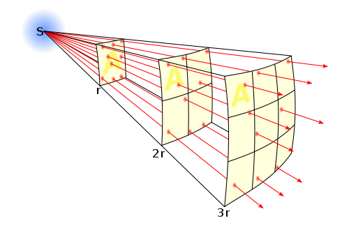
Mathematically, this process of light “dilution” can be represented by the following equation (which is another form of Equation 3.2 in the SECS textbook)
\[G_2^{} = {G_1}\left( {\frac{{d_1^2}}{{d_2^2}}} \right)\]where G1 is the light intensity (or flux) at distance d1, and G2 is the light intensity at distance d2.
If we take G1 as the radiative energy flux at the surface of the Sun, we can then estimate the radiative energy flux at the Earth’s orbit (G2) using this equation simply based on the planetary distances. Try to make this calculation with d1 being the Sun’s radius, and d2 being the distance from the Sun to the Earth and see what you get. You will have a chance to share your result in the Lesson 3 Activity further in this lesson.
Self-Check
3.3. Four Laws of Light
Reading Asignment
- J.R. Brownson, Solar Energy Conversion Systems (SECS), Chapter 3: Laws of Light
We continue our review of the seven basic rules, or "laws," of light. These four are a bit closer to physical laws than what's on the prior page, but we need to understand the basics of light if we are to move on to the physics of light interacting with the atmosphere.
You may want to use the math/science site Wolfram Alpha [79] to solve several of these Self-Test questions quickly, or to check some of the notes in Wolfram Alpha against our own work here. Wolfram Alpha is the Google of math and physics. If you want to do calculations on Wien's Law, you type "wien's law" and you will get a calculator for Wien's Law with all sorts of other information.
Kirchoff's Law
This radiative transfer law is very important when considering energy balance. It states that at thermal equilibrium, the emissivity () of a body or surface equals its absorptivity ().
Mathematically, we can conceptualize Kirchoff's law as
The radiant energy emitted from a real surface is represented as E (W/m2), while that of a blackbody (a theoretical condition) is given by EB (W/m2).
Simply put, a surface at steady state temperature will absorb light equally, as well as it emits light. Though light is directional, surfaces exchange photons in both directions.
Planck's Law
This law is generalized to mean that all objects have some internal temperature, and given that temperature, they all glow. Max Planck was able to establish the dependence of the spectral emissive energy of a blackbody for all wavelengths of light (), given a known equilibrium temperature of the blackbody.
Wien's Displacement Law
The Wien's displacement law provides us with expected values for the most probable wavelengths in the Bose-Einstein distribution of blackbody radiation. The law implies that the distribution of photons emitted from a surface at any temperature will have the same form or shape as a distribution of photons emitted from a surface at any other temperature. Mathematically,
Stefan-Boltzmann Law
The Stefan-Boltzmann Law states that the radiative energy emitted by a surface is proportional to the fourth power of the surface's absolute temperature. The Stefan-Boltzmann Law shows that if you were to integrate all the energies from the wavelengths in Planck's Law, you have an analytical solution of the form below:
where = Stefan-Boltzmann constant
Keep in mind that this is for the surface of the emitter. A surface like the Sun will have a very high value for the energy density on the surface, which then decreases in proportion with the Inverse Square Law from the last page (over the 93 million miles distance to Earth's surface).
Self-Check
3.4. Learning Activity: Laws of Light
Wolfram Alpha website [80] is the Google of math and physics. If you want to do calculations on Wien's Law, you type "wien's law" and you will get a calculator for Wien's Law with all sorts of other information. The purpose of this activity is to practice some basic calculations of physical properties of sunlight.
Short Problems:
- Use Wolfram Alpha [79] to calculate the most probable wavelengths emitted by the surface of the Earth (T=300 K) and the Sun (T=5778 K) using one or more of the laws discussed on the previous page of this lesson. What is the meaning of the "most probable wavelength"?
- Use Wolfram Alpha [79] to calculate the energy flux (radiant exitance) emitted by those Earth's and Sun's surfaces using Stefan-Boltzmann Law.
- Apply the Inverse Square Law (see formula on page 3.2 of this lesson) to determine the "extraterrestrial solar flux" at the Earth using the Sun's radiant exitance found in Question 2.
- Discuss the meaning of "extraterrestrial solar flux" and how it is further transformed within the Earth's atmosphere.
This video below (6 min) presents a short demo on how to use the Wolfram Alpha site. The Stefan-Boltzmann Law is used as an example here, so it provides you with a tip for solving the second problem.
Submitting Your Work
Prepare a written report with your solutions and upload it to Canvas (Lesson 3 Learning Activity Dropbox) in PDF or docx format. You can use Wolfram Alpha screen shots to present your results for the first two problems (insert the screenshots into your report - don't submit them as separate files). Make sure to present the equations you are using and provide comments to the steps in your solutions.
Grading Criteria
View the Rubric in Canvas by which this assignment will be graded.
Deadline
See the Calendar tab in Canvas for specific due dates.
3.5. The "Life" of a Photon
Reading Assignment
- SECS, Chapter 3: Laws of Light, beginning sections through "Light is Directional"
Remember how we stated that light is directional? Light also has a "life" including the birth and death of a photon. Electromagnetic radiation is emitted from a surface and will encounter objects in its many paths. The fate of electromagnetic radiation (as a photon) depends on wavelength of the photon at hand and the physical composition of the objects along its path. Again, the photon is a packet of radiation and can interact with molecules or atoms in its path, being transmitted, absorbed, or reflected.
The action of "reflection" is more appropriately described as "back-scattering" by atmospheric physics, which is why you see that term in the figure of possible paths of light. We also have seen a shorthand diagramming technique from the textbook to describe the life events of ensembles (really big groups) of shortwave and longwave photons.
I would like to pull the concept of photon lifetimes in the following video.
Video: Diagramming Light Intro (2:03)
All right, so let's do a quick discussion of the sources of radiation, source of light, and the surfaces that receive light in the lifetime of the photon, right?
We know that from our little diagram technique, that source of light we diagram as a curved surface. We can diagram a straight arrow that's going to signify shortwave band light. We could draw a curvy arrow line that's going to signify a longwave light.
So, right now, we've got what is going to be a black body emitter that is emitting both shortwave light and longwave lights which probably have a pretty high temperature surface, something like the sun, maybe around 6,000K. And it's going to emit light, it's going to travel a long distance.
Somewhere along the distance, it's going to be transmitted through a transparent surface, something like maybe a window, the atmosphere. And, ultimately, it's going to meet its end where it will be absorbed by some opaque surface. We're going to have something dark and opaque over here that's going to absorb the light. And I've got these little dashed lines to signify absorbed light.
However, if that material were heading in, say, it went through the window again, and were to hit a reflective material, something like a mirrored surface. We would draw that light bouncing off the surface, and, of course, it would not be absorbed by the surface. In reality, we have surfaces that do both things, that absorb some of the light, and reflect some of the light.
We're going to have-- use the symbol rho for reflectance. Maybe it is reflecting 30% of the light and it is absorbing 70% of the light. We would give these fractions from 0 to 1 to describe those percentages. But we certainly can do that in a quick diagramming technique.
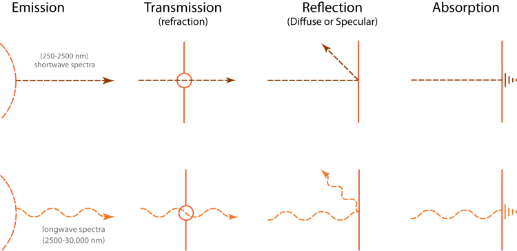
Each of these phenomena is happening simultaneously, and the next video opens up that discussion.
Video: Light Interactions Descriptive (4:31)
So, right now, you're looking at an image in the website. It's really diagramming everything that can happen when light is interacting with matter, with surfaces, with molecules, what happens in that process in the lifetime of a photon. And what I like about this diagram is it's actually diagramming everything happening at once, which is more realistic of what's actually happening.
Remember that when we say incident radiation, what we're talking about-- light is directional-- and so we have a language for light that's being emitted from surfaces. That's radiant exitance, radiance, radiation. And we have the language, the terminology for the light that is incident upon a surface. And so, what we would call this-- we probably correct this to call this irradiance, N-C-E, or irradiation, as well. So, either one of these is talking about light incident upon a surface.
And so, again, what we're seeing is light coming into a surface. This is really meant to be indicative of what's happening in the atmosphere. And so, we have light that is absorbed by this material, and this could be the atmosphere or it could be clouds. It could be water molecules, for that matter. We have scattering happening in, and the scattering events are basically reflections. So, back-scattering is really indicating reflection. Absorption is indicated by alpha. So, we have scattering events on a surface, even though that surface, in our case, is a single dot. And the scattering, in our case, could be back-scattering. It could also be forward scattering happening. And that's why you had these two different arrows.
And the last that you have is transmission, and that's really that nothing was absorbed. So we're going to diagram that with a circle. That's going to be a tau equal to or, let's say, a tau approaching one. Something that is very transparent is going to have a coefficient, a fractional value closer to one. Something that is very dark, very opaque is going to have a fractional value close to one for alpha.
And somewhere in between this, all of these things happening, we have to recognize that all this light coming in is going to be equal to one in a fractional sense. And then, the three different things that can be happening is it could be absorbed, it could be reflected, and it could be transmitted. But the balance of all of that energy is still going to add up back into one. So, we can have a very opaque material, which will have a high absorption coefficient, and transparency that will go towards zero, in which case we'll have, basically, just absorption and reflection happening.
And that reflection and absorption process happening is called a gray body. So, it's an opaque material that reflects some of the light and absorbs the rest of light that is incident upon that surface. And if you think about it, when we want to call something a black body, what a black body means is that the absorption is all one. It's absorbing perfectly. It's not reflecting any of that light. It's not transmitting any of that light. That is a black body. And a black body, like the sun, which is a very close approximation of a black body, is also going to use Kirchhoff's law, so you'll have absorption equal to emittance, and so the emittance is going to be equal to one as well.
So, we've got some pretty interesting stuff going on that's really demonstrating everything that we've learned about light so far, and we've demonstrated that we've got a few diagramming techniques that will tie this together.
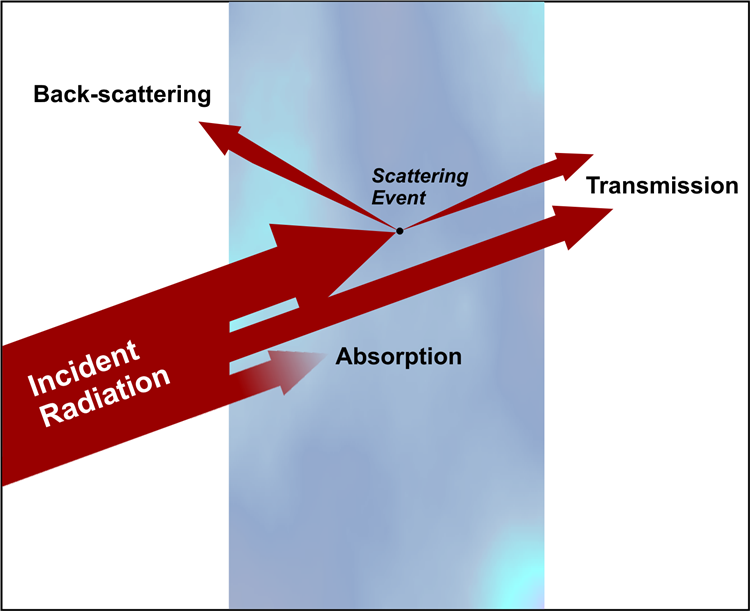
Emission ($\epsilon$), absorption ($\alpha$), reflection ($\rho$), and transmission ($\tau$) can all occur at the same time (in fact it always does). We also know that there is a relationship between light energy balances and temperature. When a receiving surface or material absorbs more energy than it emits, the internal temperature of the material will increase (effectively pumping up the system's energy density). Consider a bright summer day, where your rooftop absorbs much more solar radiation than it emits (or conducts away). The roof surface temperature will rise from just after sunrise to the late afternoon.
Video: Light Diagramming Example (5:49)
Now, let's put our diagramming into action. So, we've already learned our shorthand that the surface emitting light is going to have a curved arc. So, light coming out of that surface is short wave. It's going to be a straight line from a different surface. This is going to be some surface at temperature one.
A different lower temperature surface is potentially a very good long wave emitter also having a curved arc for the emitting surface and a wiggly line, in this case, that signifies that long wave band. That's that band greater than 3,000, 3,000 to 50,000 or 3,000 to 30,000 nanometers, whereas the short wave is a 250 to 2,500 nanometer range.
Any other notations we're going to come across here in just a second, but you can see here I've got a diagram of the sky dome. This is pretty common arc that we're going to have in the class. Just saying, look, there's this entire sky here, and it in and of itself is going to be a source of light. How do we diagram that?
Well, first, let's put a receiving surface on the ground. We'll say that we have a solar panel on the ground here, and it's going to be a receiver of light. And so, I'm going to now start diagramming.
I know that the sun is a source of emission of light. That's going to be short wave light. Short wave light, as we will see in just a second, is effectively transparent to the atmosphere. So, it's passing straight through the atmosphere without being absorbed.
And, ultimately, it's going to come to the surface. A portion of it might reflect off. The rest of that light is going to be absorbed by our solar reflector and thus generating the excited states for electrons if it's a photovoltaic panel, hot water if it's a solar hot water system. But that's our main source of energy that we think of, and that's that beam component of light that we'll talk about eventually.
There are other sources of light in this system, and we want to diagram them. So, for example, we know that the sun will hit the ground and it will reflect off the ground. We're going to have a lot of light that's coming and hitting the ground and reflecting off of it. And that reflected light off of the ground is called the albedo. But, in our case, we're just diagramming it as a check mark on here, and it will ultimately also be a secondary, but a source of light for this tilted panel. That's the participation of the ground in the short wave energy.
The sky itself is full of back scattering. We had this diagram of forward scattering and back scattering across the atmosphere. I'm going to diagram all of that as straight lines coming off of the surface of the sky dome with the idea that all of this light is still reflected light. It's still scattered light. It's not emitted light, otherwise, I would have a curved surface here, but I don't. I've got just a straight line showing that, basically, this is all reflected light.
And so, this is a diffuse reflected light source for our solar panel, just as the ground is a diffuse reflected light source as well. All of these together are short wave component sources of light for our solar energy conversion system.
Now, the ground and the solar panel are each going to also have their own thermal characteristics. Everything glows. This is one of the principles of light is that ultimately, everything's going to glow, and it's all going to have some light characteristic to it. In our case, it's going to be the ground and the panels emitting long wave light.
So, these guys are emitting long wave light upward into the atmosphere. The atmosphere itself has a temperature. It has an ambient temperature. All those gases have a temperature, and so those gases are going to emit as well, both down to the ground and up out into space.
And so, we have actually pretty well diagrammed a lot of the major energy balances of light, just using this simple notation. You can see that the temperature of the ground is going to be one source of long wave. The temperature of the solar energy conversion system is going to be another source. The temperature of the atmosphere is another source, and of course, the temperature of the sun is the source of our short wave light.
And we know the sun is approximated by a black body at about 5,777 Kelvin, whereas all of our terrestrial surfaces are going to be somewhere in the order of 300 Kelvin. Much, much lower than the temperature of the sun. And yet, you can see that we have a great way to do some quick diagramming to hopefully understand--
Recapping: Electromagnetic radiation (as light) is first emitted, and the emitted photons have an opportunity to be transmitted, absorbed, or reflected by an intervening surface. If that surface is a particle or an assemblage of particles, there will be a tendency for the reflection to be more accurately described as "back-scattering."
In solar energy resource assessment, clouds are the most important atmospheric factor influencing device performance, followed by aerosols (dispersed atmospheric particles).
3.6. Case Study: The Atmosphere as a Selective Cover
Reading Assignment
- SECS, Chapter 5--Meteorology: the Many Facets of the Sky (section on Air Masses)
Case Goal: Develop a working concept of the atmosphere as a case study of a selective surface, interacting in concert with the Earth surface to contribute to the global energy budget. Then, move on to more specific reflective surfaces that we might use as a secondary shortwave resource (diffuse reflectors and specular reflectors) in designing SECS.
The Earth is a vast solar energy conversion system! The atmosphere encasing Earth's land and water mass is a collection of gases and particles that vary in pressure, temperature, and chemistry continuously. If we collectively imagine for just a moment that the atmosphere is a simple cover on top of our main absorber (the Earth), we can begin forming a concept of the atmosphere interacting with electromagnetic radiation across broad bands of wavelengths.
Now, let us consider the optical properties of a single material that reflects light for some bands and transmits or absorbs light for alternate bands, just like the atmosphere represented above. We call the surface of such a material a selective surface, because the light interaction occurs at the surface. A selective surface is non-reflective to some bands of light, while being reflective to other bands of light. The atmosphere is a case study for a selective covering surface between shortwave and longwave bands.
For any given wavelength or band of similar wavelengths, the following three simple phenomena will occur when light interacts with a material surface (where light is either being absorbed or emitted):
This means that each of the simple optical phenomena can be represented by fractions from 0 to 1, with the sum of these equating to 1.
For opaque materials, there is a relation between reflectivity and emissivity (the glow of an object) and between reflectivity and absorptivity.
- A surface that is highly reflective for a certain band of wavelengths is also a surface with a low emissivity.
- Meaning: reflective materials don't 'glow' effectively.
- In contrast, a surface that has low reflectivity for certain wavelengths of light will have a high emissivity.
- Meaning: non-reflective materials tend to 'glow' effectively.
We now know the relation for surfaces in optics called Kirchoff's Law of Radiation. When a surface is in thermal equilibrium with the surroundings, the emissivity is equal to its absorptivity at each wavelength ($\epsilon = \alpha$). This allows us to make the same relations among reflectivities and absorptivities.
- A surface that is highly reflective for a certain band of wavelengths is also a surface with a low absorptivity.
- Meaning: reflective materials don't absorb light effectively either.
- In contrast, a surface that has low reflectivity for certain wavelengths of light will have a high absorptivity.
- Meaning: non-reflective materials really do absorb light effectively.
We can show the ways in which the Earth-Atmosphere is selective in the relative properties of each to absorb, reflect, and transmit different bands of light.
Video: Solar Case Study (6:47)
Starting again with the image of the sun interacting with the atmosphere and the Earth. The atmosphere is a cover. It's a transparent cover relative to some wavelengths. And we'd like to use that as our quick diagram and case study.
So, we've got the sun that is emitting shortwave light. It is transparent in the shortwave, for the large part. That sunlight ultimately interacts with the Earth's surface, where it is absorbed. A portion of it is absorbed. And a portion of that light is reflected. And that reflected light ultimately is going to leave the atmosphere.
What we find out is that that amount of light that's leaving the atmosphere, whether it's reflected off the ground, or let's say, for example, it's sunlight that is being reflected off of clouds. We're still assessing that these (total) are going to be on the order of 70% to 75% of light. And that would be evaluated with a row of 0.7. We'd have-- from the balance, because the Earth is opaque, we'd have an alpha value of 0.3, so alpha of 0.3 for the surface of the Earth. That would make the transparency approximately 1 for the Earth's atmosphere.
Now that's part of the balance, and that's all the shortwave. But the Earth itself in this case study, again, has a given temperature. The temperature of the sun, and the temperature of the Earth, and the temperature of the atmosphere are all going to come to play in this.
Shortwave is coming from the source of the sun, because the sun's surface temperature is that 5,777 degrees Kelvin, or approximated as such. And the Earth is going to be emitting longwave light. The atmosphere is going to be emitting longwave light, only the atmosphere is actually two surfaces-- a top surface and, effectively, a bottom surface, and will be emitting up and down longwave radiation.
However, the Earth itself-- let's grab this guy and simplify it again-- the Earth itself is going to be emitting this longwave light. And a large part of that longwave light is going to be absorbed by the atmosphere. Some of that light, however, emitted by the Earth, is going to make its way through the atmosphere, and it's going to have a very low transparency-- we'll say approximately 0.1-- but some of that makes its way out.
And it makes its way out through what we call the sky window, or the atmospheric window. And that sky window is occurring in a specific band-- this is a selective surface of its own anywhere from 8 to 13 micrometers. We have a gap, a leaky window, where longwave radiation can escape.
So, if I went to grab this image that we've been looking at before, you're going to see a range, and we're going to dial into where is that sky window happening? So, somewhere right in here is a range that's lining up over in this area. And that range, if we look closely, is going to be-- let's bring that down here and carry that down.
That's going to be at about 10, 9, 8 nanometers. And the next one is going to be right here. Let's grab that guy. And he is going to be at out-- that's about 20, so half of that's 15, and approximately right there is about 13 or 14 micrometers.
So, again, from 8 to 13 micrometers, we have in this range right here and here, is our window where we're getting a percentage, actually, that looks like a higher percentage-- 15% to 30% of light transmitted through the Earth's atmosphere. On this side over here, we see that whole spectrum that is the solar spectrum from the sun. And it's in the small percentage in the UV, a bigger percentage in the visible band, and a very large percentage of light that's coming through the atmosphere that is in the infrared band. But ultimately, it all cuts off at about 1, 2, 3,000 nanometers. And actually, if we were to look closely, the atmosphere actually cuts off at about 2,500 nanometers.
Now, the other thing that we can look at in this diagram is, what are the sources of the walls of this atmosphere? I draw that arrow down-- oops-- if I draw that arrow down, I see that one of the absorbing gases is carbon dioxide. And on the other side of this, the main absorbing gas is going to be water vapor, water vapor and oxygen.
So, essentially, I have water vapor on this side. I have CO2 on this side, that are limiting the leakiness of the atmosphere to lose energy, to leak energy into space. And that's actually the valve mechanism that we'd tie into the greenhouse effect. So, if you increase CO2, you start moving the valve tighter. You heat up the atmosphere, you increase the water content, you squeeze things a little tighter. And you actually lose your leakiness, and you drive the atmosphere more and more warm.
OK, that's the end of our case study. Let's move on to the next.
We have already described shortwave (280-2500 nm at ground level) and longwave (>2500 nm) bands of irradiation incident upon a surface. The study of optics is that of light-matter interactions, regardless of wavelength. We know that materials like glass are semi-transparent in most of the shortwave band, and materials like pure aluminum are reflective in the shortwave band. We are not so familiar with the way that materials behave in the longwave band, and we often have trouble with materials that are opaque vs. semi-transparent.
Let's review the transmittance graphic that I introduced earlier. This plot has a logarithmic x-axis, so, we can count from 0.2 micrometers (200 nm) up to 1 micrometer wavelengths in increments of 0.1 micrometer. Then, we count from 1 micrometer to 10 micrometers in increments of 1 micrometer, and so on...
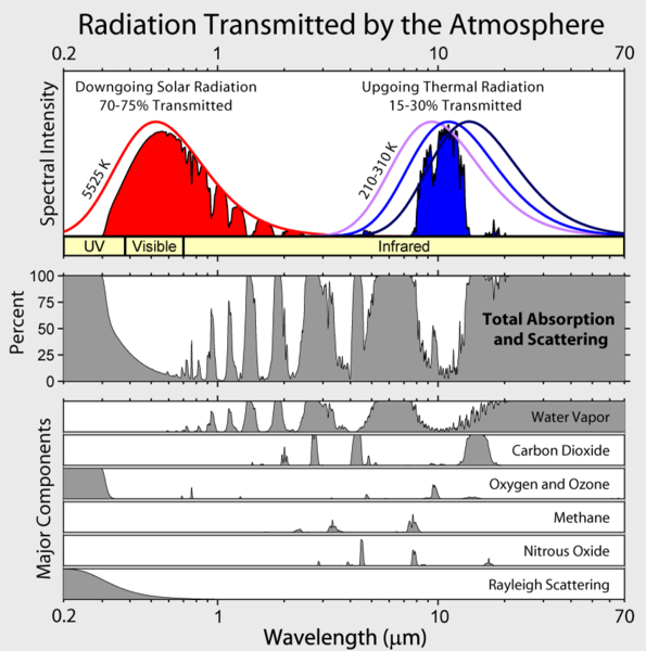
We see that from about 0.3 micrometers to about 2.5 micrometers, there is a significant amount of white showing on the plot of the Total Absorption and Scattering, meaning that the absorption and reflection of visible light by the atmosphere is relatively small. In other words, the atmosphere transmits 70-75% of the sun's shortwave light from the top down to the Earth's surface. Along the way, clouds can back-scatter [82] (reflect) some of the visible light into space. In times and places where transmitted sunlight reaches the Earth's surface, then the land, oceans, deserts, grasses, and trees, etc., reflect some of the surface-incident shortwave light back into space (again, with limited absorption along the way).
We also see that from 8-13 micrometers, there is an atmospheric window where the longwave band light is not absorbed or scattered. This is the way that the Earth and the Atmosphere can "leak" energy back into space. If you like, go back to take a look at a similar figure from Granqvist. From which side of the sky window is water vapor absorbing the longwave light, and from which side is CO2?
Using this example, when incident light (irradiance) is not absorbed or transmitted through the surface and bulk of a material, it is reflected by the surface (the fraction of reflection is called the albedo).
3.7. Introduction to Spectral Reflectance, or Albedo
Probing Question: Real Material Spectral Reflectance
I would like you to review Figures 5.8 and 5.9 in SECS Chapter 5 relating to the spectral reflectances of the following substances across a broad range of wavelengths:
- water
- roofing tiles
- trees
- sand
Material properties that interact with light from the Sun (terrestrial shortwave band is around 250-2500 nm) extend over a far greater spectrum than what our eyes can perceive (visible sub-band 380-780 nm). Consider the shortwave range of light, 250-2500 nm. Anything with an albedo (reflectance) >0.2 could be a good contributor to a diffuse ground reflectance that increases light incident on a tilted collector. Even if the reflectance only cover a portion of the full spectrum from the Sun. Natural surfaces and built surfaces can be used to promote or inhibit solar reflectance, coupled to the performance of a Solar Energy Conversion System. Keep that in mind in the future!
Question: Which of these objects would be effective reflecting surfaces for shortwave irradiance? Which surface surprises you in its behavior?
3.8. The Air Mass used in Engineering Testing
Reading Assignment
- SECS, Chapter 5--Meteorology: the Many Facets of the Sky (section on Air Masses)
- SECS, Chapter 6: section on Moments, Hours, and Days
There is a common phrase used in the solar world, which holds two distinct meanings to two user bases. First, I want you to understand the difference between an air mass coefficient used to qualify the testing conditions of a PV cell, and then I want you to understand the air mass (relative to source regions) that we will use to help in our assessment of the dynamic solar resource for clients in their multiple climate regimes.
For the good of the engineering community, air masses were "fixed" in 1976 as the U.S. Standard Atmosphere [83] for the ideal clear sky atmosphere in the mid-latitudes of the USA. Yep, and nothing has changed since 1976, right? (cough)
Actually, the American Society for Testing and Materials (ASTM) developed the "Terrestrial Reference Spectra for Photovoltaic Performance Evaluation" so that we could compare and evaluate the performance of our solar technologies, like PV cells and modules. The full documentation of the reference standard is held by the National Renewable Energy Laboratory (NREL AM Standard [84]).
The specified atmospheric conditions are:
- "1976 U.S. Standard Atmosphere" with temperature, pressure, aerosol density (rural aerosol loading), air density, molecular species density specified in 33 layers;
- Absolute air mass of 1.5 (solar zenith angle 48.19°s);
- Angstrom turbidity (base e) at 500 nm of 0.084 c;
- Total column water vapor equivalent of 1.42 cm;
- Total column ozone equivalent of 0.34 cm;
- Surface spectral albedo (reflectivity) of Light Soil as documented in the Jet Propulsion Laboratory ASTER Spectral Reflectance Database [85].
Actually, we are speaking of an air mass coefficient: a relative measure of the optical path length passing through the Earth's atmosphere [86], as described for a fixed moment in time and space. We express the air mass coefficient as a ratio of the direct path of the global shortwave irradiance incident upon a specially tilted surface, relative to the path length for a horizontal surface (optical path oriented vertically upwards as the normal).
AM0
The first thing we need to estimate is what the intensity of the global horizontal irradiance would be just "outside" of our thin covering atmosphere. So, how do we determine the solar energy incident upon the extraterrestrial surface for the Earth-Atmosphere system?
First, we begin with the annual average solar constant, in units of irradiance (recently updated as of 2012! No longer 1366 or 1367 W/m2 if you knew that value). The average annual Solar intensity will actually vary according to an oscillation linked to 11-year cycles of sunspots. Given a large number of sunspots, the solar constant will be higher (~ 1362 W/m2) while the value will drop to ~ 1360 W/m2 when there are not many sunspots (changes about 0.01%). You can see NASA's Solar Radiation Climate Research Area [87] (accessed Feb 13, 2013).
Here, G is for Global irradiance, and "sc" stands for solar constant.
Second, we estimate the irradiance of the Sun for the intensity collected on a plane perpendicular to the beam shooting out from the Sun that is also perpendicular to the surface of the Sun (the normal radiant exitance). We would term that "normal global irradiance at AM0" (G0,n). This would be the equivalent of an estimate at zero cosine projection error, or the angle of incidence is zero. The cosine function in the following Equation delivers the change from zero to one, reflecting the cyclic orbit of the Earth relative to the Sun. The parameter n in this equation is the day number in the year.
Here, G is for Global, subscript "0" is for Air Mass Zero, and subscript "n" stands for radiant exitance normal to the surface of the Sun (don't confuse it with the day number).
Probing Question
During the Australian summer, the actual value exceeds 1416 W/m2, and then drops down to around 1326 W/m2 during the summer in the Northern Hemisphere.
Why would a Canadian summer not be as bright as an Australian summer (in outer space, of course)?
Third and finally, we need to estimate the AM0 irradiance for any given horizontal surface on Earth's surface (G0). Think about it, a horizontal surface on Earth (or just outside the atmosphere) will be tangent to the curvature of that locale on Earth. We should notice in the following equation that the Earth-Sun relations of declination ( ), latitude (), and hour angle () are all included in this irradiance equation for AMO.
By comparison with our work from Lesson 2, I can point out that the equation is actually multiplying the Equation for G0,n with the Equation for the solar altitude angle: Another way to write this would be Wow! Lesson 2 really comes in handy!
As a reminder, the relation to find is:
Consider that the sine of the altitude angle ( ) is the same as the cosine of the zenith angle ( ).
Other equations of use: The notation for irradiance is G, but the notation for irradiation (energy density, in J/m2 or Wh/m2) is broken down into hourly values and daily values. In the standard literature, hourly values use the coefficient I, while daily values use the coefficient H (no, I don't know why--it's just a quirk).
- Hourly Irradiation for AM0:
- Daily irradiation for AM0:
where the hour angle for sunset has been defined in Lesson 2 as:
AM1.5
The "standard" for testing. The air mass coefficient is defined in proportion to the cosine of the zenith angle (): the angle between the beam from the Sun and the normal vector pointing directly up to the zenith of the sky (normal to the horizontal surface).
One needs
- the day number (N),
- the declination (),
- the hour angle (), and
- the local latitude () to calculate the zenith angle.
By equivalence, the cosine of the zenith angle is the sine of the altitude angle , as we just demonstrated above.
Anecdotally, we noticed that the "ideal, engineered" clear sky conditions for AM1.5 or better (<AM1.5) are related to a window of time in a given locale. As a rule of thumb in the industry, we often mark off approximately 6 hours (centered on solar noon) for "prime" solar resource times during the day.
If one were to invert the problem and instead calculate the hour angle (and thus the time) from the air mass coefficient and zenith angles, we would find a mirror image of two times when that AM1.5 condition occurs on an ideal clear day in the summer (near the solstice). In the mid-latitudes of the continental USA or Europe, those instances of AM1.5 would occur sometime before 9am and after 3pm solar time. Any time within that window, the air mass coefficients would be less than 1.5.
Voila, the six-hour rule of thumb emerges from the Air Mass calculations.

Figure 3.9 illustrates the concept of airmass with respect to a zenith angle of (AM1.5), or an altitude angle of The hypothetical receiving surface would be tilted at ß = 37º for global irradiance Gt and an angle of incidence of
Gueymard has since developed a modified air mass model that will also apply for zenith angles >80°, as the former model tends toward infinity at .
Source: Matthew J. Reno, Clifford W. Hansen, and Joshua S. Stein. Global horizontal irradiance clear sky models: Implementation and analysis. Technical Report SAND2012-2389, Sandia National Laboratories, Albuquerque, New Mexico 87185 and Livermore, California 94550, March 2012.
Self-Check
3.9. The Air Mass used in Meteorology
Reading Assignment
- SECS, Chapter 5--Meteorology: the Many Facets of the Sky (section on Air Masses)
Why is meteorology so important to solar energy conversion systems? Think about meteorology and the scientists that explore the field. In effect, they can help us in the analogous manner that a geologist helps to define and quantify mineral resources in the ground. It is up to us to learn the language of meteorology to communicate effectively with our peers and increase our success in project development and planning.
As noted in the text book, we need to use the Air Mass phrase suitable for the systems science perspective, reflecting changing parcels of air shifting across the surface of Earth. Those parcels are generating clouds and dust storms, tornadoes, hurricanes, and sunny blue skies. This is the meteorological concept of the Air Mass that we will use to help in our assessment of the dynamic solar resource for a client in their multiple climate regimes.
Meteorological Air Masses
The Air Masses used in engineering standardization for SECS technologies are not nearly as useful as the real, dynamic air masses that we will use for solar resource assessment.
The sky can be divided up into large volumes with common properties. Air masses are large pancakes of gases and particles (we call them parcels) with common properties of temperature, chemistry, and pressure. Aside from the strong role of clouds, those common physical properties each affect the way in which solar energy intensity will be decreased along the particular path length through the sky. Air mass will affect the way that light is absorbed and scattered, and hence will affect the characteristic behavior of light incident upon an aperture. The changes between air masses are weather fronts, and the study of the regional dynamic dance of air masses and accompanying fronts on a sub-annual basis is called meteorology. When we expand our studies of air mass behaviors to multiregional scales (larger spatial scales) and time scales in the range of decades to millennia, this is called climatology.
I want you to think of an air mass from meteorology as a turbulent pancake that interacts with both shortwave and longwave light, resulting in highly variable irradiance conditions at the ground level, and also for satellite remote sensing in orbit. Irradiance conditions are constantly shifting over a given locale, and we will be in need of effective forecasts of irradiation (over different time intervals) for many SECS technologies.
Seasons: the Sky-Locale Relationship
It is always important to solar energy conversion that we figure time and scale into our understanding. We observe that each location under study is influenced by multiple air masses during different times of the year. In the midlatitudes of North America, we call this periodicity seasons (deep thought, yes). Hence, our solar energy conversion systems are effectively in different locales for each period of air mass dominance.
One locale for your client will be divided up into seasons. For us, each season (a block of time) is like an independent region, different from the next season--and we call these regions climate regimes. In the mid-latitudes we observe four climate regimes, while regions affected by monsoonal swings may have two or three climate regimes.
Consider: there is not one State College, but four! One State College for each season, or specifically, one statistically different solar resource fingerprint for each synoptic climate regime.
Regime changes are often noticed by us in terms of the air temperature and humidity, but the sky regimes will change as well, with respect to wind speed, the size of weather cells, and emergent cloud behaviors.

Four different fingerprints symbolizing the different climate regimes for a given locale in winter, spring, summer, and fall. The first fingerprint here is labeled Dec 1 - Feb 28, the second and fourth fingerprints are not labeled. The third fingerprint is labeled June 1st - Aug 31.
From the perspective of design in solar energy conversion systems, the skies allowing sunlight through to Philadelphia from December 1 through February 28 exist in a different climate regime from the Philadelphia skies of June 1 through August 31.
Source Regions and the Bergeron Classification System
Recall that the change of irradiation over seasons is due to the tilt of Earth (which leads to our measure of declination). When the Earth is unevenly energized by the Sun, air masses are mobile. Any locale will observe changes in residential air mass behavior over time. Air masses are created in source regions, where the mass acquires its dominant characteristics of temperature and humidity. Then air masses move from the region of origin into new regions. Source regions have been mapped out in Figure 3.11, below, and they will tend to have lighter winds, allowing the air mass to accumulate the temperature and humidity conditions of the accompanying portion of the Earth's surface (the big solar energy conversion device). Hence, areas affected by jet streams will not be regions to create new air masses.
The Bergeron classification system is accepted and used by atmospheric science and indicates the origin locale. This is important information, affecting the quality of the solar resource. Properties of thermal behavior and humidity are conveyed in the Bergeron classification, and the classification has a relatively simple two or three letter coding.
First, air masses are labeled according to their origin above a land mass, continental (c) or above an ocean, maritime (m). Maritime air masses will contain more humidity derived from the underlying body of water. Next, air masses can be grouped into main thermal categories of the site origin: (A, P, T, E). This grouping is largely separated by jet streams and changes in latitude, which of course are each derived by the tilt of Earth relative to the projection of irradiance from the Sun. By coupling the two letters together, we can then map out the source regions for meteorological behaviors across the planet and through the seasonal shifts.
The relation of air mass to monsoon cycles is less used in continental meteorology of North America, but is highly important to solar development in Asia.
Again, air masses are labeled according to the origin of the parcel above a land mass,
- continental (c): low humidity source
- maritime (m), above the ocean: high humidity source regions
Air mass source regions are also grouped according to their thermal characteristics, the thermal generator that is charging up the parcel:
- Arctic/Antarctic (A/AA): A high pressure regime that stabilizes to the far north.
- Polar (P): Very common air mass origin regime for mid- latitude regions of the USA and Europe.
- Tropical (T): Very common air mass origin regime for mid-latitude regions of the USA and Europe.
- Equatorial (E): A high pressure regime that stabilizes near the equator.
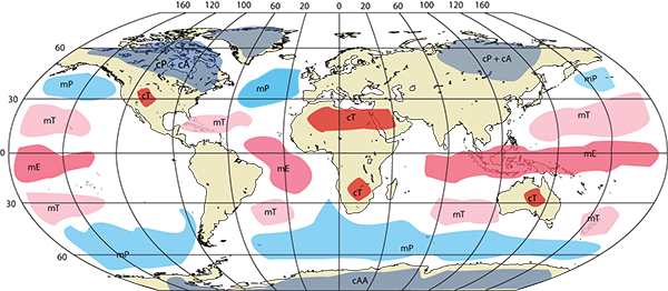
The Role of Clouds and Scattering
Clouds have the ability to scatter and even focus light, which means that sometimes a cloud will remove energy from the solar resource on the ground, and other times clouds will collect and focus light that's even more intense than light on the clearest day in your locale. Yet, we know that clouds are ephemeral and dynamic systems in and of themselves.
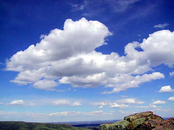
The albedo is the reflective fraction of light from a given surface, a fractional value from 0-1.
Milk, Albedo and Clouds
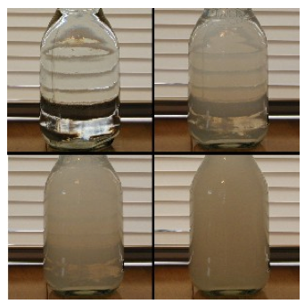
Let's consider a jar of clean water (upper left in the photograph), into which one may add a small amount of milk (upper right). Milk is a "colloidal suspension" of solid particles supported/floating in liquid. As such, the solid particles of fat reflect light, scattering the light in many directions like a cloud would do.
In the lower left and lower right corners, the milk concentration has been steadily increased. We can see through the clear glass of water, suggesting that the transmission of visible light from behind the glass to an observer standing behind the camera is high. For the low concentration mixture of milk and water in the upper right, the small amount of added milk has slightly decreased the transmission of light. We can still see the louvers of the window blinds behind the jar, however.
With more milk added to the mixture in the glass on the lower left, the transmission of light was further reduced, and one's ability to perceive the louvers on the other side of the glass was diminished. Finally, adding more milk to the glass in the lower right cut the transmission of visible light to very low levels, and we can't see through the glass.
What is not being transmitted or absorbed is being reflected. Consider this experiment in the context of albedo. The albedo of clean water in the visible sub-band is much lower than the increasing albedos of all three mixtures of water and milk. Of the three mixtures, the glass with the greatest concentration of milk has the highest albedo.
Recap: we have seen how reflection and albedo is a bit more complicated when light is interacting with millions of surfaces in a suspension, like a cloud. We can also see why a more effective term is backscattered radiation, which is used to describe the collective phenomena. And yet, we can use the backscattered data from clouds to infer useful information about the solar resource at the ground. How do you think we could use that data?
3.10. Climate Regimes
Reading Assignment
- SECS, Chapter 5: Meteorology, the section dealing with Climate Regimes and Space-Time
- Irradiance co-spectrum analysis: Tools for decision support and technological planning, [75] Rayl et al. (2013). Also, available in Canvas Course Reserves.
Time to explore the concept of climate regimes and the influence of meteorological fingerprints in solar resource assessment.
Climate Regimes and Seasonal Fingerprints for Locale
One locale for your client will be divided up into seasons. For us, each season (a block of time) is like an independent region, different from the next season--regions that we will call climate regimes. In the mid-latitudes, we observe four climate regimes, while regions affected by monsoonal swings may have two or three climate regimes.
Recall: there is not one St. Louis, there are four! One for each season, or one statistically different solar resource fingerprint for each synoptic climate regime of St. Louis, Missouri.
Climate regime changes are often noticed by us in terms of the air temperature and humidity, but the sky regimes will change as well, with respect to wind speed, the size of weather cells, and emergent cloud behaviors.
Four different fingerprints symbolizing the different climate regimes for a given locale in winter, spring, summer, and fall. The first fingerprint here is labeled Dec 1 - Feb 28, the second and fourth fingerprints are not labeled. The third fingerprint is labeled June 1st - Aug 31.
I want you to think about the way that seasonal (or synoptic) variations in a locale will generate multiple fingerprints. While each fingerprint is different from another in a given locale (translated: winter solar is not like summer solar), additionally, each set of fingerprints is different from another regional set (translated Mumbai monsoons are not like humid summers in Missouri). Every one of our locales for solar design is going to have "cloudy conditions" at some time, and everyone will have "sunny days" at other times. How can we better understand the variety of intermittencies and trends for our locale and synoptic climate regime (our fingerprint)?
Missouri::Maui::Mumbai
This is just a play on words to emphasize something that you probably can guess: these three locations are not like each other!
- St. Louis, MO [92] is representative of the midlatitude climate regime of the intracontinent. Notably, there are four meteorological fingerprints (seasons).
- Maui (Honolulu, HI [93]) is representative of a Pacific island climate regime, affected by monsoons but without a large landmass.
- Mumbai (Mumbai, Marharashtra, India [94]) is strongly affected by monsoonal swings but is located in the low latitudes of the tropics (two fingerprints).
Self-Check Questions
Please identify the contributions or physical parameters that relate to the solar resource (other than the sun). First look at the questions and write down your answers in your notes. Then scroll over the answers to see how your thoughts match up.
1. What is the role of the sky dome in the solar resource?
Click for answer.
2. What is the role of clouds in the solar resource?
Click for answer.
3. What is the role of aerosols in the solar resource?
Click for answer.
3.11. Discussion Activity
Lesson 3 Discussion in Yellowdig!
We just introduced a totally foreign (yet intuitive) concept of climate regime to our lexicon in solar design. This is a new concept, but an essential one for advanced project development. You can start the discussion by posting what you perceive the meaning of climate regime to be from your personal reading and thought process. You can also comment on any uncertainty you initially found regarding the meaning, the intent, or application of climate regime to a project design, or to long-term project management. Creative interpretations of potential implications are welcome!
Here are some guiding questions:
- What does climate regime have to do with solar resource assessment?
- Is the solar resource a meteorological observable?
- How would you characterize the climate regime at your locale?
- If we wanted to "bin" similar conditions by time, why pick "seasons"? Why not just use monthly blocks?
Tagging
When you create a post in the Yellowdig discussion space, you are required to choose a topic tag. For Lesson 3 discussions, feel free to use any of the following:
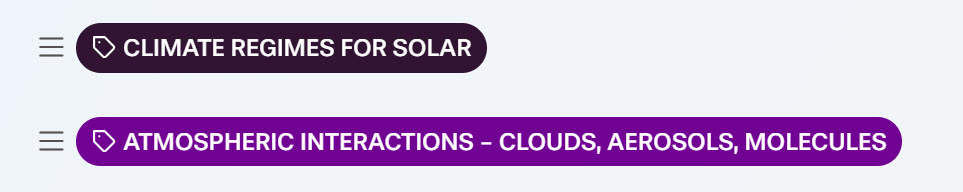
You can tag your post with one or several topics at the same time. All posts and contributions you create are added up to one score at the end of the week.
Importance of interaction
Yellowdig tip: check in the Yellowdig site at least once per day. Commit to making at least one contribution daily – read new posts, ask questions, give your peers reactions and accolades. If reading generates some thoughts, share them, don’t postpone until later. This is a team learning space, so you are also helping others learn by being more active.
Grading
Yellowdig points you earn over the weekly point earning period (from Saturday to next Friday) will count towards 1000 pts. weekly target. But you can go above it (to 1350 pts. max). Yellowdig discussions will account for 15% of the total grade in the course. Check back the Orientation Yellowdig page in Canvas for more details on the points earning rules.
Deadline
There is no hard deadline for participating in these discussions, but I encourage you to create your posts in the middle of the study week (Sunday) to allow others to engage and respond while we are learning specific topics in the lesson. Also, remember that each weekly point earning cycle ends Friday night, so all points accumulated by then will represent your weekly grade, and then you start all over again (it’s like playing a set in tennis..)
3.12. Clear Sky Modeling
Reading Assignment
- SECS, Chapter 5: Meteorology, section dealing with Clear Sky Modeling
- Clear-sky irradiance predictions for solar resource mapping and large-scale applications: Improved validation methodology and detailed performance analysis of 18 broadband radiative models [74] (Gueymard 2012). Also, available in eReserves.
- [Supplemental] Bird and Hulstrom (1981): Simplified Clear Sky Model for Direct and Diffuse Insolation on Horizontal Surfaces, Technical Report No. SERI/TR-642-761, Golden, CO: Solar Energy Research Institute [95]
In the section discussing components of light, we reviewed the effects of the atmosphere on irradiance. Now, we discuss how to model the transparency of a hypothetical sky that is "clear" of the effects of clouds. Clouds are a major contributor to the reduction of terrestrial irradiance; however, particles in the atmosphere also play a significant role. There are physical properties of the sky that we cannot see with our eyes, but which strongly affect the solar resource on a clear day. As we will see in the reading, aerosols and water vapor present in the atmosphere play an important role in scattering light, and they may be present on "clear sky" days when visible clouds are absent.
Daily or monthly irradiance data is required for proper design of any solar energy collection system. However, this data is not always available. This requires the use of well-designed models to estimate irradiance. Hence, the need for clear sky models.
Clear sky models are used to estimate what is called a clearness index. For a location, a clear-sky model must be properly calibrated to provide an accurate measure for the clearness index. We will be looking at two modeling approaches, the Bird Clear Sky Model (which we can download and use as a spreadsheet) and the REST2 model by Gueymard (which can also be downloaded and run as an executable file--we will not do so here).
Bird Clear Sky Model
The Bird Clear Sky Model was developed by Richard Bird and a number of other scientists at what is now the Department of Energy National Renewable Energy Laboratory. The model requires the following input data
- Solar constant (Go, W/m2)
- Zenith angle ()
- Surface pressure (P, (mbar))
- Ground albedo ()
- Precipitable water vapor ([H2O](cm))
- Total ozone ([O3] (cm))
- Turbidity at and/or at 380nm
- Aerosol forward scattering ratio
Many openly available codes incorporate this model. The output is a "clear sky" estimate for the total or global horizontal irradiance (GHI), direct normal irradiance (DNI) and diffuse horizontal irradiance (DHI, or DIF) across wavelengths from 305nm to 4000nm. The model calculates these conditions for a single point in solar time, given the latitude (), longitude () and the Time Zone.
Try this!
Download RReDC: Bird Clear Sky Model [96]
Note: You will be asked to use this tool in this week homework assignment.REST2 Clear Sky Model
The REST2 model has been found to be most accurate, as we shall observe in our reading. We will only need to explore one method (Bird) for this class, but it is important that a resource professional is also aware of the modern application of clear sky modeling. REST2 accepts atmospheric inputs of:
- Air pressure,
- Precipitable water (also as Temp. and relative humidity),
- Reduced ozone and NO2 path lengths,
- Scattering factors for Ångström’s exponents of scattering [97] (wavelengths above and below 700 nm),
- and Aerosol Optical Depth [98] (AOD).
The REST2 model will then output estimations of diffuse horizontal irradiance (DHI), direct normal irradiance (DNI), and global plane of array (POA) irradiance.
3.13. The Role of Clouds
Reading Assignment
- SECS, Chapter 5: Meteorology, section dealing with The Role of Clouds
- [supplemental] Meteorology for Scientists and Engineers, 2nd ed. by Roland B. Stull (Chapter 7). Available under the Modules tab in Canvas in Lesson 3.
Clouds are the big challenge in solar resource assessment. Think about how we just established a "clear sky" model, but most of our skies are filled with clouds that are dynamic and diverse in character. What is it about clouds that makes resource assessment challenging? Take a moment now to familiarize yourself with cloud phenomena and types.
Clouds: the major factor influencing intermittency
Clouds are emergent phenomena within the atmosphere, and strongly perturb the behavior of the solar resource in a given locale. When we do not have a clear sky day in our locale (typical in many locations on Earth), the effects of clouds will strongly draw down the beam component of our solar resource and increase the net fraction of diffuse sky irradiance.
Clouds can develop in environments that are termed active and passive, as well as from updrafts near the Earth’s surface. As we have seen in the reading, clouds have the ability to either scatter and reduce incident light, or to act as a lens at the perimeter, focusing light well above clear sky or even AM0 irradiance conditions.
From the perspective of an observer standing on the Earth's surface, clouds can be classified by their physical appearance. Accordingly, there are essentially three basic cloud types:
- Cirrus, which is synonymous with a "streak cloud" (detached filaments of clouds that literally streak across the blue sky),
- Stratus, which, derived from Latin, translates to a "layered cloud," and
- Cumulus, which means "heap cloud."
Let's review some basic types of clouds. Please do comparative reading between the figure below (with images) and your list of cumuliform, stratocumulus, and stratiform clouds in Ch. 5 of SECS.
-
Cirrus (Ci): Clouds characterized by thin, wispy strands, forming in either patches or streaks. No uniformity (either in clumps or layers) in such clouds are usually observed. Cloud edges are not distinct and there is generally no shading of cloud elements.
-
Cirrocumulus (Cc): High cloud composed of very small but distinct cloud elements. Elements may in turn be arranged in patches or waves. Individual cloud elements are uniform in appearance and show no shading (and may appear at times to be translucent).
-
Cirrostratus (Cs): High, thin, generally uniform sheets of clouds formed by ice crystals. Sun/moon is brilliantly observed through the clouds which often produced optical phenomenon such as halos.
-
Altocumulus (Ac): Mid-level cloud consisting of globular masses or rolls in layers, lines, or patches. Individual cloud elements are usually white or gray with a minimal amount shading. Cloud edges are distinct due to their composition of water droplets.
-
Altostratus (As): Mid-level cloud of uniform density displaying no distinct features over the entire layer. Sun can usually be observed, but is often quite dim and does not display any optical phenomenon.
-
Cumulus (Cu): Low-level convective cloud with flat bases and distinct outlines. Fair weather cumulus exhibit only slight vertical growth, with the cloud tops designating the limit of the rising air.
-
Cumulus-congestus (TCu): Vertically developed clouds that are usually twice as tall as they are wide. Clouds exhibit hard, distinct boundaries along their top edges, lacking a fibrous anvil.
-
Cumulonimbus (Cb): A towering, vertically developed cloud occurring individually, in clusters, or lines. Clouds display a characteristic anvil at it's top and are most often accompanied by rain, gusty winds, and (occasionally) hail.
-
Stratocumulus (Sc): A layer of cloud consisting of large dark, rounded masses, usually in groups, lines or waves. Cloud bases can be quite low, but individual cloud elements are fairly shallow in vertical development. Little, if no, precipitation is observed from such clouds.
-
Stratus (St): Low, gray, uniform clouds usually covering the entire sky and persisting for an appreciable period of time. Clouds may produce some intermittent drizzle or snow flurries but are not characterized by persistent or significant precipitation.
-
Nimbostratus (Ns): Low, gray, uniform clouds usually covering the entire sky and persisting for an appreciable period of time. Characterized by constant rain or snow of light to moderate intensity.
Clouds are listed here with images that pop up when you click on the red dots. We see variants of cumuliform clouds, stratocumulus clouds, and stratiform clouds, as noted in our reading.
There are four general classifications of clouds: high, middle, and low clouds as well as clouds of vertical development. The table below summarizes each of these classifications while giving you a sense for the typical altitudes at which their cloud ceilings (the height of their bases) are observed, and the basic chemistry of the clouds (ice and water interact with light in different ways).
| Type of Cloud | Definition | Image |
|---|---|---|
| High Clouds | Observed over the middle latitudes. Typically reside at altitudes near and above 20,000 feet. At such rarefied altitudes, high clouds are composed of ice crystals. | 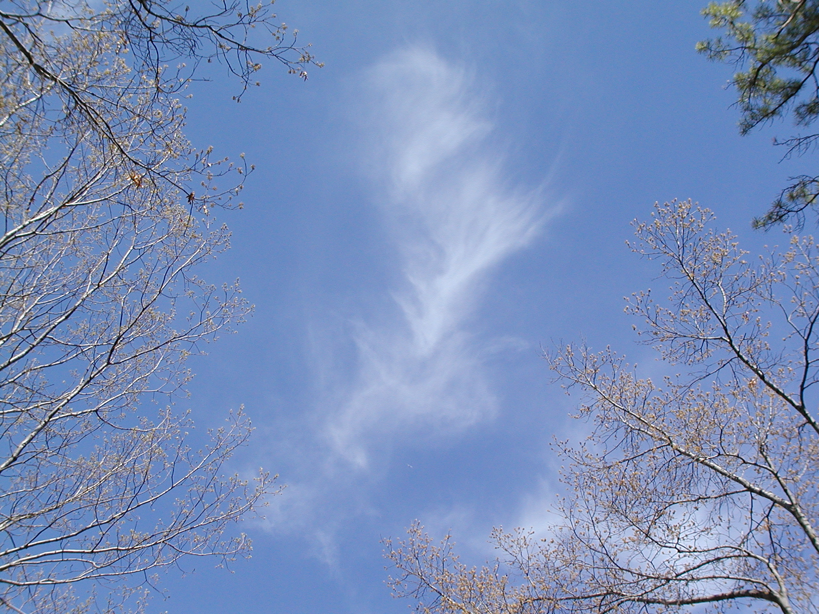 [99] [99] |
| Middle Clouds | Reside at an average altitude of ~10,000 feet over the middle altitudes. Keep in mind that this is an average altitude, so middle clouds can form a couple of thousand feet above or below the 10,000 foot marker. Middle clouds are composed of water droplets and/or ice crystals. | 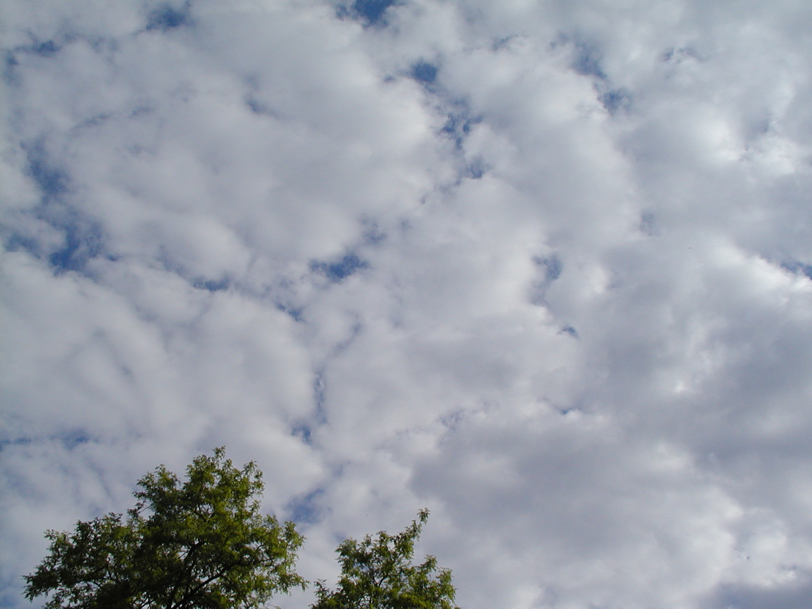 [100] [100] |
| Low Clouds | Can form anywhere from the ground to an altitude of approximately 6000 feet. For the record, fog is simply a low cloud in contact with the earth's surface. |  [101] [101] |
| Clouds of vertical development | Cannot be classified as high, middle, or low because they typically occupy more than one of the above three altitude markers. For example, the base of a tall cumulonimbus cloud often forms below 6000 feet and then builds upward to an altitude far above 20,000 feet. | 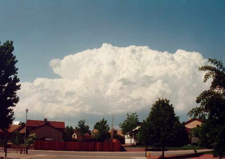 [102] [102] |
Recapping: You should begin to think about how clouds can both block the beam component of light from the Sun (making the skydome more diffuse in nature), and can refract and scatter light like a lens, increasing the irradiance on a locale far higher than predicted from a clear sky model.
- Blocking beam irradiance
- Enhancing beam irradiance through "lensing" over a local site (effects can last several minutes locally)
Researchers are now trying to predict cloud behavior with respect to GHI and DNI variation in a given locale. We are still a few years off, but soon we may see solar forecasts that include cloud interference for solar resource assessment.
Acknowledgment: Content of this page comes from Meteo 101: Understanding Weather Forecasting; author: Lee Grenci and David Babb.
3.14. Taylor's Hypothesis
Reading Review
SECS, Chapter 5: Meteorology, "Robot Monkey Does Space-Time" section
When we look at clouds, think of how they float by us without really changing in form all that much. Kind of like train cars passing by on the railroad, only much slower. We can use this to connect space and time (or frequency) in a useful way for solar resource assessment.Clouds (and weather fronts) occur on multiple scales of space and time. These scales contribute to the concept of solar fingerprints or climate regimes. In our reading, we learn about Sir Geoffrey I. Taylor and his work on turbulence theory. Clouds lead to intermittent solar conditions (POA and DNI irradiance) that, in turn, affect our solar energy conversion technologies, such as PV and building systems.
The intermittent variation of clouds as they affect the solar resource is crucial when solar is deployed as a large-scale farm, or as a large community of decentralized PV arrays on buildings. Variable peaks and valleys of electrical power can be detrimental (costly) to utilities if there are no other ways to store or shave variation on the grid. Now, storage solutions are emerging slowly in research, but right now we need to address the intermittency problem by better understanding the drivers and the basic science underneath those drivers.
Taylor's Hypothesis:
A series of changes in time at a fixed place is due to the passage of an unchanging spatial pattern over that locale. That is, when observing a cloud or thunderstorm passing overhead, the clouds of the thunderstorm floating by are effectively "unchanging spatial patterns" (big blocks of cloud). Put another way, the lateral change in the cloud conditions across regions of the meteorological event (e.g., cloud-sky-cloud-sky-cloud) can be directly connected locally with a variation in irradiance measurement over time (e.g., a periodic measure of dark-bright-dark-bright-dark).
Taylor’s hypothesis states that events that change in time for a fixed place are due to the flow or passage of unchanging spatial patterns over a locale. This is like observing a thunderstorm passing by directly overhead and making the connection to the rate of the clouds advecting with the thunderstorm. Taylor's hypothesis from the 1930s allows us to flip from the Eulerian frame of reference (time sequences) to the Lagrangian frame of reference (spatial changes).
The Eulerian frame of reference: When an observer is stuck in one place, only watching the changing phenomena as it passes by.
The Langrangian frame of reference: When the observer moves with the meteorological phenomena instead of remaining fixed. Imagine a flying carpet floating along with a cumulus cloud moving from one county to the next.
Hence, all scales of time (or frequency) are also spatial scales! Taylor's Hypothesis holds so long as the advective wind speed is much greater than the timescale of the evolving meteorological event being investigated, as is often the case. When you have a lazy cloud day, where the clouds are changing form faster than they move, the time-space connection doesn't hold anymore.
Connecting Scales of Space with Time
By using spatio-temporal scales of cloud features established by Ted Fujita, we can estimate an average translation (advection) speed of 17 m/s for meteorological phenomena. We can then convert the spatial scales of variability into a relevant timescale. Spatial scales associated with power transmission congestion are distances of 25-1000 km. These distances are relevant for meteorological phenomena within time scales on the order of 25 seconds to 16 hours.
Cumulus 2-5 km, which means 10-100 minutes.
Cumulonimbus (including anvil) 10-200 km, which means 1-5 hours.
Cumulonimbus cluster (including merged anvils) 50-1000 km, which means 3-36 hours.
Synoptic (including cyclone waves, short and long Rossby waves) 1000-40000 km, which means 2-15+ days.
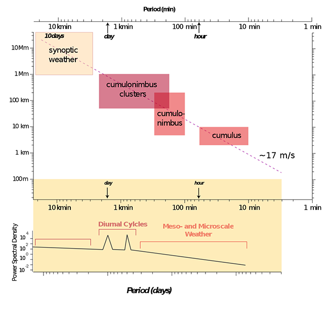
If we plot all of these phenomena and draw a line down the middle, we have a really rough estimate of the average advection rate of meteorological phenomena on Earth. Here, we have represented that rate in three different unit scales:
- 17 m/s [easy to remember this one, 17 is a prime number] or
- 1 km/min
- 61 km/hour (or 1470 km/day)
- 38 miles/hour (or 913 miles/day)
As such, we can connect Synoptic, Mesoscale, and Microscale meteorological phenomena between spatial and temporal scales!
General Scales of Meteorology in Space and Time:
Synoptic Weather: This is weather on the scale of 1000+ km in distance, and (given advection of ~17 m/s) seasonal timescales of 2-15+ days.
Mesoscale Weather: This is weather phenomena, including solar condition, on the scale of 100-1000 km distances, and time scales less than one day (hours).
Microscale Weather: This is variable weather phenomena on the scale of 10-100 km distances, and time scales of minutes to seconds.
Taylor’s Hypothesis “works” when the air in the sky moves significantly faster (advection: wind speeds) than the evolution time of a cloud or a thunderstorm of clouds. So, this approximation breaks down for those days when the cumulus clouds just "hang" in the sky all day.
Self-Check
3.15. Learning Activity: Clear Sky Model
Clear Sky Model and Measured Irradiance Data
The following readings will be helpful for completing this lesson activity.
Readings:
- SECS, Chapter 6 - Sun-Earth Geometry
- Supplemental: SECS, Chapter 8 - Measure and Estimation of the Solar Resource
Especially:
- pp. 159-161 of Moments, Hours, and Days [Ch 6] (see a breakdown of Equation 6.19 for I0)
- p. 217: Empirical Correlations for Components [Ch 8] (see Fig. 8.5)
- p. 221: Clearness Indices and Climate Regimes [Ch 8]
- p. 226: Diffuse Fraction [Ch 8] (Eq. 8.24 is related to hourly components)
Tasks
The goal of this activity is to use the BIRD Clear Sky Model to predict the solar irradiance at a specific time at a specific locale and further compare those predictions to actual irradiance measurements.
So there are two main tasks in this activity:
- Download and learn how to use the Bird Clear Sky Model (predicted irradiance)
- Download and plot the SURFRAD Measured Data (measured irradiance)
These two tasks will be performed for a specific date - July 31, 2007 (in this assignment) for the specific locale - SURFRAD Meteorological Station at Rock Springs, located just outside State College, PA.
In the end, you will need to assess how the modeled (predicted) and measured data fit and provide some discussion on it.
Part 1. Bird Clear Sky Model - Instructions
The Bird model is an old but advanced clear sky model used by solar professionals to estimate clear sky conditions at a locale. The clear sky model for a horizontal surface is the basis for almost all modern comparisons of "ideal skies" to actual skies (with clouds and dynamic light interference effects). You will see what the global, beam horizontal, and diffuse components of solar light should look like when you set the meteorological parameters affecting the sky clearness. The model could also provide DNI (Direct Normal Irradiance), which would show irradiation values higher than the global horizontal values for the mornings and evenings.
- Go to http://rredc.nrel.gov/solar/models/clearsky/ [96] to download the Bird Clear Sky Model. It is a free download, and the tool comes in the form of an Excel spreadsheet. I suggest that you rename the original file for any case study you perform further.
- Study the instructions on the spreadsheet to learn how to use the tool and make a note of the input and output parameters.
- Modify the inputs for the State College, PA, locale. The following parameters can be obtained from the SURFRAD site (see part 2):
- Latitude 40.72
- Longitude -77.93
- Time zone UTC -5
- Pressure (mbar) - average for the day
- Aerosol optical depth (AOD)
Note: access the AOD data through this graphical page [103]. Take the daily average as input for the Bird model. In this case, 415nm AOD can be used as a proxy for 380nm AOD input and 500nm AOD data can be used as is.
- You can leave other inputs at their default values
- Expand the spreadsheet (as explained in the instructions) to generate output for the entire year, then extract the data for July 31st (day # 212) and copy values to a separate file.
- Plot global horizontal irradiance (GHI), direct horizontal irradiance (DHI), and diffuse horizontal component (DIF) versus time for the day
The model plot will look similar to the one below. This is what you need to produce.
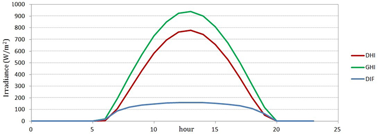
Part 2. SURFRAD data - Instructions
The SURFRAD site at Penn State collects real-time data for solar irradiance (using local pyranometers) and a number of other atmospheric parameters at 3-minute time intervals. These data are accessible through the Earth System Research Laboratory website [104]. This site provides you with access to data collected at the Penn State location. For each year, you can open the parent directory with .dat files, which are named by the day number. So if you are looking for July 31st, for example, that will be day #212, so check the file psu07212.dat.
Your goal will be to make sense of these data, extract your irradiance values and plot them versus time of the day.
Here are the data labels in order that correspond to the numbers in the .dat file (omit 0-value columns):
Year, jday, month, day, hour, min, dt (decimal time), zen (degrees), dw_solar (W/m^2), uw_solar (W/m^2), direct_n (W/m^2), diffuse (W/m^2), dw_ir (W/m^2), dw_casetemp (K), dw_dometemp (K), uw_ir (W/m^2), uw_casetemp (K), uw_dometemp (K), uvb (mW/m^2), par (W/m^2), netsolar (W/m^2), netir (W/m^2), totalnet (W/m^2), temp (degC), rh (%), windspd (m/s), "winddir (degrees, clockwise from north)", pressure (mb)
From this list, you will specifically need:
dt (decimal time) - your time coordinate for data plotting (Column G in MS Excel)
dw_solar - Downwelling global solar (W/m^2) = corresponding to Global Hz (GHI) in BIRD model (Column I in MS Excel)
netsolar - Net solar (W/m^2) = corresponding to Direct Hz (DHI) in BIRD model (Column AG in MS Excel)
diffuse - Real downwelling diffuse solar (W/m^2) = corresponding to Dif Hz (DIF) in BIRD model (Column O in MS Excel)
Also, 'pressure (mb)' - the last value in each array of data - daily average should be used for your Bird model input (Column AU in MS Excel).
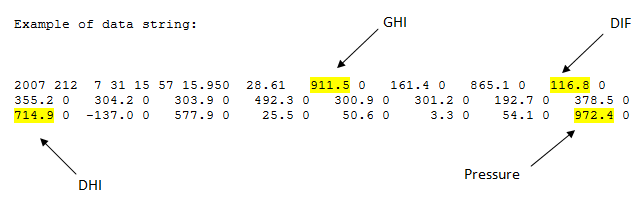
2007 212 7 31 15 57 15.950 28.61 911.5 0 161.4 0 865.1 0 116.8 0
355.2 0 304.2. 0 303.9. 0 492.3 0 300.9 0 301.2 0 192.7 0 378.5 0
714.9 0 -137.0 0 577.9 0. 25.5 0 50.6 0 3.3 0 54.1 0 972.4 0
911.5 = GHI
116.8 = DIF
714.9 = DHI
972.4 = Pressure.
To treat the data, you can either convert the .dat file to a spreadsheet (see video in Canvas Module 3 how to!) or, if you have programming skills, you can create a script to plot the irradiance data versus time.
Important Note: you may notice that the "0" decimal time in the .dat file does not correspond to the actual local midnight, but rather corresponds to Greenwich 0:00, so you may need to synchronize decimal time with the Bird model to make the calculated and measured curves match.
Comparison and discussion of the results
- Plot the Bird model data and SURFRAD measured data for GHI, DHI, and DIF types of irradiance on the same diagram. You should get a pretty close match. You may notice by visually comparing the curves, that even on a clear day, the real sky shows dynamic variations in irradiance in the diffuse component.
- Provide a discussion of the results and comment on the possible discrepancies.
Submitting Your Work
Prepare a written report including the following:
- Table of input parameters for the Bird model (left side of the Bird spreadsheet)
- Diagram with irradiance data comparison (Bird model vs. SURFRAD data points)
- Discussion of results.
Save your report as .docx or PDF and submit to the Lesson 3 Activity - Clear Sky Model dropbox in Canvas.
Grading Criteria
Please see the grading rubric in Canvas
Deadline
See the Calendar tab in Canvas for specific due dates.
3.16. Summary and Final Tasks
Summary
In this lesson, we have learned about the diverse ways in which the atmosphere can interact with shortwave light to affect the solar resource received at the ground by our Solar Energy Conversion Systems. We have observed that the sky has a distinct character derived from air mass source regions, and that the weather has seasonal "fingerprints" that distinguish a single site as multiple unique climate regimes. We further found that a "clear sky" is a fairly complex system of its own, and modeling the clear sky is not trivial. When we finally add clouds to the skies, we see where the real source of solar intermittency stems from. By connecting space and time from Taylor's Hypothesis, we find that we hold additional information on the scales of intermittency to expect in a given locale and for each seasonal climate regime in that same locale.
Reminder - Complete all of the Lesson 3 tasks!
You have reached the end of Lesson 3! Double-check the to-do list on the Lesson 3 Learning Outcomes page to make sure you have completed all of the activities listed there before you begin Lesson 4.
Lesson 4 - Measurement and Estimations of the Solar Resource
4.0 Overview
Overview
This is the last big push to bring everyone in the class up to speed on solar resource topics, so stick with it, folks! We will be learning a lot more about measuring light directly in the field relative to estimated light calculations based on empirical (data-driven) correlations.
Why do our eyes create so much bias in determining solar decision making? Is there something better than vision to compare the solar resource? Is the human eye really designed to be a solar detector of intensity? It's time to come eye to eye with our embedded ethics of measurement in society. More on that soon!
We use the concept of components to break the sky dome and the ground into digestible chunks of surfaces with common emission/absorption/ scattering characteristics (e.g., direct, Gb, diffuse, Gd, circumsolar diffuse, ground reflected diffuse, Gg). Components of global irradiance relate to the sources of light within the sky dome. A component is a term for the groups of physical orientations and scattering of light (e.g., diffuse component, beam component). The characteristic measures are assessed within temporal blocks as statistical summations of irradiation on a horizontal surface (e.g. G / I / H / H-bar / annual) and the degree of light scattering found on a horizontal surface via the clearness indices (e.g., kT, KT, K-barT ).
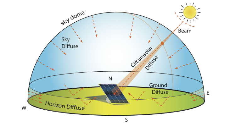
We shall see that when it is challenging or costly to measure multiple components of light (scattered and unscattered), we have old and somewhat dated tools to attempt broad estimations on the contributions of each component to the total irradiation incident on the aperture of interest. You will see how we often rely on historical observations and empirical correlations by solar scientists and engineers for hourly, daily, and monthly average day data. The main tools used for these older equations are both measured hourly Global Horizontal Irradiation (GHI, or I) gathered from a horizontally mounted pyranometer, and daily extraterrestrial irradiance (Air Mass Zero = AM0, or Top Of Atmosphere = TOA, or just I0), which you learned about in the last chapter. We shall also find that one can infer more than just the components of light from the ratios of measured irradiation to AM0 calculated irradiation--however, there can be significant errors included in the process. We can also describe the fractions of days in a given month where lighting conditions will be clear or overcast/cloudy.
You will also see reference to the Typical Meteorological Year. Keep an eye out for that...it will be a major part of SAM simulation software.
Math warning!
You will observe several equations that are long and complicated. They are empirical relations that will be used to estimate the solar resource on non-horizontal surfaces. As with prior lessons, these equations are at the core of software like SAM, and a student completing this course should be very familiar with their application. Stick with it!
4.1 Learning Outcomes
By the end of this lesson, you should be able to:
- explain why the human eye is a poor solar detector and creates bias in decision making;
- describe the equipment used to measure irradiance and irradiation in the field and from space;
- contrast collecting data for horizontal irradiance and DNI with (Plane of Array) POA measurements;
- describe the meaning of a component of light, and list the components for anisotropic skies on a tilted surface;
- explain scenarios where direct POA (Plane of Array) measurement is not available and one must use empirical correlations (via clearness indices) to estimate irradiation on a horizontal surface;
- understand and be able to apply typical meteorologic year (tmy) data to energy system simulations.
What is due for Lesson 4?
This lesson will take us one week to complete. Please refer to the Course Syllabus for specific time frames and due dates. Specific directions for the assignment below can be found within this lesson.
| Required Reading: |
J.R. Brownson, Solar Energy Conversion Systems (SECS), Chapter 8 - Measure and Estimation of the Solar Resource. D. T. Reindl, W. A. Beckman, J. A. Duffie (1990) Diffuse Fraction Correlations [105]. Solar Energy. 45(1) 1-7. |
|---|---|
| Optional Reading (not required): | Liu and Jordan (1960) The Interrelationship and Characteristic Distribution of Direct, Diffuse, and Total Solar Radiation [109]. Solar Energy J. 4(3), 1–19. S. Wilcox and W. Marion (2008) Users Manual for TMY3 Data Sets [110]. NREL/TP-581-43156 S. Wilcox (2012) National solar radiation database 1991- 2010 update: User’s manual [111]. NREL/TP- 5500-54824 Perez, Ineichen, and Seals (1990) Modeling Daylight Availability and Irradiance Components from Direct and Global Irradiance [112]. Solar Energy J. 44(5), 271-289. |
| To Do |
Learning Activity: Clearness Index calculation Discussion: Typical Meteorological Year Quiz Assignment: Components of Light (see Canvas) Engage in all Try-This and Self-check activities (not graded). |
| Topic(s) | Irradiance/irradiation measurement (ground vs. satellite) Horizontal Surfaces: Day/Month/Hourly Clearness Indices Typical Metrological Year (TMY) Tilted surfaces: Isotropic/Anisotropic sky models and POA Direct Normal Irradiance |
Questions?
If you have any questions, please post them to the Lesson 4 General Questions and Comments Discussion Forum in Canvas. I will check the forum regularly to respond. While you are in a discussion, feel free to post your own responses if you, too, are able to help out a classmate.
4.2 Vision is a significant bias to assessing the Solar Resource
Reading Assignment
- J.R. Brownson, Solar Energy Conversion Systems (SECS), Chapter 8: Measure & Estimation of the Solar Resource (section on Human Vision).
As modern society, we each seem to lack a cultural awareness for measures of light per radiometry is our biological link to vision. Along with your reading, think about why your vision has quite different criteria for performance than a solar hot water panel, or a PV module. I would like you to shift your metrics from clarity and information, linked with photometry, to that of irradiance on a given surface. We present this page to "illuminate" our collective bias that vision brings in to our solar resource estimations.
Read the following description of your eyes, and think about the type of equipment that we will need to assess the solar resource for economic decision-making. There are numerous physical challenges incorporated into vision that strongly bias perception of a solar resource. But solar resource assessment is about metrics (physical measurements), not perception.
Consider: I have personally heard people tell me that solar technology is not viable in Pennsylvania, North Dakota, and Minnesota. The news media have erroneously stated solar is too diffuse for all of the United States (old Fox News report: because Germany was supposed to be brighter?). Additionally, my colleagues have been told stories that solar is not viable in places such as Santa Barbara and San Francisco, as well.
None of these armchair philosophy assessments is correct. First, speculation on the solar resource using visual cues is not appropriate; our eyes do not actually measure the solar resource in a meaningful way for SECSs. Second, speculative resource arguments (even measured data) must ultimately be tied to economic arguments. Here, we lack the financial argument (the economics) associated with the avoided cost of fuels from incorporating solar energy technologies in a given locale for a client of interest. We will cover the financial and economic discussion in the next lessons to come, but let's go back to vision for a moment.
Sight Perception is a funny thing
Sight perception works to our advantage as individuals when we wish to minimize risk, such as avoiding that lion prowling through the forest in the evening. It also adapts with weak or intense signals, trying to feed the brain a useful stream of information. As such, sight also has limitations, in that our sensory systems are combined with a cognitive system to extrapolate small signals into big information or really intense signals into reasonable information. The goal of sight is information about the world around us, not the amount of light delivering that information to us.
How does the eye work?
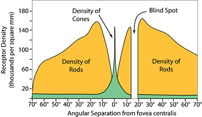
The eye has two main conversion molecules: rods and cones, located in the retina. The two systems have adapted for dim lighting (rods) and full daylight. Rods absorb only certain wavelengths of light that are longer and lower energy, while the system of cones (actually multiple kinds of cones) absorbs the wavelengths of light that we interpret as color. In both systems of absorption, the maximum range of wavelengths is limited and does not include the ultraviolet and infrared regions that comprise about 50 percent of the shortwave band of solar irradiance. So, our eyes do not detect a large range of solar wavelengths, and the response factor of those receptors is not linear either. This is a detraction to using the eye as a quantitative solar detector.
Notice in the figure that the rods and cones are distributed across the back of the eye, but the two systems are not distributed in the same fashion. Rods are distributed broadly across the retina, with the exception of the fovea centralis. In complement, cones are distributed tightly within the fovea centralis. The two distributions are linked to the lens system of the eye.
- Cones: found mainly at the focal point of our lenses, the fovea centralis
- Rods: found distributed everywhere except at the fovea centralis
The lens system in the eye conveniently allows us to think about concentrating solar systems ahead of schedule (CSP, concentrating solar power for thermal steam production; and CPV, concentrating photovoltaics for electricity production).
Any lens will focus light onto a focal point (the fovea centralis here), but can only collect light from the direction that the lens is pointing. Meaning, a contracting system has to track the bright light sources for better performance.
The implications of this property of concentrating optics is that cones will only detect light in the direction that the eyes are pointing. So, our color detection system is relatively poor at sensing diffuse or scattered light from areas of the sky or ground at which the eye is not pointing. Mark one more detraction for the eye as a solar detector.
Going back to the rods...they are distributed everywhere except the focal point, and so will detect diffuse light entering the eye from all angles. Recall that rods are not color sensitive; they just detect long wavelength photons, such as those at night or during the twilight. If you want to see more at night while riding a bike or running, you are encouraged to defocus your vision to allow peripheral light to be detected. The optical implications are that your rods are not part of a concentrating system and will detect diffuse light better at the expense of color discrimination, but only at low levels of light. Mark yet another detraction for the eye as a quantitative solar detector.
And now, your additional macroscopic feedback system to control light acceptance, the iris. As the object of your eye is to provide your brain with the best information, not power, the iris is a feedback system meant to open wide when the light is dim, and squeeze up small when the light is intense. No matter what your rods and cones are doing, your iris is constantly adapting to maximize the signal of visual information to the brain. In a power detection system, we do not want an adaptive iris system, because it again detracts from our goal of linear detection of irradiance changes across the day.
We can also add the eyelids and eyebrows to your optical system, as they block or shade much of the bright light to your eyes. We can add behavior to our eye system, in that very few people actually look up to sense the light in the sky, and tend to look to the horizon instead, meaning our lenses are not trained vertically upward, but more along a horizontal plane (we mount solar detectors flat, to point up to receive the entire sky dome of light). All in all, we can come to the conclusion that the eye is not the ideal constant solar detector to inform us quantitatively of the amount and changes in irradiance during the day.
Power vs. Information
When a device takes one form of energy as an input and transforms it into different new forms of energy as outputs, the process is called energy conversion. The source of that input energy is called a resource. Now, if we were to draw upon the resource of the Sun from the point of a dude on Earth's surface, the energy form is electromagnetic radiation. We will call this light, bearing in mind that light from the Sun can be visible or invisible (ultraviolet and infrared) to the eye.
If one wished to transform the light into an electronic, or electrochemical signal, the resulting device (an energy conversion system) could be tailored to provide lots of power (more energy, less information) or to provide lots of information (less energy, more information). Let's use two examples: a photovoltaic cell (solar-electronic transducer), and the human eye (solar-electrochemical transducer).
- The photovoltaic cell is designed to respond in a linear fashion to the intensity of solar irradiance, thus delivering the maximum amount of power, but not functioning well at all in the night or during twilight. The device will provide changing levels of voltage and current (voltage times current is power) in a direct linear response to the intensity of irradiance.
- The human eye is designed with an iris, rods and cones, and lenses to respond in an adaptive, logarithmic fashion to the intensity of solar irradiance. The eye will detect the tiniest of solar signals on a starry night, and will adapt to the brightest of desert suns during the day, while always providing very similar levels of electrochemical voltage and current to the brain, but with a high degree of information content that can separate the light reflecting from a "lion" vs. a "tiger" vs. a "bear." A device that can sense a signal over many orders of magnitude is a logarithmic detector.
Summary
The eye is designed to provide you with the information sufficient to avoid bumping into bad things in extreme lighting conditions. This is called information, but it is not the useful information for assessing the solar resource quantitatively. A linear detector like a photovoltaic device is required to accurately measure the power of the solar irradiance.
Self-Check
4.3 Measurement devices: Technology of irradiance transducers
Reading Assignment
- J.R. Brownson, Solar Energy Conversion Systems (SECS), Chapter 8: Measure & Estimation of the Solar Resource (Focus on instrumentation.)
- Sengupta et al. (2015) Best Practices Handbook for the Collection and Use of Solar Resource Data for Solar Energy Applications [107]. NREL/TP-5D00-63112: p. 19-62: Chapter 3. Measuring Solar Radiation
Why Measure?
Measurement is an important aspect of all scientific endeavors. It is especially important in the proper and efficient design of solar energy collection systems. Proper solar assessment involves metrological and climate data, and correct measurement of global (beam and diffuse) radiation is essential to any solar design effort. Without adequate and precise measurement of the solar resources, system designers and engineers would essentially be "flying blind." In this section, we will discuss the equipment used to perform the required measurements.
Video: Measuring sunlight - Edited version for World Meteorological Day 2019 (4:36)
The Sun. This constant companion delivers the energy that powers life on Earth. But for over four and a half billion years of Earth history the amount of energy the earth has received from the Sun has varied, with major consequences for the climate and for living things. Even the relatively stable climate humanity has enjoyed since the end of the last Ice Age is regularly affected by small changes in the amount of solar radiation reaching the Earth's surface.
These small variations are caused by long-term cycles affecting the Earth's orbit around the sun, changes in cloud cover, and other fluctuations here on Earth. They can have major impacts on our lives. The 1991 volcanic eruption of Mount Pinatubo, for example, spewed huge clouds of sulfur aerosols into the air. This reduced the sun's irradiance by up to 5 percent for around ten months, which cooled the Earth by some point 5 degrees Celsius for several years. This is why measuring the sunlight hitting the earth is so important. It is critical to our understanding of the weather and climate system.
Scientists need radiation measurements in order to study climate variability and change and to forecast the weather. Radiation measurements are also essential for decision-makers in the solar energy industry. To calculate how much electricity a proposed solar energy installation will produce, they need to know how much sunlight will be available on sunny days, and cloudy days, or on short winter days versus long summer days. Measuring sunlight, however, is not as easy as it may sound. We need long-term measurements that are comparable from place to place, from time to time and from instrument to instrument. This requires a special effort to finally calibrate thousands of ground-based instruments all around the world.
The P.M.O.D. Institute in Davos, Switzerland has been studying how to measure sunlight for over 100 years. Since 1959 it has organized a meeting every five years bringing together scientists from around the world to simultaneously calibrate their instruments. In 1971 the World Meteorological Organization invited the P.M.O.D. to serve as the world radiation Center. The center maintains the primary standard for measuring the Sun's irradiance, the so-called world Radiometric Reference. This ensures that these highly sensitive instruments, known as pyrheliometer, are accurate and their data are comparable. Accuracy is particularly important for the solar energy industry, which needs to know the absolute amount of sunlight that is available, while comparability is critical for climate science, which tracks trends and changes over time. Wolfgang Finserele is responsible for solar radiometry at the WMO World Radiation Center. He maintains the “World Standard Group” comprising the six measuring instruments against which instruments around the world are compared.
Our role is to make sure that everybody uses the same accurate scale for measuring solar irradiance. To make those measurements comparable to each other and two measurements that I can take in the past and we'll be taking in the future. Without international collaboration on carrying out this rigorous behind-the-scenes work, we would have a much weaker understanding of the climate system. Without the IPC, countries can't compare their radiation data. We would not be able to look at effective climate records throughout the globe, so this is a very vital important part of the role of the WMO. The World Radiation Center will organize the next global intercomparison meeting in 2020 and will continue its work on assuring the quality of solar radiation measurements far into the future.
Pyranometers and Pyrheliometers
The Pyranometer: Global Irradiation Measurements
Pyranometers act as solar energy transducers, in that they collect irradiance signals and transform them into electrical information signals. That information is passed on to a data logger and computer, and then we either present the data in short bursts (1 second) or integrate and average the data over longer periods of 1 minute to 1 hour.
Research grade pyranometers use a film of opaque material to collect thermal energy. The thermal energy diffuses into a thermal transducer called a thermopile (a stack of thermal devices) that produces a small current proportional to the temperature. We should note that metals (in general) are very good reflectors, making them also very poor absorbers. So, how do we get a material that functions on thermal gradients to make use of the radiation from the sun?
The key is in the absorber material: Parson's black is a paint with very low reflectance across shortwave and longwave bands of light (~300-50,000 nm; making it an effective blackbody). However, if covered by glass (a selective surface), the "window" of light acceptance from the Sun is about 300-2800 nm. This system assembly forms a shortwave (band) global (component) pyranometer. Now imagine, if we develop a thermopile with a thin coating of a black absorber, but replace the glass with a material that is transparent in the longwave band (many organopolymers/plastics), we will have created a longwave (band) global (component) pyranometer.
On the other hand, inexpensive pyranometers can use photodiodes. Photodiodes are photovoltaics (just small). They are semiconductor films that directly convert shortwave band radiation into electrical signals (no thermal conversion step necessary). While the cutoff for a silicon photodiode is <1100nm, the integrated power response is fairly comparable to that of a Parson's black-coated thermopile detector. However, they do not perform as well (relative to thermopile detectors) near sunrise and sunset due to a cosine response error.
Cosine Response Error
Remember the cosine projection effect that we discussed in Lesson 2? It matters here for solar measurement. In the morning and evening, at low solar altitude angles (), some of the radiation incident on the detector is reflected, which produces a reading less than it should be. Some correction can be made for this using a black cylinder casing and a small white plastic disk cover (with a low reflectance at low angles to minimize the cosine error).
Review of a pyranometer in operation:
For standard research, technicians mount pyranometers in a horizontal orientation. Pyranometers produce a voltage in response to incident solar radiation. Provided that a pyranometer uses a thermopile (thermoelectric detector), the device acts as an "integrator" of all components and bands of light. In the case of a glass enclosure, even a thermopile detector will operate only in the shortwave band. Pyranometers based on photodiodes are used only for shortwave global radiation measurements. The following two images are explained in detail at the University of Oregon's Solar Radiation Monitoring Laboratory [70] (maintained by Dr. Frank Vignola). The left image is a LI-COR pyranometer [115], which uses a silicon photodiode to measure irradiance (a little PV cell). The right image, which looks like a flying saucer from the 1950s, is an Eppley Precision Spectral Pyranometer (PSP) [116]. The Eppley is a First Class Radiometer, and uses a thermopile to measure irradiance. The white ring is to reflect stray light away, such that the system does not heat up and so that the influence of the ground reflectance (the albedo) is minimal.
Standard pyranometers are designed to be mounted horizontally in shadow-free areas, with the normal vector relative to the surface of the collector (which is horizontal) pointing vertically. Measurements of downwelling shortwave band irradiance from a horizontal pyranometer collect Global Horizontal Irradiance, or GHI. However, through a simple modification, a pyranometer may also be used to measure diffuse irradiance. By using an occulting disk or band, beam radiation can be blocked from the sensor surface of the pyranometer, leaving only diffuse radiation to be measured.
The Pyrheliometer: Beam Component Measurements
If we wished to measure only the direct component of downwelling irradiation, we would use a pyrheliometer. The device is a combination of a long tube with a thermopile at the base of the tube and a two-axis tracking system to always point the aperture of the device directly normal to the surface of the Sun. A measure of irradiance from a pyrheliometer is therefore called Direct Normal Irradiance (DNI) (Gb,n) data. An Eppley Normal Incidence Pyrheliometer [117] is displayed below on the left, while an Eppley Solar Tracker [118] is displayed on the right.
Curious side note: The World Meteorological Organization (WMO) has a definition for "sunshine." Sunshine means irradiance conditions of >120 W/m2 from the direct component of solar radiation. Really, sunshine has a definition!
Satellite-Based Methods
Until now, we have assumed that measurements of GHI or DNI will come from surface-based measurement methods. By reading Ch. 4 of the CSP Best Practices, we also see that satellites can be used to retrieve GHI (not typically DNI). Geostationary Satellites are used to collect GHI data.
Geostationary Satellites:
- GOES-West () located to observe the eastern Pacific and the western half of the United States. The actual satellite is GOES-15 (in place as of late 2011, also, soon to be replaced in 2015).
- GOES-East () located in a good spot to keenly observe Atlantic weather systems and weather over the eastern half of the United States. The actual satellite is GOES-13 (in place as of 2010, soon to be replaced in 2015).
- Meteosat-9 ()
- Meteosat-7 ()
- MTSAT () Australia/Asia
In the United States, the National Oceanic and Atmospheric Administration's [119] geostationary satellites go by the name of "GOES," which is an acronym for "Geostationary Operational Environmental Satellite." Two operational geostationary satellites, GOES-13 and GOES-11, currently orbit over the equator at 75 and 135 degrees longitude West, respectively. As an aside, GOES-12 is currently drifting east toward , where it will provide images of South America.
To access images from GOES or geostationary weather satellites operated by other countries visit:
- University of Wisconsin's Website [120].
- NOAA's GOES Satellite Server [121]. This is operated by the National Environmental Satellite, Data and Information Service (NESDIS).
Geostationary satellites are far from perfect. Consider that images of clouds at high latitudes will become highly distorted due to the cosine projection effect, or from viewing the Earth at increasingly oblique angles. For latitudes poleward of approximately 70 degrees, geostationary satellites become essentially useless. But, this is also where the solar resource becomes quite limited. Polar-orbiting satellites can therefore collect at high latitudes where geostationary satellites are not efficient. Each polar orbiter has its cycle effectively fixed in space, completing 14 orbits per day while the Earth rotates.
4.4 Empirical Correlation for Estimating Components of Light
Reading Assignment
- J.R. Brownson, Solar Energy Conversion Systems (SECS), Chapter 8: Measure & Estimation of the Solar Resource (Focus on Empirical Correlation for Components.)
- Sengupta et al. (2015) Best Practices Handbook for the Collection and Use of Solar Resource Data for Solar Energy Applications [107]. NREL/TP-5D00-63112 p. 63-81 : Chapter 4. Modeling Solar Radiation--Current Practices
- C. A. Gueymard (2008) From Global Horizontal to Global Tilted Irradiance: How accurate are solar energy engineering predictions in practice? [106] Solar 2008 Conference, San Diego, CA, American Solar Energy Society
Please make sure you read all of Ch 8 in SECS for this lesson, and focus on the section "Empirical Correlation for Components" and this page content. In the two additional readings, it is OK to scan the Stoffel Ch 4 and the Gueymard paper for key elements that are parallel with the lesson and the textbook. I included them also so that you could look back to them later as resources for your career development.
Which is better, direct measurements or making do with estimations from less data?
Now that we have our measurements, how do we make use of them to estimate irradiance on any given tilted surface? In the following section, we want to sort out the way that we measure light in comparison to the way that we use solar data for simulations of SECS in software like SAM (System Advisor Model). The SAM model will only have hourly Global Horizontal Irradiation metrics to use (I), but we will want to estimate the hourly irradiation for an oriented surface (POA, It).
As you move through this lesson, think about the Plane of Array (POA) for a Solar Energy Conversion System, and think about how we often measure irradiance using a horizontal pyranometer (and ONLY a horizontal pyranometer, unfortunately). What is the value of DNI in estimating the solar resource components for any given tilted (and maybe even moving) surface?
Estimating Light from Less Data (only GHI available)
As you have learned from reading Chapter 8, the main way that meteorologists have measured irradiation is from a horizontal surface. However, most of our SECSs are mounted on non-horizontal surfaces. This presents a challenge.
- A component is a term for the groups of physical orientations and scattering of light (e.g., diffuse component, beam component).
- We use the concept of components to break the sky dome and the ground into digestible chunks for receiving or reflective surfaces with common emission/absorption/scattering characteristics (e.g., direct, diffuse, circumsolar diffuse, ground reflected diffuse).
- A solar collector with a non-horizontal orientation (tilt: )will receive solar irradiance from a multitude of reflecting and scattering surfaces, including the beam of the Sun, the refracted solar light from the broad sky, and the reflected light from the ground.
What to keep in mind:
When a collector is oriented horizontally, it does not "see" the ground. In fact, per World Meteorological Organization requirements, a pyranometer measuring downwelling irradiance (light coming down from the Sun) must not measure the irradiance from the ground. This means we are missing a key piece of information with only a GHI measure from a single fixed, horizontal pyranometer.When measuring the solar irradiation incident on a surface of interest, we measure the total or Global solar irradiance, which is a sum of the two components: Beam and Diffuse. Here, we present an equation for components of irradiance, G (we could have shown components of hourly irradiation in the same way) incident upon a horizontal surface.
Solar radiation that reaches the earth from the sun is generally not constant. A number of factors can affect the amount of radiation we receive. These factors include time of day and year, state of the atmosphere, and presence of aerosols. As stated earlier, the total solar radiation incident on a surface comprises of different components, and there is a simple reason for this. Not all the light emitted by the sun reaches the surface of the earth without any interference. As the emitted light passes through the atmosphere, a number of things generally happen. Some of the light may be absorbed, scattered, or reflected by the air molecules, water vapor, and aerosols. This portion eventually reaches the earth but not with the full intensity it had when originally emitted by the sun. We call this diffuse irradiance (Gd).
When a collector is tilted: the diffuse component from the ground tends to increase in contribution.
Air chemistry in the path of the beam will scatter the energy into a small cone of light, called the circumsolar component of the sky dome. Next, the scattering events that occur during the day produce a blue or white hue across the hemispherical surface. This is referred to as the sky diffuse component of irradiance. A horizon diffuse component is observed as the path length increases for scattering in the sky. Finally, the reflectance of the ground surfaces will contribute an extra component as long as the collection system is not mounted horizontally. Some light will be reflected from the ground back to the tilted surface. This component is appropriately called ground reflected component.
There also exist portions of the emitted light that reach the earth directly with no interference from the atmosphere. This is called the direct or beam irradiance (Gb). If we have a measurement of DNI (Direct Normal Irradiance), then we can quickly estimate beam irradiance for the horizontal surface via the cosine relation to the zenith angle (). Atmospheric conditions, however, have a strong influence on the amount of beam radiation we receive. On clear, dry days, atmospheric condition can attenuate beam radiation by around 10% and by nearly 100% on very dark cloudy days.
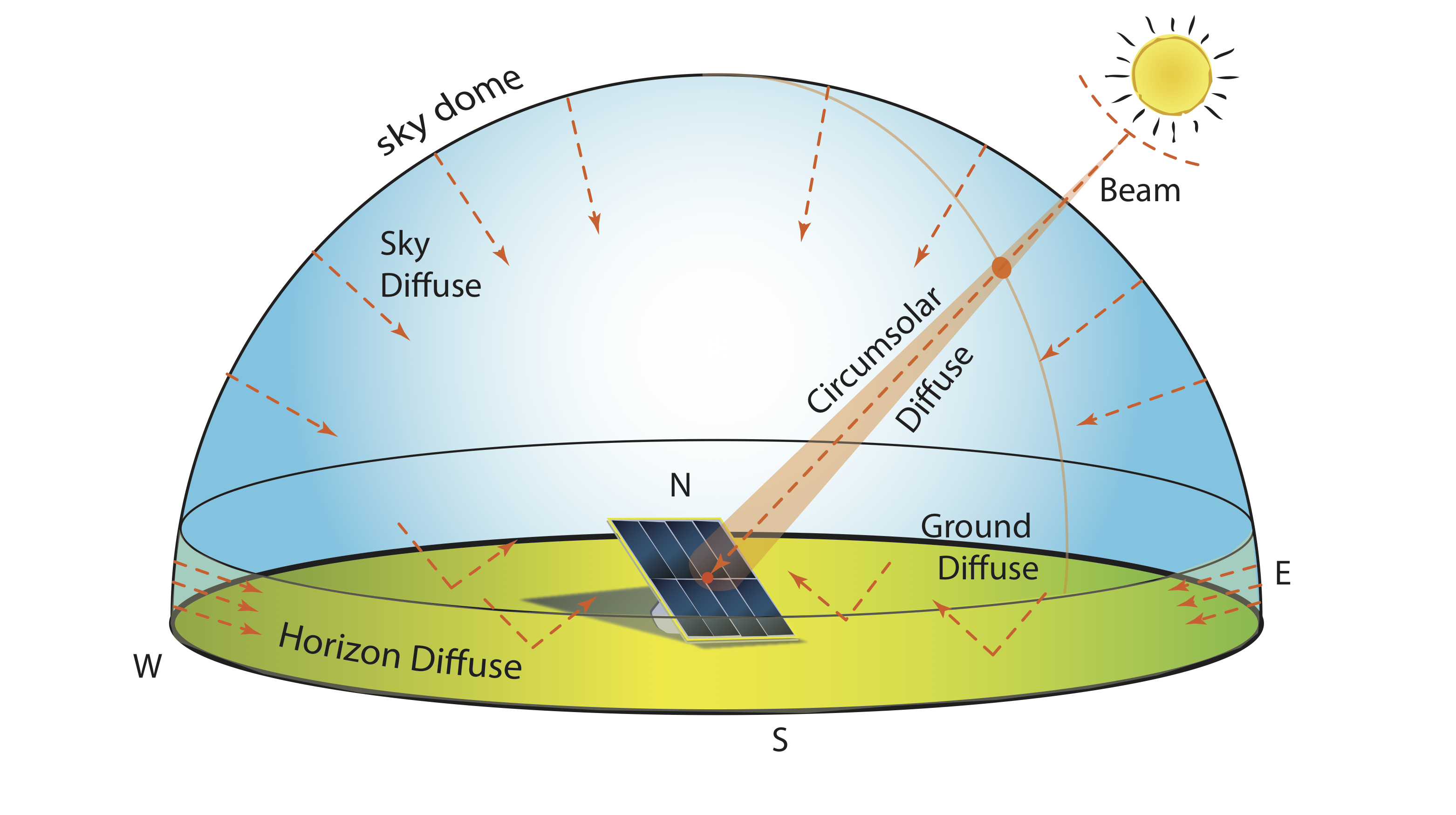
The Flow of Data from GHI to components to POA
In the following flow chart of data processing, we see that measured irradiance (shortwave, from the Sun) is measured in four typical manners:
- GHI (global horizontal irradiance), then integrated to the desired time step (1 min, 5 min, 1 hour)
- DNI (direct normal irradiance), not the same as beam horizontal irradiance (Gb) or beam tilted irradiance (Gb,t)
- DHI (diffuse horizontal irradiance), using a shadow band or similar device to obscure the beam component
- POA (plane of array irradiance), then integrated to the desired time step

In the figure, we have integrated the time step to 1 hour of irradiation on a horizontal and tilted surface, respectively: I and It.
Measurement 1 (GHI) is the most common for a local site assessment in SECS design. Equipment for measuring DNI and DHI are atypical in an application site where the initial site assessment is beginning, and are absent from our satellite maps of the solar resource. Measurement 4 (POA) is becoming more and more popular, as it can potentially remove several steps of error propagation from empirical correlation on site.
Looking across the top line (Measurement 1), we see that we must perform "empirical correlations" using a metric called an "hourly clearness index" (kT) to arrive at "calculated horizontal components of Ib and Id (beam and diffuse hourly irradiation). Then, we must apply an "anisotropic diffuse sky/ground model" and sum the tilted components of irradiation, to finally arrive at a calculated POA irradiation estimate.
Paths 2 and 3 add to the level of precision by stepping past the clearness index correlations (which is error-prone) before applying an anisotropic diffuse sky/ground model and summing to a new calculated POA estimate.
Path 4 skips all of the empirical models and directly measures and integrates the irradiation on a POA surface. The one additional benefit would be to have a DNI measure along with a POA measure, for component decomposition if necessary (required for windows, for example).
4.5 Decoupling Beam and Diffuse: Clearness and Clear Sky Indices
Reading Assignment
- J.R. Brownson, Solar Energy Conversion Systems (SECS), Chapter 8: Measure & Estimation of the Solar Resource (Focus on Empirical Correlation for Components.)
- Reindl, Beckman, and Duffie (1990) Diffuse Fraction Correlations [105]. Solar Energy J. 45(1) 1-7.
- [repeated] C. A. Gueymard (2008) From Global Horizontal to Global Tilted Irradiance: How accurate are solar energy engineering predictions in practice? [106] Solar 2008 Conference, San Diego, CA, American Solar Energy Society
- Optional: Liu and Jordan (1960) The Interrelationship and Characteristic Distribution of Direct, Diffuse, and Total Solar Radiation [109]. Solar Energy J. 4(3), 1–19.
Please make sure you read all of Ch 8 in SECS for this lesson, again maintaining focus on the same section "Empirical Correlation for Components" and this page content. In the two additional readings, it is OK to scan the Reindl et al. paper and the Gueymard paper for key elements that are parallel with the page content.
System designers do not always have the benefit of designing SECS with horizontal surfaces. Many times, these surfaces are tilted at various angles and have various orientations. In such situations, designers and engineers must make estimations for tilted surfaces based on data for horizontal surfaces.
In order to estimate, we first have to break apart the beam horizontal component from the diffuse horizontal components. This has been achieved historically by a methodology established in the 1950s and 60s by Profs. Ben Liu and Richard Jordan (our supplemental reading that is included to add context and the entire line of research that has been applied from then until now).
The availability of solar data is very important when calculating the amount of radiation incident on a collector. Engineers and designers commonly make use of average hourly, daily, and monthly local data. However, the most common measurement available is the Global Horizontal Irradiance (GHI), which is then integrated through a data logger into hourly irradiation, or minute irradiation.
Estimation is an effective tool that involves the use of empirical models that were developed over the last 4-5 decades. The only tools we need are the equations for calculating hourly and daily extraterrestrial irradiance (Air Mass Zero, or AM0) and the integrated energy density (J/m2) gathered from a horizontally mounted pyranometer. These empirical methods to decouple beam and diffuse horizontal components are termed Liu and Jordan transformations, after the initial paper in 1960.
The Clearness Index
The linkage between the two data for horizontal orientation are the clearness indices (kT, KT, and ). This index is simply a measure of the ratio of measured irradiation in a locale relative to the extraterrestrial irradiation calculated (AMo) at the given locale.
- : the hourly clearness index for Total or global irradiation (that's what the "T" is for). This is a ratio of measured energy density against energy density for extraterrestrial solar in one hour.
- : the daily clearness index for Total irradiation. This is a ratio of measured energy density against energy density for extraterrestrial solar in one day.
- : the monthly average daily clearness index for Total irradiation. This is a ratio of measured energy density averaged over the month as one day, against the energy density for extraterrestrial solar for an average day.
For KT →1: atmosphere is clear. For KT →0: atmosphere is cloudy. However, this measure incorporates both light scattering and light absorption. Keep in mind that a fraction is not a percentage, and in our case for a cumulative distribution, it is a decimal value between 0--1.
The Clear Sky Index
There is also an alternate indicator for the way that the atmosphere attenuates light on an hour to hour or day to day basis. This is the "clear sky index" (kc). Mathematically, the clear sky index is defined as
and it has been proposed that 1-kc is a very good indicator of the degree of "cloudiness" in the sky.
So, why do we use either the clearness index or the clear sky index? The answer at the moment is persistence. While it is likely that the clear sky index is more useful than the older clearness index in the long term, all the core research for the empirical calculations used in softwares like TRNSYS, Energy+, and SAM was based on kT.
The Historical Backdrop: the Clearness Index
In the 1960s, Liu and Jordan found that for different US locations with the same value of , the cumulative distribution curves of KT were identical, almost irrespective of latitude and elevation.\marginnote{A cumulative distribution describes the frequency or fraction of occurrence of days in the month below a given daily clearness index, KT}. This work was expanded into equations by Bendt et al.,\cite{Bendt81} using 20 years of real measurements in 90 locations in the USA. However, it was determined that the data sets were not so similar from region to region (e.g., the tropics had different correlations than the temperate USA, India was different from Africa, etc.) This work was followed by Hawas and Muneer for India and Lloyd for the UK, among others.\cite{Hawas85,Lloyd82}
Remember this! KT distributions are not universal---they are regional and empirically derived. For all of our future work, we will only rely on hourly kT values, and the manner in which kT is used to back out a value of Ib, the hourly beam irradiation component on a horizontal surface.
Self-Check
4.6 Using Components for a Tilted Aperture
Reading Assignment
- J.R. Brownson, Solar Energy Conversion Systems (SECS), Chapter 8: Measure & Estimation of the Solar Resource (Isotropic and Anisotropic Sky Models.)
- [repeated] C. A. Gueymard (2008) From Global Horizontal to Global Tilted Irradiance: How accurate are solar energy engineering predictions in practice? [106] Solar 2008 Conference, San Diego, CA, American Solar Energy Society
Please make sure you read all of Ch 8 in SECS for this lesson, still related to "Empirical Correlation for Components," but paying attention to the isotropic and anisotropic sky models and this page content. This is the third page for which we have included a review of the Gueymard paper, so you should be familiar with the findings by now. The Perez et al. paper will be useful to you in Learning Activity 4.2 and for your Lesson Quiz.
Earlier, we discussed the different components of light, beam and diffuse on a horizontal surface. Now, we will discuss how these components can be estimated for tilted surfaces through isotropic or anisotropic diffuse sky/ground models of light source components.
Estimating the Plane of Array (tilted surfaces)
We shall see that we do not need to measure every component of light (scattered and unscattered) to make estimations on the contributions of each component to the total irradiation incident on the aperture of interest. We can rely somewhat on decades of historical observation and empirical correlation by solar scientists and engineers for hourly, daily, and monthly average day data.
The main tools we need are the equations for hourly and daily extraterrestrial irradiance (Air Mass Zero, or AM0) and the integrated energy density (irradiation: $MJ/m^2$) gathered from a horizontally mounted pyranometer, which you learned of in the last section. We shall also find that we can infer more than just the components of light from the ratios of measured irradiation to AM0 calculated irradiation--we can describe the fractions of days in a given month where lighting conditions will be clear or overcast/cloudy.
Following our step to break apart the beam horizontal component from the diffuse horizontal components, we then estimate the components on a tilted surface.
Procedure for Components
For a tilted plane of array,
Total Radiation = beam + diffuse, sky + diffuse, ground
A simple calculation of the beam component can be achieved using
Radiation on a sloped surface can be calculated for the beam component of irradiation by the geometric scaling factor of
In order to estimate the diffuse component, we use alternate models that become increasingly better fits with the empirical data. We can integrate any of these equations over an hour or a day (irradiation). I prefer to offer the irradiance version as a bit easier to read. Note: all of these estimation models use irradiation values that were measured from a pyranometer mounted along the horizontal plane, and then estimated for beam and diffuse components from data correlation or directly measured using a shadow band measurement and energy balance equations.
Isotropic Diffuse Model: Liu & Jordan (1960)
The isotropic sky model was developed in the 1960s to estimate the diffuse sky on a tilted surface, complemented by an estimate for diffuse light from the ground. This model assumes that the sky is uniform in composition across the sky dome.
The following expression gives the total solar irradiance incident on a tilted surface as
where,
The fraction proportional to the collector tilt is called the diffuse sky irradiance tilt factor for an isotropic sky model, and the reflectance of the ground is called the albedo (a fraction between 0 and 1), and is multiplied by the GHI and the diffuse ground irradiance tilt factor for an isotropic sky model.
Note: "Surface": the aperture. : is the collective reflectivity of the ground (the albedo). reduces the irradiance G by a value between 0--1. On an inclined surface, Gd,ground increases, relative to a horizontal collector.
HDKR Model:
This model incorporates isotropic diffuse, circumsolar radiation and horizontal brightening. It also employs an anisotropic index A defined mathematically as
The total irradiance on a tilted surface is then calculated by using
Go to Kalogirou (Solar Energy Engineering) Ch 2 (pdf from Library) this will be labeled the "Reindl model"
Perez Diffuse Model: Richard Perez (1990)
This is an anisotropic diffuse sky model that takes into consideration the real observations of subcomponents of diffuse light. The Perez model adds the circumsolar diffuse component and the horizon diffuse component to the diffuse$_{sky}$ component of the isotropic model. Notice how the beam component is not mentioned here--it doesn't change.
Sidenote: Richard Perez is a Senior Research Associate in the Atmospheric Sciences Research Center in SUNY Albany. He has a great website [122].
The shape factors (F) in this model can be reviewed in the original article by Perez et. al (1990). However, we can inspect the equations and observe in the equation that $F_{surface-sky}$ is reduced by a proportion of $F_1$ (circumsolar radiance), and $F_2$ can either increase or decrease the contribution of horizon radiance.
Try This! Tilted Surface Radiation Model
Software: SAM from NREL- You can open up SAM [37] at this point and click the button "Create a New File."
- Click on "Photovoltaics (Detailed)" on the left of the pop-up window ("Choose a performance model").
- Click on "Residential (Distributed)" on the right of the pop-up window ("then choose from the available financial models").
- Hit "OK."
- You will now have a default residential PV project, based in Phoenix, AZ. There will likely be a SunPower (California company) PV module, and an SMA America dc-ac power inverter listed on the left column of shortcut tabs. They're not really "tabs" like the tab at the top of the window, but I'm going to use that term for convenience in the class.
- Click on the shortcut tab called "Location and Resource" (will list "Location," latitude ($\phi$), longitude ($\lambda$), and elevation above sea level in the shortcut.
- At the bottom of the screen on the right is a large "+" sign labeled "PV Albedo and Radiation". Please expand the section. I want to draw your attention to the little section called "Diffuse Sky Model (Advanced)." Yep, it's so advanced that you don't even realize this is where a powerful data transformation sits!
You can see that one may select "Irradiance Components used for Calculation": this is specifying the type of horizontal irradiation components that you will use in your tilted model. In a data set called the Typical Meteorological Year, the data for the beam is often not actually a measured value.
You can also see that one may select three diffuse sky/ground transposition models to transform the "Irradiance Components" (horizontal) to tilted values. The default is the Perez model that we describe below (and in your supplemental reading). The isotropic model is not used in practice, but it contains the basis for the other anisotropic models of Hay-Davies-Klutcher-Reindl (HDKR) and Perez et al. 1990.
Diffuse Sky Model (Advanced)
- Tiny box hidden within a plus sign, whole lotta power. Keep that in mind.
- Also, when in doubt: Read the Fine Manual. SAM has a detailed Help manual with links to the literature for every aspect of the program.
Optional Reading
- Perez, Ineichen, and Seals (1990) Modeling Daylight Availability and Irradiance Components from Direct and Global Irradiance [112]. Solar Energy J. 44(5), 271-289.
References:
Liu, B.Y.H., Jordan, R.C., 1960. The interrelationship and characteristic distribution of direct, diffuse, and total solar radiation. Solar Energy 4(3),1-19
Perez, R., Ineichen, P., Seals, R., Michalsky, J., Stewart, R., 1990. Modeling daylight and Irradiance components from direct and global irradiance. Solar Energy 44(5), 271-289
4.7 Typical Meteorological Years: A Mosaic of Data
Reading Assignment
- J.R. Brownson, Solar Energy Conversion Systems (SECS), Chapter 8: Measure & Estimation of the Solar Resource (Focus on Meteorological Years: Collage of Data.)
- Kalogirou, S. (2011) Ch 2 (section 2.4.1-2.4.2) pp 106-117. Typical Meteorological Year [available on eReserves]
Your reading in Ch 8 of SECS will introduce the concept of Meteorological Years, while the Ch 2 reading in Kalogirou offers a condensed description of how a TMY data set is formed and how the files are formatted. The Supplemental readings address the most recent version of the TMY data sets in the USA (TMY3), and point to the National Solar Radiation Database maintained by NREL.
The data that you will find in your SAM simulation software, and the data that is all over the web in resources like the NREL Dynamic Maps of the USA solar resource [123], come from a single database, called the NSRDB, or the National Solar Radiation Database. There are currently three generations of TMY.
What is a Typical Meteorological Year? Why would we use a synthesized year of data for solar resource simulations?
A typical meteorological year (TMY) data set provides designers and other users with a reasonably sized annual data set that holds hourly meteorological values that typify conditions at a specific location over a longer period of time, such as 30 years. TMY data sets are widely used by building designers and others for modeling renewable energy conversion systems. Although not designed to provide meteorological extremes, TMY data have natural diurnal and seasonal variations and represent a year of typical climatic conditions for a location. The TMY should not be used to predict weather for a particular period of time, nor is it an appropriate basis for evaluating real-time energy production or efficiencies for building design applications or solar conversion systems.
...The TMY data set is composed of 12 typical meteorological months (January through December) that are concatenated essentially without modification to form a single year with a serially complete data record for primary measurements. These monthly data sets contain actual time-series meteorological measurements and modeled solar values, although some hourly records may contain filled or interpolated data for periods when original observations are missing from the data archive.
Wilcox and Marion (2008) NREL/TP-581-43156
Estimation can often be evaluated relative to 30 year averages of weather conditions at specific locations, termed the Typical Meteorological Year (TMY). These data are not reasonable estimates of extreme conditions (e.g., hurricanes, tornadoes) and may also be inaccurate for evaluating site or time-specific data. The most common database is TMY3, now collected from the period of 1991 to 2010.
TMY data was initially developed to aid in building simulation, for modeling the energy demands in counterpoint with the solar/meteorological gains. As in your software SAM (and the source code, TRNSYS), TMY is also used by SECS design teams for initial estimates of energy and financial returns on investment. We can use SAM's TMY data set to evaluate PV, solar hot water, and CSP systems.
The source data for the TMY set in the USA comes from the NSRDB, or the National Solar Radiation Database.
Try This!
SAM Location and Resource HelpLet's go back to the SAM software and explore the solar resource data in its browser.
- You can open up SAM [37] at this point and click the button "Start a new project"
- Click on "Photovoltaics (Detailed)" on the left of the pop-up window ("Choose a performance model").
- Click on "Residential (Distributed)" on the right of the pop-up window ("then choose from the available financial models").
- Hit "OK."
- You will now have a default residential PV project, based in Phoenix, AZ. There will likely be a SunPower (California company) PV module, and an SMA America dc-ac power inverter listed on the left column of shortcut tabs. They're not really "tabs" like the tab at the top of the window, but I'm going to use that term for convenience in the class.
- Click on the shortcut tab called "Location and Resource" (will list "Location," latitude ($\phi$), longitude ($\lambda$), and elevation above sea level in the shortcut.
- Leave the location on Phoenix.tm2 and look inside the section "Tools."
- Click the button "View hourly data...," and a new window will pop up.
Reminder: This information will be used when you create your final project.
Optional Reading
- S. Wilcox and W. Marion (2008) Users Manual for TMY3 Data Sets [110]. NREL/TP-581-43156
- S. Wilcox (2012) National solar radiation database 1991- 2010 update: User’s manual [111]. NREL/TP- 5500-54824
- National Solar Radiation Database website (NSRDB [124])
4.8. Discussion Activity
Lesson 4 Discussion in Yellowdig!
We have just read about Typical Meteorological Years (TMY) as simulation inputs in beginning project assessment. I want you to consider the positive and negative attributes of TMY data sets in terms of project design and then in terms of project operation and management. Post your answers to the following questions, and then let's have a discussion about them.
Here are some guiding questions:
- What is the advantage in using TMY data in project development?
- Why do we only have "one year" of mosaicked data?
- What are the cautions and limitations in using TMY data?
Tagging
When you create a post in the Yellowdig discussion space, you are required to choose a topic tag. For Lesson 4 discussions, please use these tags:
You can tag your post with one or several topics at the same time. All posts and contributions you create are added up to one score at the end of the week.
Importance of interaction
Yellowdig tip: remember to check in the Yellowdig site often - it is much easier to aborb the posted information in bits rather than reading multiple posts and comments in a bulk. Click to "Home" icon - you will be able to see all the unread posts in one place.
Grading
Yellowdig points you earn over the weekly point earning period (from Saturday to next Friday) will count towards 1000 pts. weekly target. But you can go above it (to 1350 pts. max). Yellowdig discussions will account for 15% of the total grade in the course. Check back the Orientation Yellowdig page in Canvas for more details on the points earning rules.
Deadline
There is no hard deadline for participating in these discussions, but I encourage you to create your posts in the middle of the study week (Sunday) to allow others to engage and respond while we are learning specific topics in the lesson. Also, remember that each weekly point earning cycle ends Friday night, and a new period starts on Saturday.
4.9 Measurement vs Estimation
Reading Assignment
- J.R. Brownson, Solar Energy Conversion Systems (SECS), Chapter 8: Measure & Estimation of the Solar Resource (focus on When Empirical Correlations are not Appropriate.)
- C. Gueymard (2012) Solar Resource Assessment and Forecasting: Recent Achievements, Bankability Pressures, and Current Challenges [108]. (slides) 2012 World Renewable Energy Forum, Denver, CO May 12-17.
- Sengupta et al. (2015) Best Practices Handbook for the Collection and Use of Solar Resource Data for Solar Energy Applications [107]. NREL/TP-5D00-63112: p. 19-62: Chapter 3. Measuring Solar Radiation
Review the linked presentation from solar expert Dr. Chris Gueymard. It provides a historical context of where we came from in solar resource assessment, the current pressures associated with bankability, and the new challenges that we expect in the field in the near future. Now, compare the presentation to your earlier reading of Sengupta et al. (2015). In particular, scan the Chapter 6: Applying Solar Resource Data to Concentrating Solar Power Projects (p. 97).
Finally, go back to your Ch 8 SECS reading, and review the section "When Empirical Correlations are not Appropriate." You may begin to realize where the old empirical methods are useful, and the occasions when they are not useful to project implementation for our stakeholders.
I want you to think about the need for estimation in preparing a new project design using a software like SAM. When does the estimation process give way to more detailed measurements in a SECS project?
Think about where estimated data sets like TMY fit in the process of applying solar resource data detailed below.
- Pre-feasibility
- Feasibility
- Due Diligence
- Project Acceptance and Systems Operation
When do we need to work as a larger design team with solar resource specialists who can monitor a site actively and maintain the equipment? When is the investment in measurement equipment appropriate for the planned project? For solar incorporations on the facade of a building (roof, windows, walls), do we need to measure the solar resource at the site?
As the world looks for low-carbon sources of energy, solar power stands out as the most abundant energy resource. Harnessing this energy is the challenge for this century. Photovoltaics and concentrating solar power (CSP) are two primary forms of electricity generation using sunlight. These use different technologies, collect different fractions of the solar resource, and have different siting and production capabilities. Although PV systems are most often deployed as distributed generation sources, CSP systems favor large, centrally located systems. Accordingly, large CSP systems require a substantial investment, sometimes exceeding $1 billion in construction costs. Before such a project is undertaken, the best possible information about the quality and reliability of the fuel source must be made available. That is, project developers need to have reliable data about the solar resource available at specific locations to predict the daily and annual performance of a proposed CSP plant. Without these data, no financial analysis is possible. This handbook presents detailed information about solar resource data and the resulting data products needed for each stage of the project."
--Tom Stoffel, Dave Renné, Daryl Myers, Steve Wilcox, Manajit Sengupta, Ray George, Craig Turchi; NREL/TP-550-47465
4.10 Learning Activity: Clearness Index
The purpose of this activity is to learn how the clearness index ( ) can be determined for a specific day and time based on collected meteorological data and knowledge of the extraterrestrial solar irradiance. By definition, is essentially the attenuation factor of the atmosphere, showing the ratio between the solar radiation incoming into the Earth atmosphere and that reaching the ground:
where is the energy density measured at the horizontal surface at a locale, and is the energy density just outside the Earth’s atmosphere at AM0. Of course, there are multiple natural phenomena that are responsible for scattering and reflection losses.
The clearness index was developed by the researchers Liu and Jordan at the University of Minnesota in the 1960s, and to this day this metric is still used by various models and empirical correlations for quantifying components of solar light.
In this activity, you will need to calculate the hourly values for two different hours on July 31st, 2007 at Penn State SURFRAD location (Rock Springs). This activity builds upon irradiance data you were treating in Lesson 3, so you will use the same SURFRAD file for the clearness index calculations.
Part 1. Calculation of hourly irradiation (I) from SURFRAD data
Extract GHI data from the SURFRAD file (Penn State location) for July 31st, 2007 for two different hours: (a) 8-9 am and (b) 1-2 pm.
Convert GHI data (measured in ) to energy density values (in ) by multiplying them by time. Note: SURFRAD data are recorded at 3 min step.
Find the total solar energy density (irradiation) delivered per square meter over each hour period. This is the measured value. Present your results in .
Part 2. Calculation of the extraterrestrial irradiation (Io)
- Calculate the hourly extraterrestrial GHI (AM0) for each of the hours of 8-9 am and 1-2 pm hours on July 31, 2007 using the equation below:
\[{I_o} = \frac{{12 \cdot 3600}}{\pi } \cdot {G_{0,n}} \cdot \left[ {\frac{\pi }{{180}}({\omega _2} - {\omega _1})\sin \phi \sin \delta + \cos \phi \cos \delta (\sin {\omega _2} - \sin {\omega _1})} \right]\]
In this equation: is hour angle for hourly endpoints 1 (beginning) and 2 (end); is latitude, is declination for the day of interest, and is normal irradiance at AM0. All these parameters can be taken from the Bird model for State College location you used in Lesson 3. You only need data for day #212 in this calculation. - Present your value in . The results for are expected to be on the order of 0.5-5 . This will provide you with the denominator value in the expression.
Part 3. Calculation of
Plug in your and values into the ratio and obtain values for both 8-9 am and 1-2 pm hours. Your result should be a number between 0 and 1.
Provide a brief discussion of results. What are the reasons for clearness index to change during the day?
Submitting Your Work
Your report should include the following: (a) Data tables with GHI for specific hours (8-9 am and 1-2 pm on 7/31/07) and corresponding irradiation values; (b) hourly energy density in ; (c) calculation of extraterrestrial irradiation shown; (d) hourly extraterrestrial energy density in ; (e) values for each of two hours; (f) brief discussion of the obtained values.
Upload your report file to Canvas (Lesson 4 Learning Activity DropBox) in PDF or docx format.
Grading Criteria
This activity is graded out of 30 points.
| Criteria | Available Points |
|---|---|
| Table of GHI data with corresponding irradiation values
Data for both 8-9 am and 1-2 pm hours |
Up to 5.0 points |
| Correct hourly energy density (irradiation) value is reported (in ) |
Up to 5.0 points |
| Calculation of the extraterrestrial energy density is shown and steps are explained |
Up to 5.0 points |
| Correct extraterrestrial energy density is reported (in ) |
Up to 5.0 points |
| Clearness index is calculated for both 8-9 am and 1-2 pm hours |
Up to 5.0 points |
| Discussion of the results is provided |
Up to 5.0 points |
Deadline
See the Calendar tab in Canvas for specific due dates.
4.11 Summary and Final Tasks
You have reached the end of Lesson 4!
This was the last of four lessons wrapping up the arc of core solar resource assessment content. In Lesson 4, you were introduced to the key elements of the solar resource and the ways we measure or estimate the resource in a given locale. We built upon our knowledge from Lessons 2 and 3, and also drew some content in a Lesson 3 activity to be applied in a Lesson 4 activity.
You went through a detailed reading on Best Practices for Solar Collection and Use to start, which provided us with a good amount of information for both CSP and non-CSP practices too. There were elements in the reading that stressed the importance in finding the appropriate data set for a SECS development plan. Solar resources are important to residential and commercial buildings, as well as to PV arrays, as well as to utility scale CSP and solar hot water or steam applications. Your job is to be aware of the type of data you use, to know the transformations that are done to the data to turn it into a useful input (for simulation), and to develop levels of confidence in using various qualities of data as a practitioner.
Now that you have completed the lesson, you should be able to:
- explain why the human eye is a poor solar detector and creates bias in decision making;
- describe the equipment used to measure irradiance and irradiation in the field and from space;
- contrast collecting data for horizontal irradiance and DNI with (Plane of Array) POA measurements;
- describe the meaning of a component of light, and list the components for anisotropic skies on a tilted surface;
- explain scenarios where direct POA (Plane of Array) measurement is not available and one must use empirical correlations (via clearness indices) to estimate irradiation on a horizontal surface;
- understand and be able to apply typical meteorologic year (TMY) data to energy system simulations.
You can always go back to these readings and dig into the references. There is now extensive documentation to guide you in your practical development; you just need to reach out and read it!
Reminder - Complete all of the Lesson 4 tasks!
Double-check the to-do list on the Lesson 4 Learning Outcomes page to make sure you have completed all of the activities listed there before you begin Lesson 5.
Lesson 5 - Solar Economic Analysis
5.0 Overview
Overview
OK, we are now out of the deep end of the class and moving into the frameworks for design and valuation of the solar resource. We will be developing a second major arc through Lessons 5, 6, and 7, working through economic and financial issues. So you should see connectivity among these three lessons.
In Lesson 6, we will discuss ways to meet the Goal of Solar Energy Design and Engineering: to maximize the solar utility for a client or group of stakeholders in a given locale. We will dig into a short statement, and find a nearly infinite variety of options for design. But first, we need to find out about our clients or stakeholders as "utility maximizers" in Lesson 5; what makes people demand solar energy products, and how easily will they change their minds? Are there any losses or risks that people are avoiding by choosing solar energy goods and services? Essentially, what are the driving forces for people to adopt solar energy?
Solar Energy Economics helps us to establish the following argument: just because one perceives the solar resource to be weak in a region does not mean that it cannot be successful as a technology in that society. The solar resource is ubiquitous, and we make use of it whether we decide to or not. What is interesting for solar energy is that our raw "product'' is the photon. We apply technologies and skilled effort to convert photons into a diversity of goods that society is interested in purchasing.
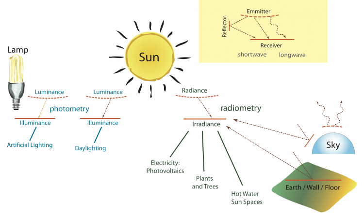
The economics of solar technologies helps us to address why we make decisions to use the Sun. We make use of the Sun throughout our lives, but in solar design, we work to develop compelling arguments to the client to increase their marginal demand for the Sun. There is a sense that energy is somewhere between a product and a good in demand by society, and it must be supplied by non-trivial mechanisms, at some cost for the exchange of goods. In order to make marginally (or incrementally) more use of the Sun, we have to learn about the skills to measure and predict the variable phenomenological behavior of solar irradiance as well as the dependence of the variable irradiance on the location of the client in question.
5.1 Learning Outcomes
By the end of this lesson, you should be able to:
- identify the key features of supply and demand for energy systems;
- list the two general motives that shift the value of any commodity;
- list the three specific drivers that will affect the valuation of light as a quantified mineral reserve;
- list the four main factors affecting the price elasticity of demand;
- describe the hypothesis of the energy constraint response for solar energy.
What is due for Lesson 5?
This lesson will take us one week to complete. Please refer to the Course Syllabus for specific time frames and due dates. Specific directions for the assignment below can be found within this lesson.
| Required Reading: |
J.R. Brownson, Solar Energy Conversion Systems (SECS), Chapter 9 - Solar Economics Selected readings from EBF 200 course |
|---|---|
| Optional Reading (not required): | G. Mankiw Principles of Economics [127]. This might be a nice resource for your future study but is not required for this course. |
| To Do |
Discussion 1: Light as a mineral resource Discussion 2: Hypothesis of Energy Constraint |
| Topic(s) | Supply and Demand Light as a solar reserve Price elasticity of demand A hypothesis of the Energy Constraint Response |
Questions?
If you have any questions, please post them to the Lesson 5 General Questions and Comments Discussion Forum in Yellowdig. I will check the forum regularly to respond. While you are in a discussion, feel free to post your own responses if you, too, are able to help out a classmate.
5.2 Supply and Demand of Energy
Reading Assignment
We start with the material on solar economics in the Brownson's book:
- J.R. Brownson, Solar Energy Conversion Systems (SECS), Chapter 9: Solar Energy Economics (Focus on the Introduction and Flows and Stocks.)
Then I would like you browse through a few pages from anoter course: EBF 200: Introduction to the Energy and Earth Sciences Economics:
- EBF 200: What is Economics? [128] (Review the concepts of Goods, Scarcity, and Tradeoffs)
- EBF 200: Utility and Individual Rationality [129] (Understand Consumers as Utility Maximizers)
- EBF 200: Supply and Demand [130] (Review the basic economic concepts)
As a refresher on energy terms and definition, please refer to this website (see "What is Energy?" link).
- Energy Information Administration Energy Explained [1]
When we deal with goods and services tied to energy systems, things get pretty interesting! When you think about energy and natural resources, the tendency in energy economics is to think mainly of "non-renewable resources" or exhaustible resources like coal/oil/natural gas, etc. I want you to think about how much of our social economic perspective on energy is based on exhaustible resources.
We want to better understand why our clients and stakeholders (or even we) make decisions to adopt technologies that deliver goods and services from the Sun. The form of energy is radiant, from a Solar resource system, and we transform radiant energy into other useful forms to do work.
Energy Supply and Demand
The readily accessible energy that can be used to "do work" in society is still considered a limited natural resource, or good. In economic terms, we would say that many of our useful energy goods are scarce.
As we read in EBF 200, "What is Economics?" Prof. Gregory Mankiw lists seven microeconomic principles. Recall that microeconomics refers to individual economic actors considered as people and firms and their corresponding interactions in markets.
- People face tradeoffs.
- The cost of something is what you give up to get it.
- Rational people think at the margin.
(Watch the following YouTube video of Thinking at the Margin by Prof. Mario Villarreal-Diaz.)
Video: CHAPTER # 2 THINKING AT THE MARGIN (5:26)
MARIO VILLARREAL-DIAZ: Individuals make choices and tradeoffs based on comparisons. When they are trying to decide what is the best choice, depends on those comparisons. One alternative versus the other. Let's think about ordering some fast food.
If you go to a restaurant, and they have the combo number one, and the combo number one includes a hamburger and some French fries, and the price is 10 dollars, then you can take a look at the combo number two. And the combo number two includes the hamburger and the fries and a milkshake. And it's 13 dollars.
So, immediately when you think about it, you say, well, what am I going to get from those extra 3 dollars? A milkshake. So, that extra unit of food is going to cost me 3 dollars. So, the question you are trying to answer is, is that milkshake worth 3 dollars for me or not?
And then, you make your choice. You make your decision of combo number one versus combo number two. That's thinking at the margin. At the margin means to think about the next increment, the next unit. That relatively small change, the net addition or subtraction when I make a choice.
Marginal thinking helps us understanding puzzles such as why diamonds are so much more expensive than water, given that water is indispensable and essential for life. And the answer is that the marginal utility of water compared to the marginal utility of diamonds decreases way faster.
Think about the first glass of water if you're thirsty-- very satisfying. Think about the second one. Think about the 20th or 50th glasses of water. Maybe you will be not that happy with getting that 50th glass of water. And now think about diamonds. What is the marginal utility of that extra unit of diamonds?
Probably will not decrease at all. Probably will even increase. What I'm trying to say here is that if you compare the value of the extra unit of water versus the value of the extra unit of diamonds, it is obvious why diamonds are much more expensive than water.
Individuals make choices at the margin all the time. This is part of the way we think, even though we don't notice. But not only individual decisions such as buying combo number one or combo number two are made thinking at the margin. Businesses also make decisions with this way of thinking.
For example, if a business wants to hire an extra employee, they think exactly about the same way. How much is it going to cost me, that extra employee? Well, it's going to cost me his or her salary. Well, now we need to compare it versus what? How much he's going to produce.
What is going to be the value added for having an extra employee? What is his or her marginal production? And then, of course, if his or her marginal production is larger than how much I'm going to pay his or her marginal cost, then it's a good business decision to hire that extra person.
These basic tools, such as incentives, matter, opportunity cost, and thinking at the margin are not substitute. They complement each other. They are intertwined in the way economists see the world. Thus, when somebody is deciding about the combo one versus the combo two and thinking, should I get the milkshake? That is worth for me three more dollars?
She's not only thinking about that extra pleasure that the milkshake is going to give her, but about the opportunity cost of using those $3 to buy that milkshake. And what is the alternative use of those three dollars? Maybe some popcorn at the movies. Maybe candy at the movies or what have you.
So, at the same time that is thinking at the margin is thinking at the opportunity cost of that money, how to allocate those resources. So, we do that all the time. For a public official, it might be the case that marginal analysis doesn't come that naturally because there is not that attachment.
However, it should. Because still there is an alternative use of those public funds. So, public officials should think, if I allocate these resources in this project, how much I'm going to get out of it? And maybe I'm not going to get enough, and I should invest that money in somewhere else.
- People respond to incentives.
- Trade can make everyone better off.
- Markets are usually a good way to organize economic activity.
- Governments can sometimes improve market outcomes.
In solar systems design, we work to Maximize Solar Utility for the client or stakeholders in a given locale. We will describe the methodologies to do so in the next lesson. But our clients are individuals who are in demand of a solar good. The firms developing or deploying SECSs are supplying access to the solar goods.
- Consumers (clients) can be thought of as "Utility Maximizers;" they want to achieve the highest preference for given goods or service.
- Suppliers (designers/engineers/builders) can be thought of as "Profit Maximizers."
Forms of Energy in Demand
Across the planet, there are non-uniform, ever-increasing demands for energy as thermal heat and electrical power. Light, as electromagnetic radiation, is another form of energy, used as well for visual comfort and indoor activities. The photon can be harvested via a solar energy conversion device. To be clear, photons are ephemeral (flows); they are not collected like fuel in a tank (not stocks).
Energy can be described in terms of sources (as in energy re-sources) and in terms of forms (as in energy trans-form-ations). Think of it this way, an energy source is a resource system, from which we appropriate useful resource units in a given form. Energy is neither created nor destroyed, so if the energy is in a less useful form, we must use an Energy Conversion Device (ECD, not a very technical term, but useful here) to transform one form into a more useful form.
- Thermal (heat)
- Radiant (electromagnetic, light)
- Motion (kinetic)
- Electrical (also called power in the industry)
- Chemical
- Nuclear
- Gravitational
Energy scarcity is partially related to the loss of energy quality with successive transformations. Light happens to be an incredibly high quality of energy, which is then transformed into chemical energy by plants (photosynthesis), or into thermal energy by opaque materials, or kinetic energy via wind, or electrical energy via photovoltaics. (Nuclear and gravitational energy are not linked so directly to radiant energy here.)
Our society is used to beginning with "concentrated sunshine" (geofuels from stored photosynthesis in coal, oil, and gas), and then transforming the chemical form to the thermal form (hot steam), which is then transformed into the motion form (to spin a turbine-generator) and finally transformed into electrical energy.
Sidenote on Heat and Power
The terms Heat and Power have been adopted by several industries to have a specialized trade meaning.
- Power is electrical energy (as opposed to a rate of energy use), and
- Heat is thermal energy (as opposed to the transfer of energy).
Thus, in the energy industry, we hear about Combined Heat and Power (CHP) for energy conversion systems that provide two useful forms in one system.
Self-Check
Optional Reading on Energy Economics
Optional: G. Mankiw Principles of Economics [133]. This might be a nice resource for your future study but is not required for this course.
5.3 Value and Quantity of Light as a Commodity
Reading Assignment
- J.R. Brownson, Solar Energy Conversion Systems (SECS), Chapter 9: Solar Energy Economics (Focus on The Value, Reserve, and Elasticity of Light.)
- USGS Mineral Commodity Summaries (See Appendix C: Reserves and Resources. [134])
- D. Meadows, Thinking in Systems: A Primer, pp 1-9, Bathtubs 101 [135]
We want to focus on how the resource units like electricity, heat, daylight, and money derived from SECS have an elasticity of demand. How do we value the products of light, or how do we even value the solar resource itself as an energy reserve? In our reading, we find that sunlight can be analyzed similarly to a mineral reserve like copper ore.
Our decision to choose solar technologies often depends on the value that we place on light and the value of the resource units derived from shortwave light. You are going to need to think about light as a commodity, or a good that is interchangeable with other goods/services. This is a bit abstract, so take some time to reflect at the end of the page.
Flow vs. Stock Energy Reserves
Stocks and flows exist in nature and in society. We see stocks in business. In nature, a lake is a stock of water, with a river flowing into it. And the Sun is a stock of nuclear fusion yielding a flow of radiant energy.
- Potential: a driving force for flow.
- Flow: a dynamic entity connected to a stock that either supplies or depletes the stock; can be a change in mass, energy, or information with respect to time.
- Stock: an entity that has accumulated over time due to flows; can be stored potential, or a resource system that replenishes itself (like the fusion in the Sun).
- Resource system: often an environmental stock (and could be a human institution).
- Resource units: the flow of a useful resource that a client may appropriate from a resource system.
A resource system is considered renewable if the rate of withdrawal from the stock does not exceed the rate of resource replenishment. In the case of shortwave light, the solar resource system has physical conditions that define an upper limit of flow without disturbing or harming the constitution of the stock. We can't really withdraw sunlight at a faster rate than it comes to us. Hence, sunlight is flow-limited.
A resource system is considered non-renewable if the rate of withdrawal from the stock exceeds the rate of resource replenishment. In the case of geofuels, the process to make them takes 10s-100s of millions of years (and heat/pressure underground), yet the rate of withdrawal can be almost as fast as we want. Hence, geofuels are stock-limited.
The "Quantity" of Light
Compared to what is available on Mars, the quantity of light is abundant on Earth! Even between the Arctic Circles (), there is a great abundance of light available to society to do work. As a society, we are not as skilled at transforming light into useful work as we are at transforming fuel into useful work. We are still struggling to frame light as a valued good, especially as it is all around us every day. So, let's take a look at that value structure.
The value of light from the Sun is variable. There is "less" of an energetic resource from the Sun in the annual irradiation budget for Germany than in the US state of Georgia, yet the value of solar power (as electricity) is much higher in Germany than in Georgia. So is the value of the light to the clients relative to the "quantity" of light, or relative to other parameters.
In the mineral economics of commodity goods, the value of the resource units will vary with respect to two general driving forces:
- demand for the good or service, and
- cost of alternatives.
If the demand for a good goes up, the value of the resource units will go up. If the cost of an alternative good goes up (like the price of geofuels), then the value of the resource units (like solar) will go up.
Light as a Mineral Resource (Commodity)
An increased demand for a mineral commodity will increase the value, and a high cost of alternative goods will increase the value.
Value and quantity are joint properties here. As such, the "quantity" of a mineral reserve can expand or shrink in response to three main pressures. Solar resources follow the same commodity trend. In the case of the solar resource framed as a type of mineral reserve, the solar reserve is available when it is economically feasible, expanding and contracting in response to the following three pressures. That is to say, there are three levels that open up, or expand, the solar reserve in a given locale.
The value of an unconverted photon is a variable quantity, much like the value of a mineral resource in a geologic formation. Once again, the value of any commodity varies with the demand for the good and the costs of alternatives. The three main drivers that affect the valuation of light as quantified mineral reserve are:
- increased demand by clients seeking to avoid fuel costs (choosing an alternative to fuel);
- technological advances that reduce materials costs and/or installation costs;
- presence of incentives (often government incentives).
Let us compare the way in which light is valued with the way that a metal ore (in this case, zinc) is valued. An ore is an unrefined rock composed of minerals, which contains a raw metal that is valued, but which must be processed to access that metal. In our reading from the USGS Commodity Statistics [136], Appendix C, we see that an entire lexicon has been developed for classifying mineral resources. (This site as a whole is also an excellent public resource for evaluating mineral reserves from the US perspective.) We have since classified geofuels as "minerals" in the commodity perspective. So, why not extend the concept outward to the commodity of light, and the derived goods and services?
The following terms are within the textbook reading, and were developed from the U.S. Geological Survey Circular 831, Principles of a Resource/Reserve Classification for Minerals (1980). Note the difference among a resource, a reserve base, and a reserve.
- Resource: material or energy source occurring natively in or on the Earth, with a form, concentration, and quantity such that economic collection and/or conversion of that commodity is currently or potentially feasible. (We could apply this to light, right?)
- Identified Resources: specific resources where the location, grade, quality, and quantity are known from specific meteorological evidence, or where the resource has been estimated. Identified solar resources encompass regions that are economic, marginally economic, and sub-economic. As a reflection of the degrees of meteorological confidence, the economic divisions can be subdivided into components of measured, indicated, and inferred.
- Reserve Base: an identified resource meeting minimum criteria related to a specified solar energy conversion technology practice currently employed to convert to useful work.
- Reserve: the portion of the reserve base that can be economically converted at the time of determination (the locale).
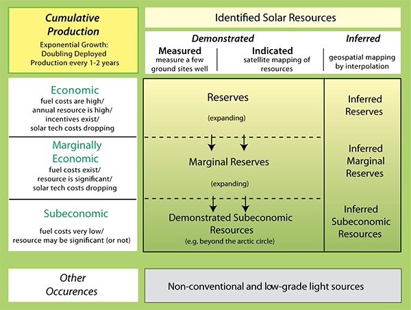
A table shows a two-axis categorical relationship between knowledge of the solar resource and the ability to economically exploit the resource.
On the first axis, three categories describe decreasing levels of knowledge of the resource: “Measured” (measure a few ground sites well), “Indicated” (satellite mapping of resources) and “Inferred” (geospatial mapping by interpolation). The combination of Measured and Indicated resources are termed “Demonstrated,” while all three categories together are termed “Identified Solar Resources.”
The second axis also contains three categories, which describe decreasing levels of economic return from the resource. “Economic” resources are described with the terms: fuel costs are high/annual resource is high/incentives exist/solar tech costs dropping. “Marginally Economic” resources are described with: fuel costs exist/resource is significant/solar tech costs dropping. “Subeconomic” resources can be described by: fuel costs very low/resource may be significant (or not).
Intersections between these category axes are described with text labels. Reserves are shown at the intersection of Demonstrated and Economic resources, while Inferred and Economic resources are termed Inferred Reserves. Marginal Reserves and Inferred Marginal Reserves occur for Marginally Economic resources that are Demonstrated and Inferred, respectively. Demonstrated Subeconomic Resources and Inferred Subeconomic Resources are the last two labelled combinations, and are self-explanatory. An example of Demonstrated Subeconomic Resources is given as those occurring beyond the arctic circle. Arrows and text indicate that as the Reserves move from Economic to Marginally Economic to Subeconomic, the reserve base is expanding. A final category of resource is listed separately from the main table with the heading “Other Occurrences,” and lists non-conventional and low-grade light sources.
A final text box is shown separate, but alongside the table, which describes Cumulative Production of the resource as exponential growth with doubling deployed production every 1-2 years.
5.4 Price Elasticity of Demand
Reading Assignment
- J.R. Brownson, Solar Energy Conversion Systems (SECS), Chapter 9: Measure & Estimation of the Solar Resource (Focus on The Value, Reserve, and Elasticity of Light.)
When we are "thinking on the margin," what do we mean? When an incremental change occurs in the price of a SECS or in the alternative price of electricity from the grid, how do we respond? Do we jump in, or do we wait and see?
Elasticity of Demand
In economics, the measured response (in the market) of how the quantity of a product in demand is changed by the incremental change in the price of that product is termed price elasticity of demand. The demand is considered elastic if a small change (like a decrease) in price leads to people demanding more of the product. The demand in considered to be inelastic if a large change (again, a decrease) in price does not lead to people demanding more of the product. The elasticity of demand for solar power will depend on a few general rules, and we will try to contain our examples to solar scenarios for a client or group of stakeholders.
Criteria for Elasticity
The price of PV just changed. What do you do? Do you go out and invest in a PV system for your roof, or do you wait and see? Clients and consumers (us too!) are influenced by several criteria. The four main factors affecting the price elasticity of demand are:
- availability of close substitutes;
- whether the form of energy is a necessity or luxury;
- how large a share of a consumer's income the good will consume; and
- the time horizon over which the change occurs.
First, one evaluates the availability of close substitutes for the particular SECS of interest. If the desired useful energy form or technology has many available close substitutes, then it will be easier for clients/stakeholders to switch among goods for the same desired feature, and the demand will tend to be elastic.
Next, we ask, is the energy form a necessity or a luxury? Our electricity from the coal/nuclear power plant is typically a necessity right (and thus inelastic)? Is there anything about residential PV that seems to be a luxury to families? When did mobile phones stop being a luxury and become a necessity in modern society?
What share of income can an individual or firm (as clients) devote to paying off a loan for solar technologies or directly purchasing a SECS? If a SECS consumes a large share of my income, what tradeoffs will I need to consider (what will I have to give up in return)?
Finally, when making decisions for energy systems, we must consider the time horizon, or the period of evaluation. For energy consumers, when the cost of energy (in dollars per kilowatt-hour, $\$/kWh$) goes up briefly (on the order of hours or days, or for one month) there's not much that they can do to respond. As such, the price elasticity of demand is said to be inelastic for shorter time horizons. In contrast, when the period of evaluation is framed in terms of decades, as is done for PV systems that have productive life cycles of 30-50 years, then the client perspective can shift and become more elastic. When you buy a house, you're in it for the long-term, right? Similar thinking with SECSs.
Video Perspectives
And now for two short perspectives on the Price Elasticity of Demand to complement the reading. Please watch the following two videos: "Episode 16: Elasticity of Demand" by Dr. Mary J. McGlasson, and "Elasticity - Characteristics that determine elasticity" (Dr. McGlasson is an economics faculty at the Chandler-Gilbert Community College.) I want you to think about solar energy and the resource units derived from the conversion of shortwave light.
Video: Episode 16: Elasticity of Demand (9:33)
PRESENTER: There are many types of elasticity. In particular, I'll focus on the price elasticity of demand. Before I get into specific discussion of elasticity, let me ask you a question. If a business wants to generate more revenue, should it raise the price of its product or lower the price of its product?
I ask because I have a friend who runs a children's bookstore, and when she found out that I was an economist, she asked me this question. Well, actually, she asked if she should be giving an educator discount, but what this really meant, was that she wanted to know if she should discount, or lower, her prices.
So, generally, what would you say? Should a business owner increase prices or decrease prices, in order to generate more revenue?
The answer-- as usual-- is, it depends. Think about it. When your local electric company wants to raise more revenue, it will enact a rate increase. Yet, when an airline wants to quickly generate additional revenue, it will cut ticket prices. Which approach is correct? They both are.
Here's the issue. If I raise my prices, I know that quantity demanded, or the willingness to purchase on the part of my consumers, will drop-- that's just the law of demand. But what the law of demand doesn't tell me is how much the quantity demanded will drop.
When I raise my price, will my customers be very sensitive to the price increase? Cutting back a lot on their purchases? This would be bad for me because I'd lose a lot of revenue. But if I raise my price and my customers only buy a little bit less, not reacting too much to the price increase, this is good. I'd see increased overall revenue.
So, the crucial issue here is to find out how sensitive my customers will be to a price change. Elasticity is a measure of sensitivity, or responsiveness, to price. In equation form, the elasticity of demand, or ED, is equal to the percentage change in quantity demanded over the percentage change in price. Because demand exhibits an inverse or negative relationship, elasticity of demand will be a negative number.
I use percentage change to measure elasticity, rather than absolute change. Let me illustrate why.
If I tell you that product price has gone up by $1, this would be the absolute change. Is this a big change or a small change?
It depends. What's the product? More to the point, what was the original price?
Look, say we're talking about a pack of gum. Originally, the price was 1 dollar, now it's 2 dollars. This represents an absolute change of 1 dollar, but is it a big change or a small change? It's actually a pretty big change-- price doubled, or increased, by 100%.
What if we're talking about a textbook, rather than a pack of gum? Originally, the price was 100 dollars, now it's 101 dollars. This is still an absolute change of 1 dollar, but is it a big change or a small change?
In this case, it's a small change. Price has increased by 1%.
Bottom line is, that we need to know not only the dollar amount of the price change, but also, how this compares to where we started.
Now, technically, the formula for elasticity of demand is the percentage change in quantity demanded over the percentage change in price, which can be found by taking the ratio of the difference between the new and the old quantities over the average of the new and the old quantities, all over the ratio the difference between the new and the old price over the averages of the new and the old prices.
Frankly, I've found that if I use this version of the elasticity formula, students' eyes glaze over. People get so hung up on the math that they lose sight of the intuition and what elasticity means, so I'll be sticking to the slightly easier form and will frame my questions for you accordingly.
How would you actually use this formula? Take a look at this article about the Clinton administration's proposed cigarette tax policy. If you look at the last paragraph, you'll find enough information to determine the elasticity of demand for youth smoking. Remember, elasticity of demand is the percentage change in quantity demanded over the percentage change in price.
The article states that for every 10% increase in price, there is a 7% decrease in youth smoking. This means that elasticity of demand-- according to the formula-- is minus 7% over plus 10%, or negative 0.7.
OK. Now what do I do? I know that the elasticity of demand for youth smoking is minus 0.7, but what does it mean? The critical component to look at when dealing with elasticity of demand is the magnitude-- how big is this number?
The bigger the number, the more people respond to the price. The smaller the number, the less people respond to price. The fact that the number is negative only signifies that demand is a negative or inverse relationship between price and quantity demanded.
Since I care about the size of the elasticity number, rather than the sign, let's make things easier and just look at the absolute value-- or the size only-- of elasticity of demand. In this example, the absolute value of the elasticity of demand is 0.7. Again, what does this number really mean? What does it tell us?
Ultimately, the key value where elasticity is concerned is one, in the case of youth demand for cigarettes, the size of the elasticity figure is less than one. Since elasticity of demand equals the percentage change in quantity demanded over the percentage change in price, this means that the absolute value of this ratio is less than one.
It follows then, in order for this ratio to be less than one, it must be the case that the size of the price change is greater than the size of the quantity change.
What this tells me, is that it takes a relatively large price change to initiate a relatively small quantity demanded reaction. In other words, if the elasticity of demand is less than one, people don't react much to price changes. They're insensitive to price changes or their demand is inelastic.
Question-- does this make sense that where cigarettes are concerned, people don't react much to price changes?
Note that the article specifies data for youth smoking. Do you think that youth sensitivity to cigarette prices is any different from adult sensitivity? Which group would respond more to a price change-- youth smokers or adult smokers?
If you thought that youth smokers would respond more to a price change than adult smokers, you're right. Adults tend to have more disposable income so a price increase affects them less. In addition, the nicotine addiction is likely to be stronger for someone who's been smoking longer. This means that the size of elasticity for adults will be even smaller than the magnitude of the elasticity of demand for youth smokers, indicating a smaller reaction to any price change.
One last question for you, regarding inelastic demand. If the absolute value of the electricity of demand is less than one-- that is, people don't respond much to a price change-- would you raise your price or lower your price, to generate more revenue?
Well, the demand for electricity is inelastic. When the price changes, people tend to purchase about the same amount of electricity. We don't like the rate increases, but other than trying to conserve a bit here or there, we continue to consume the electricity. This means that the electric company could raise prices quite a bit and not see very much decrease in the quantity demanded. As a result, total revenue-- price per unit times the number of units sold-- will increase overall.
What if the absolute value of the elasticity had been greater than one? That would mean that the absolute value of the percent change in quantity demanded over the percent change in price is greater than one, which could only be true if the size of the quantity change is greater than the size of the price change. So, having a value of the elasticity that's greater than one, indicates a relatively large quantity demanded reaction, to a relatively small price change or demand is elastic.
Question-- if it's a case that demand is elastic, would you raise your price or lower your price, in order to generate more revenue? Answer-- demand for airline tickets is fairly elastic, meaning that customers react a lot to fairly small price changes; so, by decreasing prices a little bit, the airlines will see a relatively large increase in quantity demanded or ticket sales. Overall, this would yield greater total revenue.
Is it possible for elasticity of demand to be equal to one? Technically, it is. If so, the size of the quantity change is going to be equal to the size of the price change. The changes exactly offset one another. That is, a 10% increase in price, results in a 10% decrease in quantity demanded, and there would be no change in total revenue.
Next time, characteristics that determine elasticity of demand.
Video: Elasticity - Characteristics that determine elasticity (1:46)
Hi everybody! It’s Dr. McGlasson. I’m here, ready for my weekly fill-up on my car. You may have noticed that gas prices tend to fluctuate a lot.
Today, I'm looking at 2.72 point 9 a gallon, and the question is, am I going to react very much to that?
One thing that I didn’t address in my video that you watched on elasticity is the characteristics that determine elasticity of demand. One of them is: is the product a luxury or a necessity?
Well, for me, I need to drive to work, I need to drive to get my daughter to school, I need to drop her off at the babysitter, so I have to have the gasoline. So, my demand would be inelastic.
The second one would be: are there a lot of substitutes for gasoline? And frankly, for my old car, a 1997, it's not going to run on anything but gas, so I don't have any substitute goods that I could purchase.
The third one would be: what's the share in my budget?
Now, for other people, this may be different, if they make less money than I do, but I do have a doctorate. I do have a pretty good job, and the gas prices aren’t a huge share of my budget, so it doesn’t make a big difference when the prices fluctuate a bit.
The last one is time: how much time is available to make the purchase? When I’m running on empty; I don’t have a lot of time to think about it, so I need to get my gasoline and I'm not going to worry about the price. So, you tell me, is my demand going to be elastic or inelastic?
Self-Check
5.5 Energy Constraint and Response
Reading Assignment
- J.R. Brownson, Solar Energy Conversion Systems (SECS), Chapter 9: Solar Energy Economics (Focus on Energy Constraint and Response.)
Hypothesis of the Energy Constraint Response
When fuels (geofuels, biomass) are effectively:
- accessible,
- unconstrained, and
- inexpensive,
light and the associated Solar Energy Conversion Systems are not perceived as a viable alternative. Light is framed as diffuse and insufficient to do work.
However, when fuels are:
- constrained, or
- inaccessible,
then light and the associated Solar Energy Conversion Systems are counter-interpreted as ubiquitous and vast, and capable as a viable alternative.
Fuel Constraints
Our energy use in society is coupled to the locale and to our comfort expectations. Energy use is also coupled to the availability of inexpensive fuel resources. The four main factors constraining fuels are described below:
- physical inaccessibility due to regional resource depletion (e.g., deforestation) or supply chain disruptions (e.g., oil embargo),
- exceptionally high demand for fuels that outstrips supply,
- fuels being accessible, but only at high risk to the community, and
- fuels constrained by socially restraining policies, regulations, and laws.
5.6 Discussion Activity
Lesson 5 Discussion in Yellowdig!
In this lesson we have been discussing the value of goods in an economic sense. The tendency in the public is to judge the value of a solar technology in a given locale based on metrics (perceived or measured) of the quantity of light (MWh). But I would like you to consider an alternate valuation system related to the value of a mineral resource.
So, this week discuss the following questions in Yellowdig:
Note: Here the subscript "p" stands for "peak", meaning that system performance is measured at AM1.5 lab conditions of 1000 W/m2 solar shortwave spectrum irradiance and cell temperature of 25°C. It is a way to normalize performance when comparing modules/systems. The peak watt is also used to describe the "installed capacity" of solar farms or rooftops.
2. Which metrics - irradiation (MWh) or dollars per peak watt ($/Wp) do you think will be more important to communicate to a client and stakeholders for solar energy project design?
Another topic in this lesson that deserves some discussion is the hypothesis of energy constraint response. You already had a chance to review your locale sunlight resource and perception earlier in this class, so do you see any evidence of this hypothesis being true for the area you live in?
You can review the following information to develop your conclusion on this topic:
- Does your family or do your friends in the area feel that you have "enough" sunlight?
- What is the cost of electricity in your area (0.06/kWh is low, and 0.12/kWh is considered high)?
- Are there any incentives in your area for solar energy?
- How active is the solar market in your area?
Do you think that the above observations support or disprove the hypothesis of the energy constraint response? I would be curious to hear your opinion.
When thinking about the solar resource in an economic framework, try to be objective and describe the conditions that you observe around you, rather than what you think "ought" to be happening. Most of us have not really framed the solar conditions in rational terms. If you have conflicting ideas about light and irradiance from your own background, feel free to discuss those and see what others think.
Tagging
When you create a post in the Yellowdig discussion space, you are required to choose a topic tag. For Lesson 5 discussions, please use these tags:
You can tag your post with one or several topics at the same time (just be sure to address all those in your post). All posts and contributions you create are added up to one score at the end of the week.
Importance of interaction
Yellowdig tip: Post early in the study week - that way you have higher chance of generating interest and traffic on your post, which gets you points!
Grading
Yellowdig points you earn over the weekly point earning period (from Saturday to next Friday) will count towards 1000 pts. weekly target. But you can go above it (to 1350 pts. max). Yellowdig discussions will account for 15% of the total grade in the course. Check back the Orientation Yellowdig page in Canvas for more details on the points earning rules.
Deadline
There is no hard deadline for participating in these discussions, but I encourage you to create your posts early in the study week to allow others to engage and respond while we are learning specific topics in the lesson. Also, remember that each weekly point earning cycle ends Friday night, and a new period starts on Saturday.
5.7 Summary and Final Tasks
Good work completing our first lesson dealing with solar economics! We have transitioned from the dense topics of spherical trigonometry, meteorology, and component modeling (Lessons 2, 3, and 4) into the driving forces for our clients to make the decision to adopt a solar energy conversion system. In this lesson, we learned that our clients are situated on the demand side of the energy economic framework, and consumers such as our clients are called utility maximizers.
We saw that there are two general motives to shift the value of any commodity from the perspective of a consumer: demand for a good and the cost of alternatives. Specifically, within the solar field, the three main drivers that affect the valuation of light are:
- Increased demand by clients seeking to avoid fuel costs (choosing an alternative to fuel);
- Technological advances that reduce materials costs and/or installation costs;
- Presence of incentives (often government incentives).
Each of these should make sense within the framework by Mankiw for microeconomic principles. We also observed how light can be put in the context of a mineral commodity, much like the USGS has done for geofuels. The solar resource as a reserve is a variable quantity depending upon the value of that resource in a given locale. As such, value and quantity are joint properties.
Also, the measured response (in the market) of how the quantity of demand is changed by the incremental change in the price is termed price elasticity of demand. The demand is considered elastic if a small change in price leads to people demanding more of the product. The demand is considered to be inelastic if a large change in price does not lead to people demanding more of the product.
Finally, we tied all of the economic forces and responses together with the Hypothesis of the Energy Constraint Response. There is historical evidence across many locales, in the USA and abroad, for solar adoption tied to fuel constraints. We can even consider the pressure of climate change as a new fuel constraint for society, leading to increased demand for solar energy resource units.
Reminder - Complete all of the Lesson 5 tasks!
You have reached the end of Lesson 5! Double-check the to-do list on the Lesson 5 Learning Outcomes page to make sure you have completed all of the activities listed there before you begin Lesson 6.
Lesson 6 - Maximizing the Solar Utility for the Client in a Locale
6.0 Overview
Overview
In Lesson 6 we will progress through the second of three lessons tied to solar economics and finance. Lesson 6 will discuss the criteria for developing a solar project as a professional in an ethically sound manner. We will cover the concept of maximizing the solar utility for the client in a given locale. In Lesson 5, we already discussed consumers as "utility maximizers," and we posed the term utility as a preference among a set of goods and services. Hence, solar utility will be that maximized preference among the set of solar-derived goods and services.
Solar energy design has broad criteria that may be explored to develop a successful resource proposal and project implementation. We design for our clients, or stakeholders, who live in a specific locale, right? Hence, the concept that solar utility has to be constrained by the preferences of our clients and the limitations or opportunities presented within their respective individual locale. We can influence solar utility in a given locale first through physical and engineering considerations, and second through consideration of financial concepts tied to the performance of our project.
6.1 Learning Outcomes
By the end of this lesson, you should be able to:
- convey the three key criteria within the goal of solar design and engineering;
- list the three main engineering parameters of locale that will guide your design options;
- describe the role of the power grid for decision making for photovoltaic strategies; and
- use the economic constraints of the client to constrain your design options.
What is due for Lesson 6?
This lesson will take us one week to complete. Please refer to the Canvas Calendar for specific time frames and due dates. Specific directions for the assignment below can be found within this lesson.
| Required Reading: |
J.R. Brownson, Solar Energy Conversion Systems (SECS), Chapter 16: Project Design J.R. Brownson, Solar Energy Conversion Systems (SECS), Chapter 6: Solar Geometry (A Comment on Optimal Tilt) |
|---|---|
| Optional Reading (not required): | Greentech Media Article: Solar Balance-of-System: To Track or Not to Track, Part I [141] (Nov. 2012) M. Lave and J. Kleissl. (2011) Optimum fixed orientations and benefits of tracking for capturing solar radiation in the continental United States. Renewable Energy, 36:1145–1152. C. B. Christensen and G. M. Barker (2001) Effects of tilt and azimuth on annual incident solar radiation for United States locations. In: Proceedings of Solar Forum 2001: Solar Energy: The Power to Choose, April 21-25 2001 T. Huld, M. Šúri, T. Cebecauer, E. D. Dunlop (2008) Comparison of electricity yield from fixed and sun-tracking PV systems in Europe. European Commission, Joint Research CentreInstitute for Energy, Renewable Energies Unit, via E. Fermi 2749, TP 450, I-21027 Ispra (VA), Italy (poster, PDF). DSIRE (NC Solar Center) Database of State Incentives for Renewables and Efficiency [142] |
| To Do: |
Learning Activity: Pre-Design Charette Plan Discussion 1: Communicating Information to Your Client Discussion 2: Brainstorming Your Solar Proposal (due after Lesson 7) Quiz: See Canvas (Module 6) Engage in all Try-This and Self-check activities (not graded) |
| Topic(s): |
Geospatial assessment as utility maximization: supply side
Incentive assessment as utility maximization: demand side
|
Questions?
If you have any questions, please post them to the Lesson 6 General Questions and Comments Discussion Forum. I will check the forum regularly to respond. While you are in a discussion, feel free to post your own responses if you, too, are able to help out a classmate.
6.2 Solar Utility, Locale, and Client
Reading Assignment
- J.R. Brownson, Solar Energy Conversion Systems (SECS), Chapter 16: Project Design.
We are jumping ahead to the elements of project design, so that you will be able to address Learning Activity 6.1. Chapter 16 will help us to prepare for our tasks ahead. You might consider a quick review of Ch. 2 in light of our new perspective on energy economics, and put it into the context of solar utility and the influence of stakeholders.
I want you to now focus on the connections among the client, the affected and diverse stakeholders, and the concept of solar utility. Your goal is nothing so specific as "highest efficiency" or "most power" or "least expensive system." You may be able to assess your client and address mechanisms to provide them with a high solar utility from a project proposal standing.
Solar Utility
A design effort without constraints and boundaries can quickly spiral out of control. Your SECS is dependent on the locale, and the client! How can we efficiently maximize the client's preference for goods derived from the solar resources to help meet client goals in their particular locale? When we speak of solar utility, we are referring to maximizing the preference for solar goods and services in order to provide needed power, heat, light, food, etc.
- Utility is simply preference among a set of goods and services.
- In game theory, a utility function is used to quantify the degree of preference across a suite of alternatives, and can explain the impact of uncertainty for a client. [See the Stanford/UBC MOOC for Game Theory on Coursera [143]]
Solar utility can be met from many technologies, it's not just about PV and solar hot water. Sometimes effective shading for a building or space will reduce demand for electricity, which is completely within the scope of a solar energy design team. Maximizing solar utility is definitely not about "efficiency" or "more power" (or more cow bell) [144], because these are systems variables that are all married into the whole balance of energy supply, demand, fiscal wealth, and broader happiness.
One of the systems approaches to increase solar utility for SECSs is by engineering means (e.g., applying what we learned in Lessons 2-4). You need light to produce electricity and heat, right? These strategies increase the amount of light incident on the SECS through general orientation, tracking, and avoiding shading. Note that they are systems solutions, and not "find a more efficient panel."
The second systems approach that we will cover (to increase/maximize solar utility for the client in their given locale) is economic in nature. This approach is concerned with technology costs relative to metrics of financial payback, levelized costs of energy (LCOE), and net present value. For this particular lesson, we are going to focus on the costs of electricity from the grid (which is mainly coal, nuclear, natural gas, and hydroelectric power), and the incentives that are available to our clients in their locale. Both the grid and the incentives available to our clients are locale-based, as with the solar resource above.
Remember, the design team maximizes solar utility by considering the locale and the client needs, then selects a technology (or suite of approaches) that is appropriate.
Locale
The term locale in the SECS context implies more than just site or location – it rather represents a set of key parameters that would have critical impact on the system in question. Locale is defined in both time and space (because meteorology implies both time and space). Here are several parameters we can consider specifying locale for a project:
- Geographic position, address (ϕ, λ),
- Solar resource (time variations on seasonal, daily, hourly, minute and second scale) and its intermittency (specifically beam-diffuse components),
- Setting (for example, urban, rural, ecoregion [145]) or immediate surrounding for the project (field, ground, walls, roof), which can create shading and thus have implication in system design
- Climate regime (recall the Bergeron system of air mass [146]).
This cartoon summarizes this concept in the nutshell. Further, in the following lessons, when you are asked to provide some characterization of the locale, be sure to include some information on the following four key elements.
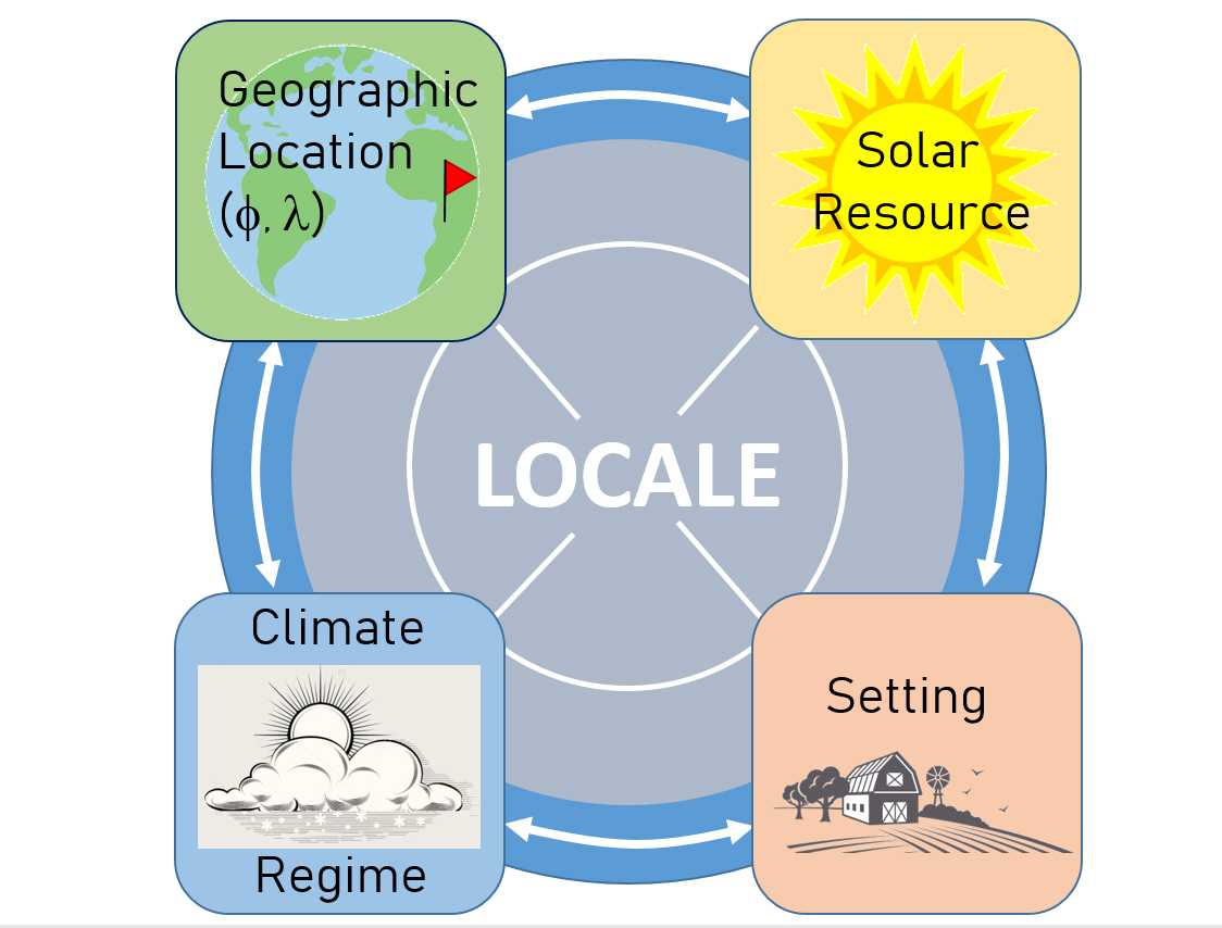
Note that locale does not refer to the design elements of the SECS (when we describe the locale, we do not yet have system in place), neither it considers client. Those two things will come into play next.
Your client (an individual, a corporation, a society?) and your stakeholders
Your "client" is a utility maximizer. They may (or may not) make rational decisions to implement a SECS. Your function in the solar design team is to be their informed advisor. However, your client may also be a whole cohort of people, or a group of stakeholders. Stakeholders are all those affected by the decision to design and install a solar energy conversion system (SECS). These may include the client, the engineers and installers, building managers, the local community members, and so on. Again, a stakeholder can be a client or just an invested individual participating in the system as a whole. One of your jobs is to identify stakeholders and asses the role their multiple perspectives may play in the design process.
Common business language states that the customer is always right. More appropriately, the customer is always the one who decides "go" or "no go" in a solar project. The basic logic of that statement guides the design process. Every SECS is designed with the needs and requirements of a client in mind. No particular system can be used by all clients in all locales regardless of how well the said system is designed. Design requires that we have a close understanding and appreciation of what a client needs. A solar designer may start the design process by posing questions to the client, such as: How much power/energy do you need? How many hours of power do you need and what time during the day do you need this power? Is this power needed year round, or only during particular seasons? Answers to these questions will ultimately guide the designer and lead to efficient design.
Your design team holds stakeholders to the concept of the Four Es: Everybody Engaging Everything Early (developed by PA design firm 7Group [147]). We want to engage the stakeholders in the integrative design process, and the pre-design process can involve brainstorming events called charrettes.
The design team also needs to educate the client on the different options available to him/her. For example, if a client decides to install photovoltaic panels to provide electricity, the design team will need to inform the client on the various PV technologies, the advantages and disadvantages of each in regard to price and function in different locales, the different options for funding the project through government grants and loans, etc.
As such, your client (and associated stakeholders) and your locale are the two major super parameters that can guide systems design.
Self-Check
6.3 Engineering Tools to Maximize Solar Utility
Reading Assignment
- J.R. Brownson, Solar Energy Conversion Systems (SECS), Chapter 6: "A Comment on Optimal Tilt" (small section at the end of the chapter) and see Figure 6.16.
Optional Reading
- M. Lave and J. Kleissl. (2011) Optimum fixed orientations and benefits of tracking for capturing solar radiation in the continental United States. Renewable Energy, 36:1145–1152.
- C. B. Christensen and G. M. Barker (2001) Effects of tilt and azimuth on annual incident solar radiation for United States locations. In Proceedings of Solar Forum 2001: Solar Energy: The Power to Choose, April 21-25 2001
- T. Huld, M. Šúri, T. Cebecauer, E. D. Dunlop (2008) Comparison of electricity yield from fixed and sun-tracking PV systems in Europe. European Commission, Joint Research CentreInstitute for Energy, Renewable Energies Unit, via E. Fermi 2749, TP 450, I-21027 Ispra (VA), Italy (poster, PDF)
- Greentech Media Article: Solar Balance-of-System: To Track or Not to Track, Part I [141] (Nov. 2012)
Engineering Approaches to Increase Solar Utility
Locale is the space or an address in time and place within which the client occupies and demands energy resources. Recall that our clients are on the demand side of solar goods and services, and as such they seek maximal utility when making decisions.
The goal of solar design is to:
- Maximize the solar utility
- for the client or group of stakeholders
- in a given locale.
We have already learned that the solar resource can be affected by the locale of the site. The solar resource is determined by the locale, as the climate regime affects the seasonal and daily irradiation patterns and frequencies of intermittence. The character or quality of the solar resource will in turn constrain the design team's options for technological solutions that compete with conventional fuel-based technologies.
According to our review of SECS Chapter 6: given that goal for solar project design, we have three main engineering approaches that we can leverage to affect the solar utility for a client in a given locale:
- Reduce the cosine projection effect on an aperture/receiver. These are the extreme angles of incidence (also called low glancing angles);
- Reduce the angle of incidence () on an aperture/receiver; and
- Reduce losses from shading on an aperture/receiver.
These are the three main engineering parameters linked to the locale that will constrain your design options (you can look back to the Angular Solar Symbols guide [43] to refresh your memory). They all affect system performance, without necessarily directly influencing the cost of the system (in the beginning). Let's review how they affect system performance.
Reduce the cosine projection effect

(). The bottom image shows the cosine projection effect as it affects the Sun-Earth view factor (the inverse cosine of the zenith angle reduces the intensity of the Sun's irradiance).
How does the tilt and azimuth each affect the design in SECS, and how does regionality affect the design decisions in solar energy?
We have seen in our reading of Lave and Kleissl that an annual optimum for tilt and azimuth can be selected, while Christensen and Barker demonstrate that annual optimum is not really "peaky," and fixed-tilt systems can be oriented across a broad range of directions in a given locale without dropping solar gains by more than 10-20%. If we were to adjust the tilt for a seasonal optimum, we would select a lower tilt for the summer season and a higher tilt for the winter season. Effectively, we are working to correct for the cosine projection effect of our particular latitude and climate regime (one climate regime per season, recall the "fingerprints").
On broad scales, sites near the equator will have different design constraints than sites near the Arctic Circle, due to the cosine projection effect driving our solar resource across latitudes and the seasons. In this context, the project locale serves as an effective system constraint. The amount of sunlight available on a daily basis and on a seasonal basis differs with locale. Using and implementing the same system design for a client in State College, Pennsylvania (, ) and another in Lagos, Nigeria (, ), for example, will yield totally different results and lead to unsatisfied clients.
You see two images of a cartoon Sun, drawn from Ch 4 of the SECS text. The top image shows the effect of inverse square law on the Sun-Earth view factor (). The distance of 150 million km reduces the intensity of the Sun from to 1361 |(). This effect is fairly uniform year-round. The bottom image shows the cosine projection effect as it affects the Sun-Earth view factor. Here, the inverse cosine of the zenith angle ( ) reduces the intensity of the Sun's irradiance. Hence, the farther away your client is located from the Equator, the more the designer will need to make collector orientation adjustments to compensate for the losses from the cosine projection effect.
Note also that the tilt of the Earth's axis will drive one to consider summer or winter optimized orientations (away from the Equator).
Reduce the angle of incidence
How does tracking affect the design decisions in solar energy?
Well, a fixed axis SECS is often oriented toward the equator at a tilt ( ) somewhat less than the local latitude (do not fall for the latitude = tilt rule of thumb), per our readings from Christensen and Barker, and Lave and Kleissl. When we track the Sun, then more beam is collected (the angle of incidence tends to be consistently lower than for a fixed tilt). By looking at the poster from Huld et al. (2008), we see that a single-axis tracking system, with an axis inclined at an optimum angle towards South, should offer 12-50% improvement over a fixed axis tilted at the optimum, where a 2-axis tracker will offer a very similar solar gain of 13-55%.
So, a tracking system will minimize the angle of incidence ( ), but there will be a cost in terms of land requirements. Why? Because of shading. There will also be a cost in terms of the balance of systems (e.g., the non-SECS trackers). This is why we could read "Solar Balance-of-Systems: To Track or Not to Track, Part I" for more information.
But the reality of solar development (whether on a rooftop or on a field) is that the systems are often "area constrained." We can make certain tradeoffs in systems choices to deliver a better unit cost to the client, but we may not get all the land that we desire to accomplish an optimal tracking system. As such, we must work with the stakeholders to find the highest solar utility solution given the available area.
Reduce losses from shading
Finally, a large group of our SECSs rely on access to the shortwave light from the Sun. If we shade a collector, then we reduce or remove that working energy that we wish to convert to heat or electricity. We performed the shading analysis in Lesson 2 using orthographic and spherical projections specifically to be able to avoid shading of our array over the course of an entire year.
Of course, if we were to design a system to avoid the Sun's rays, that would be different. We have seen examples of solar design for Parasoleil frameworks (shading systems) in the beginning of the textbook (e.g., southern awnings).
Self-Check:
6.4 Discussion Activity
Lesson 6 Discussion in Yellowdig!
In this lesson we continue making connections between the technical information on solar resource and system design with project economics.
- First, review the recommendation for the engineering principles - cosine effect, angle of incidence, shading. There are some common "rules of thumb" on how to position the panels, and there are some additional methods and tools to maintain the highest possible efficiency. Share any methods and tips you find.
- If you are developing a project in Madison, WI (43o N) or Melbourne, Australia (-37.5o S), for example, what panel position would you recommend to the client. Would you go with the fixed tilt, trackers? How would your recommendations be related to the area constraints? Suggest some scenarios here.
Then, we also collect various weather and climate information about the locale. Some supporting information is available from the TMY data, environmental monitoring stations, or direct measurements. Seasons may look different in different climate zones. How do we relate all that information to the SECS performance?
- Whats is the impact of air temperature? Why do we collect and report this information in system design justification?
- How do the data on clearness indexes (KT) help us in decision making about system design and capacity?
- What about humidity, preciptation, particle concentration - is that information important?
Those characteristics of the locale are not just FYI. We are trying to reveal their economic impact on system performance, payback, and return on investment for our client.
Tagging
We will revisit some of the previous topics in Yellowdig (maybe at somewhat different angle) and will add some new as well to provide you with the discussion space on the questions above:
You can tag your post with one or several topics at the same time (just be sure to address all those in your post). All posts and contributions you create are added up to one score at the end of the week.
Importance of interaction
Yellowdig tip: Remember to respond to questions. If your post generated some, it is a good thing! The best way not to miss questions is to set email notifications in Yellowdig - then, whenever someone reacts to your post, you will get instantly notified.
Grading and Deadline
Remember that Yellowdig point earning period ends each Friday. Posting commenting, reacting regularly through the weeek will make the 1000 pts. an easy target and guarantee a high participation grade in the course. Yellowdig discussions will account for 15% of your total grade.
6.5 The Power Grid System
Reading Assignment
- J.R. Brownson, Solar Energy Conversion Systems (SECS), Chapter 9: Solar Economics (focus on Managing the Grid)
Power Grid 101
One of the highly visible SECS technologies is photovoltaics, which delivers (generation) electricity to the client, and now pushes excess electricity onto the electricity power grid. The electricity power grid is the physical system that delivers (transmission) electricity from the place where it is generated to the site where it is used (end-use, demand).The electricity leaving the generating station enters a sub-station with a step-up transformer that raises the voltage extremely high for long-distance transmission.
When electricity travels through wires (a conductor), some energy is lost, but less energy is lost when the electricity is transmitted at a higher voltage. At a high voltage, the same amount of power can be transmitted, but using a lower current. The amount of energy lost from the conductor is called line loss, and line losses are directly proportional to the current. By reducing current, we reduce losses for the same power transmitted. Typically, in the U.S., line losses between generation and end-use are in the 6% to 8% range.
The high-voltage electricity is carried over transmission lines to local substations, where a step-down transformer reduces the voltage to levels suitable for customer loads. Distribution lines carry the lower-voltage electricity from the local substations to customer sites.
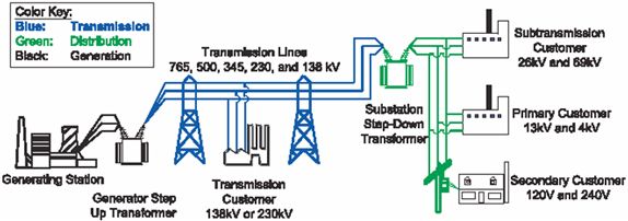
On the left, there is a Generating Station with a line going into the “Generator Step Up Transformer”. This is the Generation portion of the diagram.
From there, it goes to the Transmission Customer (138kV or 230kV) and to Transmission Lines (765, 500, 354, 230, and 138kV). This is the transmission portion of the diagram.
From the Transmission Customer and Transmission lines, it goes into a Substation Step Down Transformer for distribution. This is the Distribution portion of the diagram.
From there, it goes to the Subtransmission Customer (26kV and 69kV), the Primary Customer (13kV and 4kV), and the Secondary Customer (120V and 240 V).
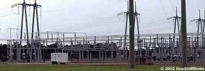
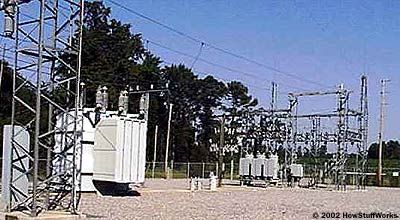
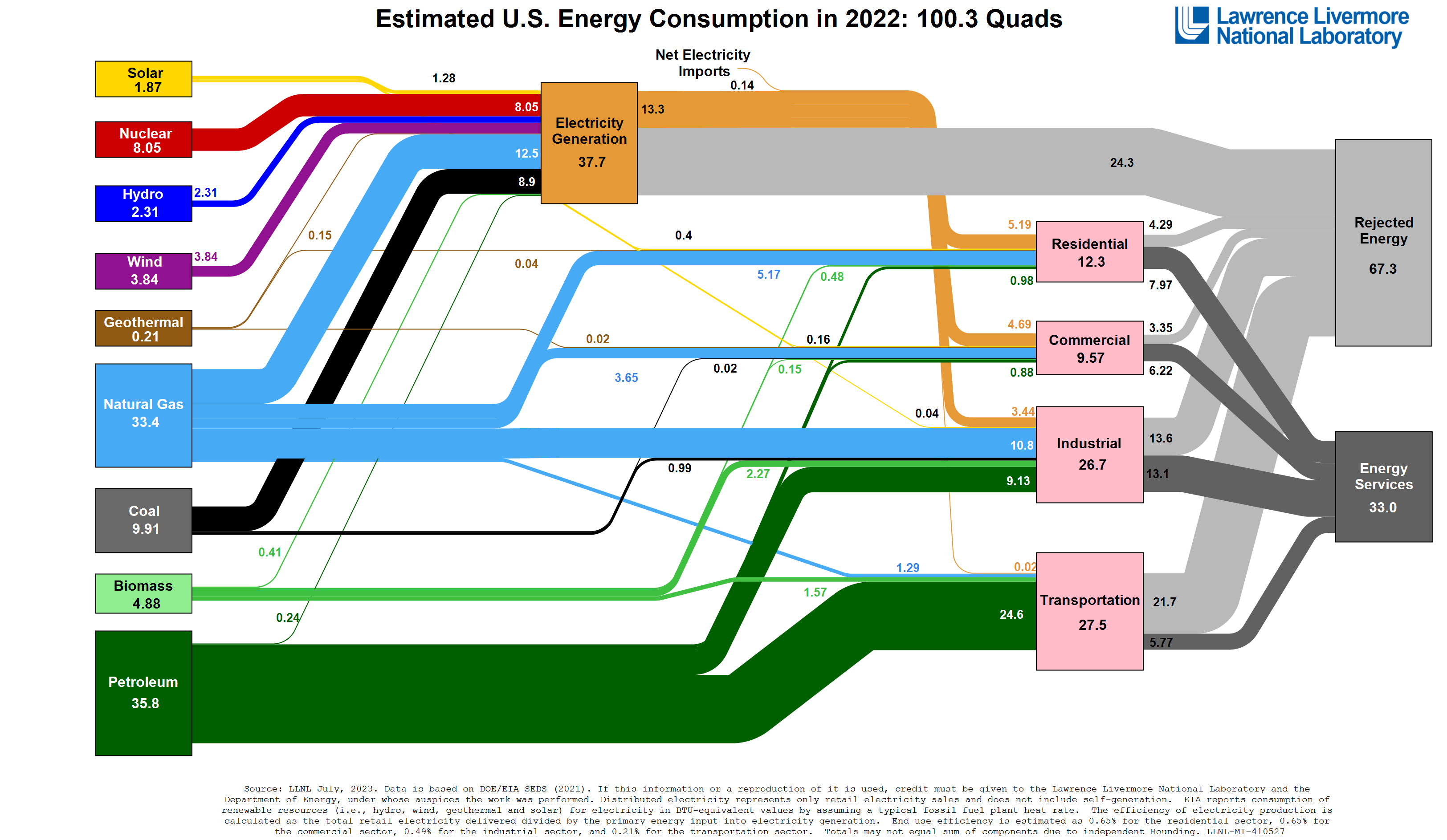
Try This!
The Power Grid [150] is a simulation created by the Cyber Resilient Energy Delivery Consortium for education.
- Access the Power Grid animation.
- Examine the "Quick-Start Guide" as a helpful resource.
- Play with the simulation to understand the relationships.
Grid Energy Storage
Primitive as it may seem, the energy storage technology that is "grid-tied" and having the largest capacity is accessed by simply pumping water up to a higher elevation, and storing it as potential energy. Called pumped storage, or pumped storage hydroelectricity, the energy is recovered when the water from the higher elevation is used to drive turbines for hydroelectric power conversion.
The Energy Storage Association [152] reports, "Pumped storage hydropower can provide energy-balancing, stability, storage capacity, and ancillary grid services such as network frequency control and reserves." While the US has 20 GW of installed capacity, worldwide over 100 GW of capacity exist. The US figure accounts for roughly 2% of the country's generating capacity, while other areas' figures are as high as 10%.
All in all, however, this process uses more electricity than it produces. So, why do it? When a power plant has extra capacity, it generates electricity used to pump water uphill. Then, when the plant is stretched to capacity and electricity is at its highest price, this pumped storage can be used to generate low-cost hydroelectricity.
Reference:
Modified from Vera Cole, Power Grid, EGEE 401 [153]. Accessed October 2013.
6.6 Power Grid Pricing and Capacity
Reading Assignment
- S. Stoft (2002), Power System Economics (pp. 30-39, 40-48; in two chunks)
- J.R. Brownson, Solar Energy Conversion Systems (SECS), Chapter 9 Solar Energy Economics (Section on "Managing the Grid")
The main form of energy that we think of in society is power from electricity. As a society, we typically deliver electric power through a complex distribution system called the power grid. In this reading, Stoft provides a fairly useful background to the pricing of utility scale electricity. I think that exposure to this content will be very helpful in your career development with solar and power systems.
As supplemental reading, you can also review the text on ISO/RTO strategies in the SECS chapter on Solar Economics (also citing Blumsack as below), and we will jump ahead briefly to Ch 14 to show a PV example of capacity factor.
Pricing Energy, Power, and Capacity
The first reading from Stoft presents the core metrics being evaluated (energy, power, and capacity) and their associated utility scale pricing units of $/MWh.
- Energy is measured in units of MWh, priced as a stock in units of $/MWh
- Power is measured in units of MW, priced as a flow, but over a block of time in $/MWh
- Capacity is measured in units of MW, also priced as a flow in $/MWh
Capacity is likely the newest term to everyone; it is a measure of the potential for power delivery. The price of power or capacity is metered as monetary units (dollars, euros, yuan, etc) per time unit of an hour, per MW of power that flows. The price of energy is just dollars per MWh (analogous to dollars per MJ), which end up as the same effective unit cost metric, but from different perspectives.
- $0.12/kWh is the same price as $120/MWh
- $0.06/kWh is equivalent to $60/MWh
In traditional power systems, we have turbine-generators that yield power from spinning magnets. A generator size is set by the maximum power production it can yield, measured in units of MW. We pose the capacity of a generator in terms of the potential to produce a flow of power in MW, the same units as power.
The capacity factor is the fraction (from 0-1; or a percentage from 0-100%) of flow utilization over the duration of a load. We find this fraction as a ratio of the power generator's true output (evaluated over a period of time, such as a month) relative to the potential power output that would occur ideally when operating full out (nameplate capacity) for an indefinite period of time.
- See the EIA's Website for capacity factor [154].
- See Wikipedia's breakdown of capacity factor [155].
The capacity factor (cf) of a fueled power plant (coal, NG, fission reactor) can have a range depending on the applied technology >>30-40%. However, the capacity factor of PV is highly dependent upon the solar resource of the locale.
- Consider that night event will automatically drop solar capacity to 50% (annually),
- then the intermittency from clouds will deliver more drops in potential,
- finally, the conversion efficiency of a PV panel will drop the capacity a bit more.
For example, the capacity factors for PV in the USA range from 10.5% in Alaska, to 18-19% in most of the USA, up to 26.3% in Arizona, Nevada, and New Mexico. [see Table 14.2 in SECS, Brownson]. The capacity factor for PV in sunny Germany is about 11%, while the cf calculated for the desert regions of Peru is >25%.
Grid Management: Markets
The second reading by Stoft links in with our prior reading of Solar Economics in SECS and the role of market supply and demand for electricity. Electricity is not easily or efficiently stored in large amounts--we don't have pumped hydro storage everywhere, and large-scale batteries are not ready for the utility market.
In an electricity grid, power generation and power consumption must be closely matched at all times. These are key concepts in our understanding of electricity. If power generation and power consumption get out of balance, blackouts and other systemic failures occur.
- Interconnection: a network of interconnected power grids within a region. The USA has three: two major interconnections in the Eastern Interconnection and the Western Interconnection, and the third is in Texas (yes, TX has its own interconnection). That is 3 separate power grids in the lower 48 states.
- Regional Transmission Operators (RTO) / Independent System Operators (ISO): not-for-profit organizations whose job is to act on behalf of a group of electric utilities in a region, managing and maintain a joint and stable power transmission grid. RTOs can establish centralized spot markets in electric power and ancillary services, and financial contracts for hedging against transmission congestion.
- Locational Marginal Prices (LMP): the RTO provides LMPs on the wholesale market through a centralized dispatch, which reflect the social cost of transmitting electric power to a specific location within the managed system.
Reference:
S. Blumsack. Measuring the benefits and costs of regional electric grid integration. Energy Law Journal, 28:147–184, 2007
6.7 Energy Portfolio Standards and Government Incentives
Reading Assignment
- J.R. Brownson, Solar Energy Conversion Systems (SECS), Chapter 9: Solar Energy Economics (Please pay particular attention to on Government and Markets).
- N. Pfund and B. Healey. (2011) What would Jefferson do? The historical role of federal subsidies in shaping America’s energy future. Technical report, DBL Investors. (PDF available on DBL Site. [156])
- Optional: DSIRE (NC Solar Center) Database of State Incentives for Renewables and Efficiency [142] (Please find your state or a favorite state, and the Federal incentives.)
In this reading, we are digging in to the lever of microeconomic incentives. To increase solar utility for a client, or to increase the preference of the client to solar goods and services, there exist incentives for solar that effectively internalize a positive externality. While you read Chapter 9 and scan the paper by Pfund and Healey (look to the summary and the key graphics at first), I want you to think about the following:
- What is the link between Energy Portfolio Standards and Solar Renewable Energy Certificates?
- What is an "externality" in a market sense?
- Have other energy resource systems been supported by government in the past?
Government Influence on the Developing Renewable Energy Industry
How Can Policy Impact Consumer Choices?
In other nations about the world, policy for renewable energy development can emerge at either a national or regional level. In the United States, there are currently no over-arching Federal mandates requiring the development of alternative energy power generation. Thirty-three states have varying standards and mandates for the production of renewable energy for power generation.
To see this diversity of strategies, we can review the Center for Climate and Energy Solutions [157] report of Renewable & Alternative Energy Portfolio Standards.
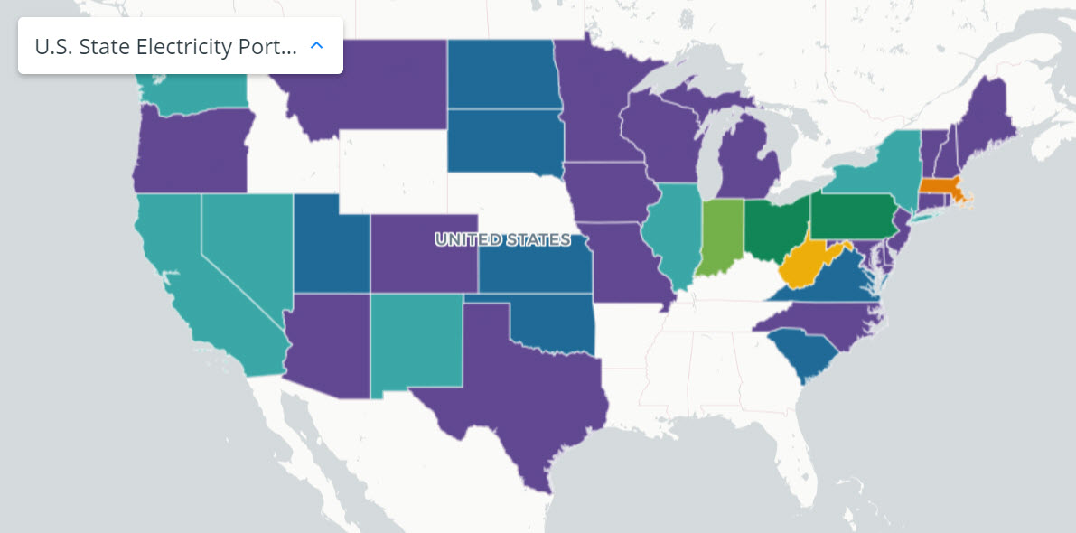 [158] [158] |
Try This! Interactive Map of US Electricity Portfolio StandardsClick on the image to access the interactive map showing the electricity portfolio standards for each state. Click on each state to see the updated renewable or alternative energy goals and milestones. |
The legislative process in various states has influenced how these programs have evolved. If we look at the states that have "alternative energy portfolio" standards rather than renewable energy portfolios (Michigan, Ohio, West Virginia, and Pennsylvania), we note that all of those states have significant industries such as auto, coal, steel, etc. One needs to consider the various reasons why these portfolios were outlined as "alternative" as opposed to "renewable." You should also develop an awareness for those states that have no standards whatsoever, and consider what impact this has on solar development. For example, we may consider that Wyoming has a very small population with the highest per capita energy demands, while being abundant in coal.
- Consider the Pennsylvania [Alternative Energy Portfolio Standard] : 18% by 2020 (with at least 0.5% carved out for PV solar)
On December 16, 2004, Governor Edward Rendell signed into law Pennsylvania's Alternative Energy Portfolio Standard, requiring that qualified power sources provide 18.5 percent of Pennsylvania’s electricity by 2020. There are two tiers of qualified sources that may be used to meet the standard.
- Tier 1 sources must make up 8 percent of the portfolio, and include wind, solar, coal mine methane, small hydropower, geothermal, and biomass. Solar sources must provide 0.5 percent of generation by 2020. However, the source of the solar power could be delivered from anywhere in the PJM ISO area, so that small fraction was depleted quickly and led to a crash in prices for SRECS (which we will talk about next).
- Tier 2 sources make up the remaining 10 percent of the portfolio, and include waste coal, demand side management, large hydropower, municipal solid waste, and coal integrated gasification combined cycle.
- You can read more about the Pennsylvania AEPS by directly reading the bill itself - AEPS. [159]
- You can also visit the Pennsylvania Public Utility Commission's site describing the program - PA AEPS site. [160]
SRECS: Market Drivers
Unique markets have been created by government stimulus of the renewable energy industry. A key market driver has been the capacity markets that have been formed in several states. In these markets, Energy Distributions Companies (EDC) are required to purchase Solar Renewable Energy Credits (SREC) or face steep fines in order to facilitate the states' requirements for renewable energy. (SREC Trade: SREC Online Auction [161])
|
States with SREC Markets |
States eligible to sell into other state SREC markets (All states eligible in NC) |
States with a Renewable Portfolio Standard solar requirement, but no SREC market yet |
Remaining States |
|---|---|---|---|
| District of Columbia (PA) Delaware (DC, PA) Maryland (DC, PA) Massachusetts New Jersey (DC, PA) North Carolina (DC, PA) Ohio (DC, PA) Pennsylvania (DC, OH) |
Illinois (DC, PA) Indiana (DC, OH) Kentucky (DC, OH) Michigan (DC, OH) New York (DC) Tennessee (DC) Virginia (DC, PA) West Virginia (DC, PA, OH) Wisconsin (DC) |
Arizona Colorado Missouri Nevada New Hampshire New Mexico Oregon Texas Washington |
Alabama Alaska California Connecticut Florida Georgia Hawaii Idaho Iowa Kansas Louisiana Maine Minnesota Mississippi Montana Nevada New Jersey North Dakota Oklahoma Rhode Island South Carolina South Dakota Utah Vermont Wyoming |
Something to look at closely is that in Massachusetts and New Jersey specifically, these credits can't be sold or purchased outside of the state. This has a significant impact on how these markets operate. New Jersey has outpaced all other states in the eastern PJM grid in the production of power from Solar PV. An unexpected development in the REC markets has been the pace at which these markets have met and exceeded the portfolio standards. Please note how this has impacted REC pricing.
Points of reference:
PJM originally stood for Pennsylvania, New Jersey, Maryland. It is simply known now as PJM; however, the grid it operates is now much larger.
PJM is the grid operator for all or part of 13 eastern states. It is the market through which Energy Distribution Companies (EDC) purchase power from Energy Generation Companies (EGC)
PJM is also responsible for charting future requirements of the grid and its users. It makes recommendations to its members, the EDCs and EGCs, regarding how to best meet these requirements. It is the principal link between the state regulated EDCs and the non-regulated EGCs. PJM is a non-profit corporation.
The Generation Attribute Tracking System (GATS) of PJM Environmental Information Services (EIS) has been instrumental in finding out trends including the growth of solar, captured methane, hydro, wind, and other renewable resources of production within PJM. The GATS has shown that based on the number of certificates generated, from 2005-2015, wind production has increased around 4,000%. In 2005, solar energy generation stood at 100 MWh, and increased to 81,000 MWh in 2009, which is a growth of 3,000%. In 2015, it stood at 2,900,000 MWh, a growth of 29,000% in a decade. Source: pjm [163] EIS [163]
In normal markets, supply and demand are the key drivers. A good deal of the growth of the renewable energy industry has been driven by regulation and government subsidy. So, conventional market drivers appear to be misaligned.
Of note is that renewable energy for the foreseeable future will continue to be an incredibly small part of power generation. What role will natural gas play in the future of our energy mix? I think it will have a significant impact on Pennsylvania because of the Marcellus Shale formation. Nuclear power could also grow at a significant rate should much smaller, localized nuclear power plants be developed that would enable cities and industrial sites to have their own sources of energy. Source: MIT Technology Review [164]
Why Incentives and Taxes? Externalities
From our reading, we have seen that there are market failures in our energy industry, both from the negative externalities of emissions (greenhouse gases, SOx and NOx, and aerosols) and from the positive externalities of using SECS technologies that provide carbon neutral energy.
In the presence of a positive externality, the social value for a good exceeds the private value. Government policies can correct this form of market failure by subsidizing the good. In the presence of a negative externality, the social cost exceeds the private cost. Policies can be implemented to correct this market failure by taxing the emissions of Pigovian tax [165]).

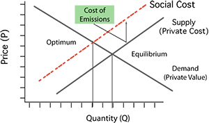
Examples of Past Government Incentives
After reading Pfund and Healey (2011), we should see that other energy sources displayed a higher social value in their own time. At the time of the late 1700s, coal was perceived in a similar fashion to our solar energy technologies like PV in the 1970s when it had several detractions, such as its bulk that made coal difficult to transport. States provided tax exemptions and incentives to move coal along, such that it surpassed timber as an energy resource in the late 1800s.
"Nature made coal abundant, policy made it cheap." p. 14
(cited from Sean Patrick Adams, The Journal of Policy History Vol. 18, No. 1, “Promotion, Competition, Captivity: The Political Economy of Coal” (2006)).
Self-Check
References:
Modified from ENGR 312, Sustainable Energy Entrepreneurship, by Wieslaw Grebski, Shaobiao Cai, and Christopher Flynn;
Penn State Hazleton. Accessed May 2013.
6.8 Electric Incentives in SAM
Try This! SAM Financing, Incentives and Utility Rate
We just talked about all these things that affect the cost of an energy system, and now let's take a look to see how the real data can fit into our simulation software for project design. Time to break out SAM again and do some exploration!
Software: SAM from NREL
The basics:
- You can open up SAM [37] at this point and click the button "Create a New File."
- Click on "Photovoltaics (Detailed)" on the left of the pop-up window ("Choose a performance model").
- Click on "Residential (Distributed)" on the right of the pop-up window ("then choose from the available financial models").
- Hit "OK."
- You will now have a default residential PV project, based in Phoenix, AZ, just like the last example we tried.
- Next, we are going to explore three tabs: Financial Parameters, Incentives, and Electricity Rates.
Financial Parameters:
- Click on the shortcut tab called "Financial Parameters."
- This opens a field of data entry for "Loan Type," "Residential Loan Parameters," "Analysis Parameters," "Tax and Insurance Rates," "Property Rates," and "Salvage Value."
The first few things to notice is that the Loan Term (and Analysis Period) is 25 years as a default. This is the standard period of covered life for a PV module. Much like your computers, the actual life will be longer than the warranty, but 25 years is the most risk that the manufacturers will currently take on to guarantee their products. In general, all the SAM defaults are going to be conservative, and you can indeed adjust them for your own projects.
You want to enclose your period of loan or mortgage ( ) within the full period of evaluation ( , years of analysis), so that . The loan rates are assumed to be a bit high, but you could change it to a lower rate if appropriate.
Tax, insurance, and property rates can be left at the defaults unless you know better from practical experience. When working with a full team in industry, you will need to be working with an expert knowledgeable in these areas to accurately represent them for the client.
The salvage value will almost never be zero in a real project. Just think, a PV system at the end of 25 years may be operating at 60-80 percent of its original peak performance, but will not catastrophically fail that year. In fact, it will likely keep on truckin' for decades more. Even a 20-year-old operational truck has a resale value that is a significant percentage of the original value. So, change it to something greater than zero, but less than 100, and you can still be conservative.
Incentives:
- Now, click on the tab for "Incentives." You can see at the top that there is a direct link for the DSIRE website [166].
- There are five types of incentives listed, each with Federal and State entries. Some also have open fields to enter utility incentives or space for an alternative incentive from another source. They also have time horizons within which the credits or incentives are valid. Check the DSIRE site for the credits and incentives in your locale!
- Investment Tax Credit [167](ITC): this is the standard federal tax credit of 30% for installed solar systems, for both residential and commercial properties.
- Production Tax Credit [168] (PTC): has been a common inscentive for wind farms, hydro, geothermal, biomass and now has been reinstated for solar generation projects under the Inflation Reduction Act (2022). This is per-kWh-generated tax credit that reduces the tax liability of solar projects. It is inacted for the first 10 years of system operation (Energy.gov [169], accessed 2023).
- Investment Based Incentive (IBI): an incentive to reduce annual expenditures of a project for Year One cash flow (see help menu in SAM).
- Capacity Based Incentive (CBI): similar to an IBI, in that it is an incentive to reduce annual expenditures of a project for Year One cash flow. However, the CBI can be expressed as a function of the system's rated capacity in Watts (see help menu in SAM). This is a direct cash incentive.
- Production Based Incentive [170] (PBI): This is another direct cash incentive, and a PBI reduces the project's annual tax liability from years one through the period of valid application (which you can specify). The PBI is a dollar amount per kilowatt-hour of annual electric output. You can use the PBI inputs for SRECs that are paid on a $/MWh basis. The PBI can also accept Performance Based Incentives [171] such as a Feed-In Tariff.
Electricity Rates:
- Now, click on the "Electricity Rates" tab. You will see whether or not "Net Metering" is occurring in your model. In most cases, this will be "Enabled" with a checkbox and a Year end sell rate (this is low, not the rate that you pay).
- The top left box is a handy link to search for electricity rates in the USA from the OpenEI utility rate repository [172]. The Open Energy Information (OpenEI) [173] provides powerful centralized access to the latest data and energy information, and an opportunity to make new tools to interpret those data and dynamic information sets.
- There is a middle hidden box (Blue plus sign) for "Description and Applicability" that is for your own record keeping, to assign the locale information for your client's site.
- You can select "Net Metering" if the locale permits electricity from a SECS to enter the grid. The Solar Energy Industry Association has a good site describing net metering in the USA [174]. Obviously, this is important to a residential or commercial PV system, but has to be adapted for a solar thermal hot water scenario (all SAM inputs are in terms of electricity).
- The electricity rates can either be "Flat" (same $/kWh charge in a month, regardless of time of day) or "Time of Use (Energy Charge)." The local electricity provider will be able to specify the selection.
- On top of electricity rates, there are charges for services, bundled as "Fixed Monthly Charges."
- Some utilities will specify "Peak Demand Charges" for high demand blocks of time (high LMP periods for the locale), and "Tiered Rates (Energy Charge)" for various scales of electric demand in kWh.
- Finally, notice that little box in the upper right called "Annual Electricity Cost Escalation". The default is for SAM to assume that the price of electricity will not go up in the next 25 years. The rate is set to zero. I will pose that this is not really an appropriate guess given our future in energy demand. A conservative increase of 1-3% is probably a better estimate.
Please Comment!
If you have any questions or comments, please post them to the Lesson 6 General Questions Forum.
6.9 Learning Activity: Pre-Design Charrette Plans
Congratulations! Your design team has been hired by Costco Wholesale Corporation [175] to propose solar integration in one of their regions (to showcase one of their commercial retail buildings in each location). Your job is to make a short written survey of the case, suggesting a plan to maximize the solar utility for their regional management in Texas.
Building Location: Austin, TX
I would suggest you develop the outline that addresses three topics that commonly occur in a solar integration discussion: (1) energy efficiency, (2) adding solar technologies on site or off-site, and (3) economic and environmental rationale.
Here is the suggested structure:
- General Information for Locale (in its diverse meaning)
- Building Energy Information: energy demand (known or approximated), energy provider, energy sources, e.g. natural gas, electric., etc.)
- Location/Site Analysis for SECS: Area available for SECS: PV / Solar Hot Water Systems / Passive solar / Solar roof control (white roof, green roof)
- Energy Efficiency Strategies: SECS efficiency considerations and building energy efficiency/conservation
- Key Stakeholders (not only Regional Managers)
- Economic Considerations
- Environmental Considerations
Resources:
- Another company previously developed a similar summary for Costco NY location. It is available to you as an example (see Canvas), but resist to just copy their format - you can do a better job organizing and presenting your data!
Diverse resources available from the USA Dept. of Energy:
- Open EI [173]: Energy Information Database
- Buildings Performance Database [177]
- Green Power Network [178]
- Database of State Incentives for Renewable Energy [166] (NCSU and DoE/NREL)
There are also extensive resources available at the 7Group website [147].
Submission:
Submit your outlines as PDF files in the Canvas Learning Activity 6.1 Dropbox: Pre-Design Summary. Appropriately cite any references used in your report.
Grading Criteria
You will be graded on your ability to develop a compelling outline that raises new questions and provides scope for the upcoming charrette. All this is based on limited information of the actual site, but extensive access to general information about the type of building and potential stakeholders. The activity assesses your knowledge of investigating the client and stakeholders and the locale when planning to maximize solar utility in the pre-design phase.
Grading Rubric
This is a 20 point assignment
- 4 pts: include at least 4 elements of locale
- 4 pt: assess the building type (commercial retail/warehouse) for on-site energy demand
- 4 pt: assess the area/site and its suitability for installing solar technologies for local energy production
- 2 pt: assess strategies for reducing energy demand
- 2 pt: include a list of at least five types of potential stakeholders for the charette
- 2 pt: list economic questions to consider
- 2 pt: list environmental questions to consider
Deadline
See the Calendar tab in Canvas for specific due dates.
6.10 Brainstorming Your Solar Proposal
Consider this activity as a slight detour in preparation for your final project proposals in this course.
While you are still on your way through the course lessons that explore solar design concepts, it is probably about time to start thinking about a potential locale and client you want to direct your efforts towards for your couse project. This final proposal will be the synthesis of your prior work, learned skills and tools in the form of a professional project SECS design, which eventually may become the basis for the real implementation scenario.
Here are some guiding points to start this off:
- List a few (2-3) geographical sites that are of potential interest to you. Consider that the solar dataset (TMY2) needs to be available for a location nearby. This will initially limit you to several hundred sites in the USA for your SAM simulations (although data from other locations can be incorporated by synthesizing a weather file in SAM).
- Take a brief look at policies in the locale or government incentives that would make a project proposal more likely in each site.
- Address whether the constraints of site location and local/regional/federal policies might guide one toward proposing a residential, commercial, or utility scale SECS (thermal or PV).
- Finally, address the following question: If you were looking for a client base (individuals or a group of investors), who is your target audience to make a "pitch" to in a future charette?
Create a post in Yellowdig with your brainstormed project ideas using the Course Project Topics tag. Be sure to check what everyone is doing and respond with comments and suggestions and answer any questions to yours.
Deadline
I would like everyone complete their topic brainstorm by the middle of Lesson 7 week (following Sunday), so you have some extra time to search and choose until then. And this is actually a mandatory activity! I need to see what everyone's plans are for the project, so if nothing is posted, I will get back to you and bug you :)
6.11 Summary and Final Tasks
Summary
This was a pretty good lesson to help us to put boundaries around our design projects. We learned that we need to identify the constraining features of our design problem. A design effort without constraints and boundaries can quickly spiral out of control, having too many possibilities to draw from. We address that challenge using the goal of solar energy design and engineering:
To maximize the solar utility for the client or group of stakeholders in a given locale.
We found that locale in this course means a broad range of factors in time and space that affect SECS design. Locale is tied to the meteorology and physical placement of the SECS, and locale is tied to the cost of fuels (here, as electricity) and incentives available to our client.
Which brings us back to our client. We do not design to make the coolest SECS (although, a really cool SECS is pretty fun to admire and brag about), we design to offer the highest solar utility to our client, as an individual, a corporation, a community, or a group of stakeholders with financial shares in the potential development. It is the client who responds to high fuel costs (seeking a solar substitute), and it is the client who responds to incentives in project proposals. We have observed that there are market and government drivers that can strongly affect the financial portion of the solar utility argument. Keep in mind also that our clients will not always behave as rational agents within the market. It is our job to learn about the locale and the client to best serve them in the design and project development arc.
Reminder - Complete all of the Lesson 6 tasks!
You have reached the end of Lesson 6! Double-check the to-do list on the Lesson 6 Learning Outcomes page to make sure you have completed all of the activities listed there before you begin Lesson 7. And get ready for Lesson 7, because it will be a bit more intensive than Lessons 5 and 6.
Lesson 7 - Solar Finance
7.0 Overview
Overview
We are now completing the last part of a three-lesson arc in economics and solar project finance. By now, you should observe significant connectivity between the past two lessons. We have discussed the economic drivers in energy systems, the basics of clients as utility maximizers, and then addressed multiple ways in which we as designers/engineers on a team can access the goal of maximizing solar utility for our clients in a given locale.
In Lesson 7, we will discuss ways to deliver useful metrics to our clients from a finance perspective. We will approach SECS through Life Cycle Cost Analysis (LCCA), dealing with concepts of financial paybacks on investment, solar savings, time value of money for long periods of evaluation, and levelized costs of energy.
7.1 Learning Outcomes
By the end of this lesson, you should be able to:
- define the time value of money;
- describe the concept of solar fraction;
- list economic figures of merit in solar project valuation;
- process simple and complicated financial spreadsheets for solar hot water projects;
- apply solar savings evaluation to the life cycle costing of small solar projects.
What is due for Lesson 7?
This lesson will take us one week to complete. Please refer to the Course Syllabus for specific time frames and due dates. Specific directions for the assignment below can be found within this lesson.
| Required Reading: |
J.R. Brownson, Solar Energy Conversion Systems (SECS), Chapter 10 - Solar Project Finance W. Short et al. (1995) Manual for the Economic Evaluation of Energy Efficiency and Renewable Energy Technologies [179]. NREL Technical Report TP-462-5173. (selected sections) |
|---|---|
| To Do: | Discussion Activity: Life Cycle Cost Analysis for Solar Hot Water - Financial Spreadsheet
Quiz Assignment (see Canvas, Module 7) Project Topic - Submit your ideas for course project to the forum. |
| Topic(s): | Time value of money and financial spreadsheets Life Cycle Costs/Savings Solar Savings Solar Fraction Levelized Cost of Energy |
Questions?
If you have any questions, please post them to the Lesson 7 General Questions and Comments Discussion Forum. I will check the forum regularly to respond. While you are in a discussion, feel free to post your own responses if you, too, are able to help out a classmate.
7.2 The Basics: Time Value of Money and Rates
Reading Assignment
- J.R. Brownson, Solar Energy Conversion Systems (SECS), Chapter 10 (Focus on the Introduction and the Time Value of Money.)
- W. Short et al. (1995) Manual for the Economic Evaluation of Energy Efficiency and Renewable Energy Technologies [180]. NREL Technical Report TP-462-5173. (Read pp. 1-22: from Introduction through Taxes, skim pp. 10-11.)
Fundamentals
We will be considering cash flows - namely, revenues - expenses or savings - costs - in a process called Life Cycle Cost Analysis (LCCA). As you have seen in the reading, cash flows can be developed for systems operations, for investment decisions, and for financing. We will be representing cash flows in a simple, discrete pattern called end-of-period cash flow, where the periodicity is 1 year, and the compounding or discounting uses an annual rate.
- Given: SECSs tend to have life-spans that are quite long, often well beyond the 25 years of the PV module warranties.
- Also given: A lot can happen financially in 30 years! The USA has had three recessions since 1988 (list of U.S. recessions) [181], and fluctuations in the rate of inflation between 2-6%.
- And finally: SECSs are still "fresh" to many consumers and will be "foreign" systems to most clients in the beginning of a project development.
- Result: energy systems that have a long horizon of life, a long financial period of evaluation to assess, and yet existing within a dynamic financial setting: increased uncertainty and risk (without better information available).
Did you see that last bit?
Clients will perceive increased uncertainty and risk without better information available. That's your job! To provide better information and transparent project evaluation, which demonstrates an understanding of both the solar resource and the financials associated with a proposed SECS. Chapter 10 of the textbook discusses how conveying the financial metrics within a project proposal is one way to provide useful information in a transparent manner.
Time Value of Money
In Life Cycle Cost Analysis, one of the important criteria is the period of analysis, or period of evaluation. The "period" conveys a time horizon for your LCCA. If we recall our microeconomic drivers affecting the elasticity of demand, we know that the time horizon is an important factor. In our case, SECS will tend to have long life-spans.
As such, we are dealing with the concept of "value" at various points in time.
- Present Value (PV, not photovoltaics this time!): specifies worth for assets like SECSs, for money, or for periodic cash flows, where the worth is in today’s dollars, provided the rate of return is specified (as "d"). The value is processed from year "n" back to "year zero" (meaning the present).
- Future Value (FV): specifies the worth of things as a dollar value in the future. We use FV for Fuel Costs (FC) and Fuel Savings (FS) in LCCA. Costs are represented as "C" and Savings as "S." The rate of inflation is specified here as "i."
- Present Worth in year n (PWn): This is the ratio of the future costs with respect to the discount rate over time.
You will notice that the same topics are discussed in detail in the assigned reading of the Manual for Economic Evaluation by Short et al. (1995).
Discount Rates
There are two ways to represent discount rates, and you will observe both in the SAM simulation software or similar financial analysis tools. Using these rates, we can produce a discounted cash flow model (DFM) to compare projects.
- Real Discount Rate ($d_r$) indicates the actual return received by lender or investor on the project (excluding the effect of inflation).
- Nominal Discount Rate ($d_n$) refers to the total of the Real Discount Rate plus projected rate of inflation.
- Note: As such, Real Discount Rate is usually a lower value than the Nominal Discount Rate due to inflation.
- Caveat: If the inflation rate is negative (deflation) then the Real Discount Rate would actually be higher than the Nominal Rate.
The Short et al. article shows the Nominal Discount Rate loosely approximated as. But will the fuel inflation rates be the same as labor inflation rates? Or insurance inflation rates? We will have an example in the discussion where we pull apart different inflation rates and use real discount rates in the analysis of a solar hot water system.
Taxes and Depreciation
We have already seen that the DSIRE website [166] for the states and federal government of the USA is a useful resource for incentives. Part of those incentives are tied in to tax credits, and there is a significant portion of your reading devoted to the concept of depreciation.
- Depreciation: the use of income tax deductions to recover the costs of property used in trade/business or for the production of income. Depreciation does not include land.
- MACRS: Modified Accelerated Cost Recovery System [182]. You should observe that the Wikipedia site and you're reading from Short et al. will be quite similar. MACRS is used in the SAM simulation software.
Net Salvage Value
One of the things that occurs in an LCCA at the end of the Period of Analysis is the question of how to finish the summation. This is like the Monty Python movie, The Holy Grail [183], where the old fellow says: "I'm not dead!" At the end of your 15-25 year evaluation for LCCA, you will no doubt still have a fully functional SECS! They don't just break down and fall apart, and in fact they will likely last for decades beyond your evaluation period. So how do we assess the value of the system at the end of the period?
We assume that the system has a net salvage value (a resale value) that is a fraction of its initial value, translated into present dollars. In our discussion, we will assume a 20-year-old solar hot water system still has 30% of its initial value, framed in present dollars for year 20.
In this case, if the total system cost is $16,000, its 30% salvage value will be 4,800.
Applying the Present Value formula (see above), with the market discount rate of 8%, we can find:
Salvage value = $4,800 / (1 + 0.08)20 = $1,030
This will be monetary value of the system at the end of its 20-year service life.
7.3 Solar Savings and Avoided Fuel Costs
Reading Assignment
- J.R. Brownson, Solar Energy Conversion Systems (SECS), Chapter 10 (focus on Solar Savings)
Solar Savings
When I think about a SECS and the potential solar utility for a client in a given locale, I am familiar with the variable costs (VC) of fuel in a home or a commercial building. I am also familiar that SECSs have a relatively high fixed cost (FC) of the system's initial investment. So, I need a metric that can show me the annualized and cumulative flow of cash as costs and savings (in today's dollars) over the period of analysis.
We see in our reading that earlier solar engineers had developed strategic ways to apply the concepts of Life Cycle Costing Analysis (LCCA) for SECSs. Because solar technologies like PV (photovoltaics) and SHW (solar hot water) tend to substitute for fuels that need to be purchased, the authors recognized a value in specifying SECS financial potential in terms of avoided fuel costs (another FC), otherwise termed fuel savings (FS). The opposite of a "cost" is a "savings" in marginal analysis, right? But saving fuel is only one of at least seven parameters affecting the flows of cash for a system. Annualized cash flows are the sum of costs and savings in a year.
- The Solar Savings (SS) are the sum of avoided fuel costs (fuel savings) and incremental costs of operation for the SECS that we calculate for a system, typically on an annual basis, then put in today's dollars, and finally summed for a cumulative solar savings. Notice that (in the best scenarios) there are three savings parameters (+) and four cost parameters (-) assessed. Can you describe what each of these parameters is, and how they each function?
SS = FS - incremental mortgage/loan payment
- incremental maintenance/insurance
- incremental parasitic energy costs
- incremental property taxes
+ tax credit incentives
+ production credit incentives
- The Life Cycle Savings (LCS) are the cumulative solar savings for the period of analysis, framed in today's dollars.
Self-Check:
7.4 Solar Fractions: Gains and Loads
Reading Assignment
- J.R. Brownson, Solar Energy Conversion Systems (SECS), Chapter 10 (focus on the Solar Fraction and Gains, Loads, Losses)
Loads, Costs, and Fractions
We know that a local SECS like a Solar Hot Water system will have a certain quantity of demand from a residential family.
- Annual Loads (L) Example: In the Midwest of the USA, a residential family will consume 1.5-2 MWh of energy to heat water per year. That's an energetic load.
- Annual Costs (C) Example: In the USA, an average retail electricity cost is \$0.08/kWh, or \$80/MWh.
- Annual Solar Fraction (F): The fraction of energy provided by a SECS relative to the total energy demanded for the periodic step size (here, annual). In the solar field, we call the supplemental energy required beyond the SECS: "auxiliary" energy (even if it is a primary energy source in society).
We often design a domestic solar hot water (DSHW) system to provide an annual fraction F = 0.4-0.7 (40-70% of the total annual demand), sized for the summer loads, because the heat would be wasted/dumped in the summer. That would mean the client would be buying a bigger system that does not have utility in the summer. Better to have a less sufficient system for hot water in the winter, than for the client to pay for something they cannot use part of the year.
In our reading, we made the distinction between the annual solar fraction (uppercase F) and the monthly solar fraction (lowercase f). We can use the solar fraction as a factor in project finance to estimate an ideal array size for our client in his/her locale. Consider that a large solar fraction will entail more modules or panels, and will increase the cost for the client in the system investment (according to the unit cost). It will also increase the time to payback the investment. Our clients will no doubt have finite cash on hand to put a down payment into a SECS, and to acquire a loan for the rest of the investment. They may also require a fast payback that will influence the sizing of the system.
- An annual solar fraction of zero (F=0) is where the client opts for no installation of a new SECS.
- will have the highest energy costs (fuel costs; ) of any alternative SECS
- An annual solar fraction of one is where the client opts for a SECS that covers all energy loads for the entire year.
- will have the highest solar investment costs (), with the lowest associated annual energy costs
- We are to work with the client to find a strong solution between those two trivial extremes (a maximum return on investment), specifically a return with net positive in cumulative solar savings (Life Cycle Savings: LCS).
annual fuel savings (considered before discounting or fuel inflation rates)
7.5 Yellowdig Discussion
Domestic Solar Hot Water Financial Analysis
We have covered methods to account for the costs and savings for a generic SECS in the previous pages. In those readings, we introduced the time value of money. So, let's think about the "time value of money" using a spreadsheet. The questions below are to be leading topics that will dig into the coupled meanings of Life Cycle Savings, Solar Savings, Fuel Savings, time value of money, systems payback, and paying back a loan. Some of the questions may be easier than others, but there are not necessarily clear answers to all of them. Also some people in class may have more experience with this type of analysis than others, so it would be beneficial to work together as a group through this discussion.
An example spreadsheet for solar hot water systems in a residential home (Domestic Solar Hot Water, or DSHW) is published as a shared Google spreadsheet. The direct link to access the file is in the middle of this page. This spreadsheet is set up in many columns: each column is representing a separate sequence of years for discrete financial analysis. There are accompanying graphs to link with the data, presenting loan payments and annualized Solar Savings increasing each year. Because the spreadsheet is dynamic, it would be better if you download a copy of the file and try changing things like the discount rate, fuel cost, loan size, and systems size (solar fraction) and see what the response will be.
There are two example systems analyzed in the spreadsheet. The first system has a solar fraction F = 0.65, costing \$16k with a 20% Down Payment and the remainder paid through a back loan at 7% interest. The second system has a solar fraction F = 0.85, costing \$26k with a 20% Down Payment, and the remainder paid through a back loan. Both systems have a potential resale value of 30% of initial investment ($16k), framed in Present Value (a different kind of "PV"). This is a detailed spreadsheet presenting you with an example of discrete financial analysis where we consider the time value of money over 20-year span. Half the battle in developing a useful spreadsheet is figuring out where everything is. Later, we will also dig into the financial output in SAM simulations.
NOTE: You must be logged into Google in order to view this spreadsheet.
Link to Google spreadsheet [184]
Study the spreadsheet and then discuss the following questions in the Yellowdig community.
- Why is there Time "Zero?" What years do the two systems "pay back?" Why is there an additional financial increase for Year 20 at the end?
- Look at columns through and identify the role that each of the columns serves leading up to Solar Savings and the Cumulative Solar Savings (framed in present worth).
- Where does one find the market discount rates to estimate present values (seen in Column and of the first sheet), and why is it that we need to consider future values in present worth when we are accounting for the project finance of SECS? What would the special meaning of the rate be if we raised that value from 8% in Column , to a value high enough to drive the LCS to \$0?
- In the red colored "loan" columns, do you see the connection to the reading regarding the rate of the loan and the annual loan payments? Why is the interest rate listed as a "discount rate"?
- Which system would seem to be a reasonable investment for a middle-class family of 4 (two incomes, <\$100k annual gross income) living in Michigan, USA? Why?
- A comment: Columns , , and are tied to the use of fuel to heat water (annual loads: ), the annual Solar Fraction for the installed system (annual solar fraction: ), and the annual cost of the fuel ( as electricity in \$/MWh, or \$0.8/kWh). We are initially guessing a system size, and that 65% of the annual energy will be covered by this array. In mid-continental USA, each person consumes ~8 MWh of energy to heat water per year. Here, we are estimating for a residential family of four.
Deadline
There is no hard deadline for this discussion activity, but it would be good to have some initial relfections posted in the middle of the study week (Sunday), and comments and replies will be due by the end of the point-earning period.
7.6 Economic Figures of Merit
Reading Assignment
- J.R. Brownson, Solar Energy Conversion Systems (SECS), Chapter 10 (focus on the Discrete Analysis and Gotta Payback)
- W. Short et al. (1995) Manual for the Economic Evaluation of Energy Efficiency and Renewable Energy Technologies [180]. NREL Technical Report TP-462-5173. (read pp. 35-58: from Selection Criteria Guide to Economic Measures, and through Discounted Payback Period)
I want you to think about the ways that figures of merit serve as various economic metrics to allow a client to compare alternatives in energy systems selection and design in an "apples to apples" fashion, despite the fact that SECS are coupled to an intermittent solar resource. You may find it easier to read chapter 4 of Short et al., and then jump back to chapter 3 of Short et al. We will focus on the figure of merit below; but really, these pages are chock-full of useful information for future project development!
Figures of Merit
What are the figures of merit to which our clients will respond?
- Net Present Value (NPV): in our case, deals with annualized costs and revenues that account for discount rates.
- Total Life-Cycle Cost (TLCC): used to assess marginal costs and the timing of costs when comparing alternative projects. Provides no frame of reference for acceptable/unacceptable costs, and doesn't address returns and benefits.
- Levelized Cost of Energy (LCOE): used to compare alternative technologies that often have different operational periods, different scales of operation and investment, or both. The common example is comparing a renewable technology like wind or solar electricity to a generation unit that requires geofuels. LCOE is often used to rank alternatives for effective budgeting of expenditures. As different investment sizes are not considered in a unit cost, LCOE is not recommended when choosing among systems that are "mutually exclusive." The LCOE represents the costs of the system throughout its lifetime spread evenly over the energy produced by the system, It is computed as the TLCC (discounted to the base year) divided by the lifetime energy production.
- Internal Rate of Return (IRR): the discount rate at which the NPV for the period of analysis is zero.
- Discounted Payback Period (DPB): contrasted with a simple payback, the discounted payback helps to compare risk between project options.
Try This! Levelized Cost of Energy
Now that we've entertained the idea of a Levelized Cost of Energy, let's try out a web tool designed by NREL to estimate LCOE (link directs to the documentation site first). [185]
- How does "capacity factor" affect the LCOE in a renewable system, and what is the capacity factor in places like MI, MO, or AZ? If you don't know what that is, search for it in the SECS text book (I've included a table for each US state).
- What are the capital costs (range) for Solar PV? Why do you think it is a big spread?
The OpenEI (Open Energy Information; site home here [186]) has a supplemental resource called the Transparent Cost Database [187]. (Make sure you are looking at "Generation.").
- Why do you think there is such a large spread in the LCOE of solar PV and not for Natural Gas?
- Is there any weakness with using LCOE to compare power generation in a residential PV installation with the LCOE for a coal fired power generation plant?
Send Feedback!
I would value hearing back from you as to whether these tools are useful, or not so much. Please take a moment to post your perspective on whether these government-based online tools seem useful to you for the future on the General Forum for Lesson 7.
7.8 Summary and Final Tasks
Summary
Good progress, class! We have now completed our three-lesson arc through Lesson 5: economic analysis, Lesson 6: solar utility for the client and locale, and finally Lesson 7: financial life cycle cost analysis.
In Lesson 7, we read about and discussed ways to deliver metrics to our clients that would be useful for financial assessment and project comparison. We called the overall process Life Cycle Cost Analysis (LCCA), dealing with concepts of financial paybacks on investment, solar savings, time value of money for long periods of evaluation, and levelized costs of energy. We introduced solar-specific terms such as the annual Solar Fraction (F), the Solar Savings (SS), and the Life Cycle Savings (LCS).
We discovered that financial analysis can be as direct as using a spreadsheet and some basic assumptions to assess financial cash flows and energy flows, or it can be a detailed simulation using meteorological data. We used discrete annualized methods of analysis common to project management in industry.
Coming up in the next three lessons, we will add to that strategy, and you will keep developing your arguments by building from sources found on the web (or from clients).
Design is pattern with a purpose.
Whereas art and science provide mechanisms to ultimately open windows into apparent patterns about us, design and engineering are purposeful approaches to establish systems that fit the revealed pattern. [Brownson, SECS, Ch. 16]
Reminder - Complete all of the Lesson 7 tasks!
You have reached the end of Lesson 7! Double-check the to-do list on the Lesson 7 Learning Outcomes page to make sure you have completed all of the activities listed there before you begin Lesson 8.
Lesson 8 - Methods of Prediction
8.0 Overview
Overview
We encounter two really big factors that create a spread of possible outcomes for energy systems when we look into the future: weather, and people demanding energy. In Lesson 8, we will advance our knowledge regarding the role of weather and the electric power grid. We will cover a general idea of risk and uncertainty. Then, we will show again that time and space are related using Taylor's Hypothesis. More important, we will describe how events in the future can be predicted (to certain degrees of confidence) from historical knowledge and from knowledge of present events that are connected spatially to the locale of interest. In particular, we are interested in tools used by meteorologists.
Both weather systems and demand on the grid (called loads) will be presented as dynamic, coupled parameters. Both weather and grid loads will deeply affect our clients in terms of the required decisions for solar technology deployment and management. Both will be shown to have a spread of possible outcomes for a given time horizon; and thus, there will be uncertainty and risk in making decisions.
Now, the point of Lesson 8 is to familiarize yourself with modern elements of time horizons that affect project risk assessment and management due to the dynamic behaviors of the grid and of the local weather systems. We are not going to give you the full chops of a meteorologist, no more than in the last lesson were we going to turn you into a financial analyst. The whole point of transdisciplinary research and practice is for experts from different disciplines to work jointly as a team around a shared goal (e.g., the goal of solar design) to address a common challenge. However, it is hard to work jointly on a team when you don't know the language of your team members. So, onward!
8.1 Learning Outcomes
By the end of this lesson, you should be able to:
- describe the role of risk and uncertainty in delivering solar resource units to the grid;
- describe the time-space relationship in meteorological assessment;
- list the current limitations of solar resource forecasting in time and space scales;
- list the relevant meteorological metrics for common SECS technologies.
What is due for Lesson 8?
This lesson will take us one week to complete. Please refer to the Course Syllabus for specific time frames and due dates. Specific directions for the assignment below can be found within this lesson.
| Required Reading: |
J.R. Brownson, Solar Energy Conversion Systems (SECS), Chapters 5, 8, and 9 (sections related to Risk, Time-Space, and Meteorology) W. Short et al. (1995) Manual for the Economic Evaluation of Energy Efficiency and Renewable Energy Technologies [180]. NREL Technical Report TP-462-5173. (read pp. 27-34: Uncertainty and Risk) |
|---|---|
| Optional Reading (not required): | J. Rayl, G. S. Young, and J. R. S. Brownson. Irradiance co-spectrum analysis: Tools for decision support and technological planning. Solar Energy, 2013. doi: http://dx.doi.org/10.1016/j.solener.2013.02.029 [191]. A. C. McMahan, C. N. Grover, and F. E. Vignola. "Evaluation of Resource Risk in Solar-Project Financing", Kleissl, J. ed. Ch 4 in: Solar Energy Forecasting and Resource Assessment (2013) Academic Press. F. E. Vignola, A. C. McMahan, and C. N. Grover. "Bankable Solar-Radiation Datasets", Kleissl, J. ed. Ch 5 in: Solar Energy Forecasting and Resource Assessment (2013) Academic Press. |
| To Do: |
Yellowdig Discussion: Space and time relationships in solar forecasting Engage in all Try-This and Self-check activities (not graded). |
| Topic(s): | Time Horizons Nowcasting Load Forecasting Numerical Weather Prediction (NWP) Weather Research & Forecasting (WRF) |
Questions?
If you have any questions, please post them to the Lesson 8 General Questions and Comments Discussion Forum. I will check the forum regularly to respond. While you are in a discussion, feel free to post your own responses if you, too, are able to help out a classmate.
8.2 Transdisciplinary What?
You don't have to know everything...
...but you'd better have a transdisciplinary team to really be competitive in the solar market. In this lesson and the next three, we are going to explore content for which you are not necessarily expected to be the expert. But you do need to know about the important roles of your future partners in design, and the core communication topics relevant to engaging them in the integrative design process.
On your dream team for solar design, do you have a meteorologist, an economist skilled in energy business and finance, a systems engineer, a quantitative analyst [192] to assess large data, a communications expert, and a practical electrician/roofer/plumber? Yes? Well, then you're way ahead of most everyone else. OK, does your team share a common framework: such as the goal of solar design? Do they understand and work to synthesize concepts across disciplines? Do they work together to address your problems?
This is just a quick review of the term "transdisciplinary." In exploring a spectrum of techniques for the last three content lessons, we are going further and further from "core" disciplinary topics. You know, we've been saying that this integrative design process is pretty important, and it involves a transdisciplinary approach. But what does that mean, and how is it practical to the core philosophy of a solar design team?
Levels of Integrative Design Teams
- (Level Three) Transdisciplinary: contributors are from different disciplines, working jointly to explore and apply a shared conceptual framework that synthesizes discipline-specific theories, concepts, and approaches. Transdisciplinary work extends methods and concepts to address common problems, often in transformative new ways.
- (Level Two) Interdisciplinary: contributors work jointly, but still carry discipline-specific perspectives while working to address a common problem. Results tend to be reported as partial contributions in a discipline-by-discipline sequence, and each contribution of knowledge is partitioned from other relevant elements.
- (Level One) Multidisciplinary: contributors are from different disciplines, working sequentially from their own discipline-specific perspectives. The goal is to combine results at the end of the project to address a common problem.
- (Silos) Single Discipline: contributors work together within a single discipline to address a problem.
Reference:
Patricia L. Rosenfield (1992) The potential of transdisciplinary research for sustaining and extending linkages between the health and social sciences, Social Science & Medicine, 35(11) 1343-1357. DOI: http://dx.doi.org/10.1016/0277-9536(92)90038-R [193]
If we really want to see solar energy grow in new directions and adapt quickly to the diversity of challenges in society and the environment, then we need to get comfortable with "not knowing" everything, or even not knowing a lot. The patterns are generally just too big for a single person to be able to hold all of the core knowledge and be able to execute the design-build-operate process alone. We also need to get comfortable with building knowledge across disciplines, linked by a common conceptual framework. We need integrative design teams that "get" the value of transdisciplinary work.
8.3 Uncertainty and Risk
Reading Assignment
- J.R. Brownson, Solar Energy Conversion Systems (SECS), Chapter 9 (section on Utility, Risk, and Return)
- W. Short et al. (1995) Manual for the Economic Evaluation of Energy Efficiency and Renewable Energy Technologies [180]. NREL Technical Report TP-462-5173. (Read pp. 27-34: Uncertainty and Risk.)
What is Risk?
In solar project design and project management, we would like to work for our clients to minimize risk. We describe risk as the dispersion of outcomes around an expected value. Something is riskier if the spread of possible outcomes is bigger around an expected value. The more specific terms of variance and standard deviation describe the spread of data (the dispersion) about an expected value. Events that occur in the future will have a spread of possible outcomes, because we cannot know the final value for the future with 100% confidence until it actually occurs.
When we really know what to expect, what we imply is that the dispersion of possible outcomes is clustered tightly about that expectation. From that information, we can adapt or make changes for the future appropriately. However, knowing the spread of possible outcomes about an expected value is deeply important, even if you know that the spread of outcomes is very broad. The greater the dispersion of outcomes, the higher the risk. In our reading, we comment that “riskier” scenarios in solar project development, or systems operation and management, will have a larger dispersion of outcomes around the expected value.
Risk is often framed as the probability of an uncertain event occurring in the future multiplied by the expected loss should the event occur. We call the model of the probability distribution the pdf, or the probability distribution function. Note that there are specific applications for continuous or discrete distributions (cf. probability density function [194], and probability mass function [195]). If we know the probability distribution [196] of all possible outcomes, then we also know the expected value of the outcome, surrounded by the dispersion of outcomes around that expected value. If the pdf is normalized, then the probability of any event can be evaluated by integrating a section under the curve. If we integrate under the entirety of a normalized pdf, then we are integrating across all possible outcomes. The total probability is then equal to 1.
Variance in Data
A common measure for the spread of data can be the variance [197] ( ). Given a sample of multiple events, the variance is a measure of the spread of the data about an expected value or outcome. We have also discovered in our reading that a portfolio of renewable energy can potentially be used to reduce the variance of the power generation coupled to the same grid. This is something to bear in mind in the future of large, distributed PV.
In Figure 8.1, below, we present a normal probability distribution function (also called a Gaussian). Now, many distributions in solar energy are not normally distributed, but this is a starting point. The data tends to be strongly skewed toward clear days (more clear days than overcast), or bimodal in nature. Quantitative analytics often use available statistical software such as R (The R Project for Statistical Computing) [198] to estimate density functions based on discrete real data (e.g. a histogram). This is called density estimation [199]. The peak(s) in a pdf represent the highest likelihood of expected values.

Self-Check
8.4 Exceedance Probabilities: P50, P75, P90
Reading Assignment
- A. Dobos, P. Gilman, M. Kasberg (2012) "P50/P90 Analysis for Solar Energy Systems Using the System Advisor Model." [188] Presented at the 2012 World Renewable Energy Forum Denver, Colorado May 13-17, 2012.
- Rhino Energy web page: "Exceedance Probabilities [189]." Accessed Oct. 20, 2013.
Using Exceedance Probabilities
Because the solar resource is intermittent (variable), so too is the power production from a technology such as PV. The expected values and the spread for natural data like the weather is not necessarily "normally distributed" or even unimodal (one peak). This is why we often plot histograms of the data to observe the manner in which the data is spread out.
We would like to describe our level of confidence that a certain level of power production (or capacity) will be met, in order to minimize the risk in managing a system. In our "Try This" example, we saw how a data set can be summarized using quartiles (minimum, 25%, 50% or mean, 75%, and maximum). So, in this case, we would like to break the spread of data into bins that are both useful and tied to probabilities.
A value of "P50" or "P90" (or any value from 0-100) describes an annual value of power production from the intermittent resource with a probability of 50% or 90%, respectively. In fact, that quartile summary can be viewed as P25, P50, and P75. For P50, there is a 50% chance that the mean power production will not be reached at any given time. For P90, there is a 10% chance that the P90 level will not be reached.
Banks and investment firms working on wind farm projects often require P50 and P90 values of the wind resource at a location to determine the risk associated with a project’s ability to service its debt obligations and other operating costs.
-Dobos, Gilmanjavascript:submit_mid('sp_ig_all'), Kasberg (2012)
Inside of the SAM software, there is an advanced feature to evaluate P50/P90. There is an accessible database (*.cbwfdb file format, a proprietary format developed for SAM's P50/P90 capability) from the National Climatic Data Center [202] (NCDC). The database is quite large (1.1 GB) but allows us to explore a number of cases for this course.
The long term NCDC/NSRDB dataset includes the impact of large volcanic activity and other phenomena that occur on timescales larger than one year. In particular relevance to solar plants, the eruption of Mt. Pinatubo introduced large quantities of aerosols into the atmosphere that reduced incident irradiance levels between 1991 and 1993. Other variations include the cyclic El Niño and La Niña phenomena, as well as the 11 and 22 year sun spot cycles.
-Dobos, Gilman, Kasberg (2012)
8.5 Coordination Challenges in Time and Space
Reading Assignment
- Alexandra von Meier (2011) "Integration of Renewable Generation in California: Coordination Challenges in Time and Space [203]" (white paper for California Institute for Energy and Environment (CIEE))
- [Review] SECS, Chapter 5 - Meteorology: the Many Facets of the Sky (sections:"Spatio-Temporal Uncertainty" and "Robot Monkey does Space-Time")
- [Review] SECS, Chapter 8 - Measure and Estimation of the Sun (sections: "Pyranometer: Global Irradiance Measurements," "Diffuse and Direct Normal Measures", and "Satellite Measures of Irradiation")
- Optional: J. Rayl, G. S. Young, and J. R. S. Brownson. Irradiance co-spectrum analysis: Tools for decision support and technological planning. Solar Energy, 2013. doi: http://dx.doi.org/10.1016/j.solener.2013.02.029 [191].
The Grid: it's complicated
Ok, so after digging into Dr. von Meier's paper on the grid, we should have noticed a few things. First, renewables in CA are continuing to grow as a contributing portion of electricity generation. Second, the power grid linked with CA (the Western Interconnection) will have to accommodate the new sources of power just as the grid has to accommodate new loads (sources of demand). Before renewables, we had baseload power mainly from coal, nuclear, and hydroelectric, and everything was pretty smooth on the generation side of the equation. But now, wind and solar power are pushing in with "intermittent power."
In essence, renewable and distributed resources introduce spatial and temporal constraints on resource availability: we cannot always have the resources where we want them, when we want them.
-A. von Meier (2011)
This is a really neat paper, in that it points out the orders of magnitude of challenges that the markets and grid operators have to deal with on a regular basis, both spatially and temporally! And yes, you might also note that those scales were incorporated into Figure 5.10 of the SECS textbook for the Fujita relation of meteorological phenomena in space and time. You can compare the units in the von Meier paper with the table and graphic below.
We just learned that large portions of the electricity grid can be managed by an Independent System Operator (ISO, or RTO), where demand on the grid is managed through markets. That is great, but the grid also has problems that accumulate anyway, which need to be dynamically adapted to by the utilities or the clients. In our main reading, we see all the different systems elements that need to be coordinated in our power grids. These are amazingly complicated systems that are then perturbed by pesky things like weather.
Coordination in Time:
- Power Systems Management and Markets: Regulatory and technological parameters occur over time spans from years to days, to less than 1 minute (>6 orders of temporal magnitude). Pay special attention to Day Ahead Scheduling and Hour Ahead Scheduling while reading about markets.
| Temporal Phenomenon | Short | Long | Unit |
|---|---|---|---|
| demand response | 4 | 4600 | sec |
| hour-ahead scheduling | 1.75 | 7 | hour |
| service restoration | 0.5 | 28 | hour |
| day-ahead scheduling | 18.5 | 48 | hour |
| T&D Planning | 1 | 16 | year |
| Carbon emissions goals | 13 | 80 | year |
Coordination in Space:
- Regional Power Grid Behaviors: Power responses, natural stability problems within the grid, transmission congestion, and regulatory scopes can happen over distances from thousands of kilometers down to tens of meters (>5 orders of spatial magnitude).
| Spatial Phenomenon | Short | Long | Unit |
|---|---|---|---|
| DG interconnection criteria | 50 | 20,000 | m |
| voltage regulation | 0.5 | 10 | km |
| distribution feeder | 2 | 25 | km |
| transmission congestion | 25 | 1,000 | km |
| stability problems | 500 | 3,000 | km |
| CAISO | 450 | 800 | km |
| WECC | 1,600 | 3,000 | km |
The Weather: yep, complicated too...
The weather systems that we deal with have their own orders of magnitude in time and space. Let's compare the time and space for weather phenomena in the following graphic. We saw this image in Lesson 3; but now, we can see that those time and space scales above actually fit with the scales right here, described by Ted Fujita. Notice the line that trends through the data of clouds (which are the nemeses of solar energy...). From a fit of $17\ m/s$, we have a quick conversion tool to flip between characteristic time scales and characteristic distance scales! Just remember $17\ m/s$ as the FRYB relation (Fujita-Rayl-Young-Brownson), and how to convert time from hours to seconds (3600 seconds in an hour), or kilometers to meters (you don't need that conversion, do you?).
8.6 Putting it together: Supergraphic
Overlaying the Grid with the Weather
Now that we know a few things about the scales of time and space for the power grid (using CAISO and WECC for scale), we can compare it with the weather scales. Look to the top and right for the von Meier scales, and the core diagram in the center for the Fujita scales. The diagram on the lower portion shows us a rough sketch of the power spectral density for the meteorological spans of synoptic, mesoscale, and microscale weather.
By applying the average meteorological advection speed of , (which we are calling the FRYB relation for the class), we can convert an example spatial scales of variability associated with transmission congestion (red vertical bar on the right) from distances of 25-1000 km into a time horizon. The relevant time scales for meteorological phenomena exist within 25 minutes to 16 hours (involving events from cumulus, cumulonimbus, and cumulonimbus clusters interfering with the Sun's irradiation).
Alternately, we observe that the harmonic effects propagating within the grid along distances of 30-300 meters would be relevant for meteorological phenomena spanning 1.8-18 seconds. This scale of events is too small to be incorporated into the presented meteorological phenomena.
 [204]
[204]
8.7 Discussion Activity
Relations in Time and Space
You have been reading about the relations between time and space, and you have read about different time horizons of interest to the solar energy and electric grid fields. Now, let us apply that knowledge to Table 8.2 from the Chapter by Coimbra, Kleissl, and Marquez (2013).
| Technique | Sampling Rate | Spatial Resolution | Spatial Extent | Suitable Forecast Horizon | Application |
|---|---|---|---|---|---|
| Persistence | High | 1 point | 1 point | Minutes | Baseline |
| Sky-Imagery | 30 sec | 10-100 m | 2-5 m radius | Tens of minutes | Short-term ramps, regulation |
| GOES Satellite Data | 15 min | 1000 m | U.S.A. | 5 hours | Load following |
| NAM weather model | 3600 sec | 12 km | U.S.A. | 10 days | Unit commitment |
Questions to discuss:
- Based on the FRYB (Fujita-Rayl-Young-Brownson) relation of 17 m/s and the given "Sampling Rate" for each method (in Table 8.3), what is the characteristic meteorological distance scale being sampled (easy conversion)? How do those distances compare to the "Spatial Resolution" scales provided in the table?
- Now take a moment to read up on the Nyquist-Shannon Sampling Theorem [205], where you will focus on the Nyquist rate. Do all of the systems listed in the table meet the Nyquist sampling rate, and if so, for what minimum resolution?
Please share your reflections on these questions in the Yellowdig community. I wonder if everyone will come to the same conclusions.
Tagging
When you create a post in the Yellowdig discussion space, you are required to choose a topic tag. For Lesson 8 discussion, please use these tags:
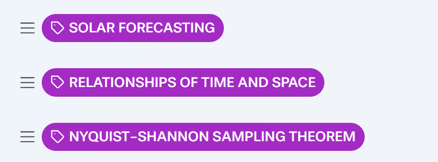
Grading
Yellowdig points you earn over the weekly point earning period (from Saturday to next Friday) will count towards 1000 pts. weekly target. But you can go above it (to 1350 pts. max). Yellowdig discussions will account for 15% of the total grade in the course.
Deadline
There is no hard deadline for participating in these discussions, but beware of the weekly limit. You need to create posts every week to stay on target with your total discussion participation grade. Each weekly point earning cycle ends Friday night, and a new period starts on Saturday.
8.8 Time Horizons of Interest
Reading Review
- J. Kleissl (ed), 2013. Solar Energy Forecasting and Resource Assessment. Elsevier Science, Academic Press. Read pp. 171- 177 from Chapter 8: "Overview of Solar-Forecasting Methods and a Metric for Accuracy Evaluation", by Coimbra, Kleissl, and Marquez
Electricity Markets and Grid Management
The first forecasts that we will explore from the reading are related to the modern electrical power grid. You are about to observe us jump from a +20 year time horizon in Lesson 7 (Life Cycle Cost Analysis), right down to spans of days and hours. If you recall from the reading by von Meier, this jump in orders of magnitude is pretty common for analysis related to financial and engineering decisions in energy systems.
Within the technological ecosystem of the grid, one follows the demand for electricity. Recall from Lesson 7 that the term for energy demand (including losses) is called the Load. Supply must be managed to match those dynamic demands. So, why might we forecast for loads in the electricity market? The time horizons of interest to engineers and financial experts working with the grid have been developed within the technical ecosystem of the modern power grid. When managing the grid as a dynamic system, we can think in time spans of seconds to minutes (Intrahour), over a few hours (Intraday), and over the course of a few days (Intraweek).
CAISO Example
Recall that California mainly has an Independent System Operator, with the exception of entities like SMUD (Sacramento Municipal Utility District). Also recall that an ISO uses markets (a zonal or nodal market) to manage the grid. In the last super graphic, which tied together weather scales and grid management scales, we observed "Hour Ahead" and "Day Ahead" markets along the top. But in our reading, we see that the time horizon is a bit different from the simple description:
- Day Ahead Market: Operational Day begins at 12:00a in the morning.
- Release load forecast at 5:30a in the morning of the day prior to the operational day. This means a +18.5h lead time from the beginning of the forecast. (5h:30 + 18h and 30 min = 24h)
- The forecast ends at ~11:59p of the forecast day. The end of the forecast is a +42.5h lead time from the end of the forecast that was initiated at 5:30a the day before. (5h:30 + 42h and 30 min = 48h)
- Hour Ahead Market: Operational Hour begins at the 0h.
- Release the hourly load forecast 1h and 45 min prior to the operational hour.
- Also release an advisory forecast with a +7h window from the beginning of the operational hour.
- Other Planned Markets: CAISO is considering intrahour forecasts for 5 minute intervals. Midwest ISO already does this.
- FERC: Notice of Proposed Rulemaking -- opportunity to schedule transmission every 15 min.
Time Horizons of Interest to Meteorologists
By reviewing the reading on Taylor's Hypothesis in Ch. 5 of the SECS text, we see that periods in time and distances can be related: a series of changes in time for a fixed place is due to the passage of an unchanging spatial pattern over that locale. So, in the following list, we can connect space and time (in fact, we do the same for power systems).
Taylor’s hypothesis permits a time series of irradiance observations over fixed locations to be converted into an equivalent translation across space (at the advective or propagation speed to the corresponding spatial pattern). Hence, all time scales are also spatial scales so long as the advective wind speed is much greater than the time scale of the evolving meteorological event being investigated, as is often the case.
-Brownson, SECS (2013)
Just keep this in mind with forecasting, as units of time actually also imply units of distance, and vice versa.
- Synoptic-scale weather: large-scale meteorology (also termed cyclonic-scale), with common atmospheric phenomena spanning 1000–2500 km (or days to month)
- Mesoscale weather: common atmospheric conditions spanning hundreds of kilometers (minutes to hours)
- Microscale weather: common atmospheric conditions spanning approximately 1 km (minutes)
Self-Check
8.9 Forecasting Summary
Reading Review
- J. Kleissl (ed), 2013. Solar Energy Forecasting and Resource Assessment. Elsevier Science, Academic Press.
The reading continues for pp. 177-182 of Chapter 8: "Overview of Solar-Forecasting Methods and a Metric for Accuracy Evaluation," by Coimbra, Kleissl, and Marquez [found on Canvas] - Optional: The sections following 8.2 (pp. 182-192) can be scanned for key topics rather than a deep read. 8.3 deals with metrics for evaluating models, which is a deeper statistical investigation than we have time for here. Also, those methods are still evolving in collaboration with meteorologists.
Forecasting
Reading Summary
A quick reminder, summarizing the reading from the previous page.
- >6 hour time horizon: physics-based models
- 2-6 hour time horizon: combination of methods via Numerical Weather Prediction (NWP) models
- <30 minute time horizon: apply ground-to-sky imager technologies
Events to be evaluated for <2 hours will use statistical approaches such as time series (Autoregressive Integrated Moving Average; ARIMA) or artificial intelligence (e.g., Artificial Neural Networks; ANN).
Meteorology-Specific Forecasts
As a slight correction from the reading assignment, we provide the following standard terminologies in meteorology for forecasting ranges, called lead times. These are not stated clearly in the reading, and they are important enough to have in your vocabulary. In the prior reading assignment, you should notice that the time horizons tied into solar energy models are not yet aligned with the approaches for meteorological forecasting. This is an indication of the relatively new start of forecasting applied to solar energy. We are still learning the common language of meteorology, and hopefully that language will soon converge. Similarly, meteorologists are beginning to adapt to the solar field's language of GHI, DNI, irradiation, etc.
- Medium-range: 3-7 days
- Short-range: 6 hours to 2 days
- Nowcast: 0 - 6 hours
- Hindcast: negative lead time
Numerical Weather Prediction (NWP)
Numerical Weather Prediction [206] uses an assemblage of modeling methods, along with current weather observation data to forecast weather in a future state. Note that the observations tied to the current state of the data are very important to NWP.
- Rapid Refresh from NOAA. [207]
- North American Mesoscale Forecast [208] (NAM) (mentioned in Table 8.1 of the reading).
Weather Research and Forecasting (WRF)
Local dedicated NWP models have been developed as a collaboration among NOAA and NCAR. The approach is termed WRF (pronounced "worf") [209]. This is an advanced application of NWP, but the skill with which one can forecast will still decay with increasing lead times due to the chaotic atmospheric behavior.
The Weather Research and Forecasting (WRF) Model is a next-generation mesoscale numerical weather prediction system designed to serve both atmospheric research and operational forecasting needs. It features two dynamical cores, a data assimilation system, and a software architecture allowing for parallel computation and system extensibility. The model serves a wide range of meteorological applications across scales ranging from meters to thousands of kilometers.
-WRF Homepage [209] (Accessed Oct. 20, 2013)
Research Occurring Now!
- Perez Research Group [210] at SUNY-Albany
- UCSD Solar Resource Assessment and Forecasting Laboratory [211] (Kleissl) and Coimbra Energy Group [212] (Coimbra)
8.10 Summary and Final Tasks
Summary
As a recap, in Lesson 8 we established that transdisciplinary research is a core part of integrative design, and while each of us doesn't need to be an expert in every field, we do need to stretch ourselves to understand and integrate our approach towards a common framework. In solar energy, that framework is tied to the goal of solar energy design and the foundations of sustainability systems. We then explored the role of risk and uncertainty in delivering solar resource units to the grid or managing the energy outputs on site, and defined risk as the dispersion of outcomes around an expected value, using the statistical variance of the data as a metric. Another way to explore dispersion from a banking and finance perspective has also been developed for renewables, using exceedance probabilities.
We then described the time-space relationship in both the grid, markets, and meteorological assessment. While there is still a lot to learn about the complex systems of weather, energy markets, and people demanding energy from the grid, we at least established a map to explore the scales of relevant time and distances using a general Earthly atmospheric advection speed of , which we dubbed the FRYB relation.
We explored the early methods to forecast solar energy metrics, and we found that some of the current limitations of solar resource forecasting are tied to the early nature of the field, while others are based in the general diminishing skill to forecast further into the future due to the chaotic nature of the Earth's atmosphere. We discovered that resolution limitations can be found in either spatial or temporal scales, too.
The relevant meteorological metrics for many common SECS technologies are tied into DNI, but we see that the field currently has very few methods to evaluate DNI to a high accuracy without directly measuring the parameter with expensive equipment. Finally, we note that most solar forecasts are linked to GHI only, which has limited value given our prior knowledge of the inherent error bound to Liu and Jordan-style transformations of GHI to and , and later POA for oriented arrays. These transformations also hold very little value to extract a meaningful DNI measure. This should be a reminder that the field of solar forecasting is still young, and we should be on the lookout for new progress that will enable us to minimize risk for our clients, hopefully increasing their solar utility in the respective locale!
Reminder - Complete all of the Lesson 8 tasks!
You have reached the end of Lesson 8! Double-check the to-do list on the Lesson 8 Learning Outcomes page to make sure you have completed all of the activities listed there before you begin Lesson 9.
Lesson 9 - Analysis for Policy Development
9.0 Overview
Overview
We now continue our development of broader impacts in systems design and management. So far, we have addressed the Goal of Solar Energy Design through engineering applications (Lessons 2, 3, 4) and through financial/economic applications (Lessons 5, 6, 7). In Lessons 8, 9, and 10 we are addressing the Goal of Solar Design by helping the client to manage risk in the given locale.
The Goal of Solar Design is to:
- Maximize the solar utility
- for the client
- in a given locale.
In Lesson 8, we discovered that there are meteorological phenomena that are really out of our control, and our job as a design and management team is to help the client to manage risk. Now, we continue with important design elements tied to managing risk, but within the social realm of community, regional, and federal stakeholders. In Lesson 9, we want to address helping our client to manage risk in the social environment, through our developed awareness of permitting and policy within the given locale. As we shall see, just because you have a good solar resource and a sound financial return (in principle), doesn't mean that the policies of the locale will allow one to actually implement a SECS, or to implement a system in a financially responsible manner.
9.1 Learning Outcomes
By the end of this lesson, you should be able to:
- describe the connections between policy making and renewable energy adoption at the local, regional, and federal levels;
- define the difference between solar rights and solar access;
- describe the role of net metering and permitting in solar project development;
- describe the leading methods for community solar development.
What is due for Lesson 9?
This lesson will take us one week to complete. Please refer to the Course Syllabus for specific time frames and due dates. Specific directions for the assignment below can be found in this lesson.
| Required Reading: |
J.R. Brownson, Solar Energy Conversion Systems (SECS), Chapter 11 - The Sun as Commons (Intro through "Framework: Emerging Local Policy Strategies") S. Bronin (2009) "Solar Rights" [213] Boston University Law Review. |
|---|---|
| Optional Reading (not required): | R. Knowles, "The Solar Envelope: Its Meaning for Energy and Buildings" [219], Energy and Builduings, 35, 15-25 (2003). |
| To Do: | Learning Activity: Community Solar Gardens Discussion: National Targets for Electricity Production No Quiz Assignment this week Engage in all Try-This and Self-check activities (not graded). |
| Topic(s): | Energy Policy Permitting Incentives Solar Rights Solar Access Community Solar |
Questions?
If you have any questions, please post them to the Lesson 9 General Questions and Comments Discussion Forum. I will check the forum regularly to respond. While you are in a discussion, feel free to post your own responses if you, too, are able to help out a classmate.
9.2 Solar Rights and Solar Access
Reading Assignment
- S. Bronin (2009) "Solar Rights" [213] Boston University Law Review. (only portions of the full paper are required reading)
- Introduction (all)
- Why Individual Solar Rights (all)
- Governmental Allocations (read the Intro; scan the sections on Permits and Zoning)
- Court Assignments of Rights (read the Intro)
- Conclusion (all)
- DSIRE Solar Portal [166]: Search by state, focusing on "Solar Access Laws". e.g., this Maryland Solar Easements and Rights Law [220].
- Wikipedia: "Solar Access" [214]
One of the main limitations to deploying solar energy is just the simple ability to make use of the Sun's energy. Here, we focus on the right to access and use the Sun's energy, and the functional ability to access unobstructed solar energy within the solar envelope. Try to remember that many technologies and objects that are outside serve as SECSs: homes and solar panels, yes, but also clothes lines, patios, and trees.
The DSIRE solar portal describes both solar rights and solar access (easements), along with a map of US states having each or both. Note that PA still has neither solar access laws, nor solar rights laws. The Wikipedia description is also a general framework to think about access to solar energy in society.
Context
Just think, in Germany, you have the right to be exposed to sunlight directly in any office scenario (no windowless cubicles permitted). In many states, you have the right to hang dry your clothes on a line outside. In ancient Rome, an individual had the right to access solar gains or be compensated for an obstruction of that resource. When we talk about policies for solar energy, one of the first is the basic ability to access that sunlight and then make use of it to do work!
The concept of solar rights is still emerging in the USA. I am going to recommend that you take about 10 minutes to review the current state of solar rights from the Solar America Board for Codes and Standards (the Solar ABCs [221]; choose 1 page summary). The coverage is brief but useful when considering the scope of solar legal status in the USA.
Solar Rights
The phrase "solar rights" is often used in a general sense and a specific sense. In general, solar rights are the broad class of legal rights to access and make use of the light from the Sun. In the specific sense, solar rights are distinguished from "solar access" by the following description:
- Solar Rights: the legal ability to install SECS on your property that is subject to land use restrictions. One of the classic SECS rights is the ability to dry your clothing outside on a clothes line. Perfect high utility SECS, but often blocked by local suburban covenants that would consider such displays as unwanted for the overall "appearance" of the neighborhood.
Here, solar rights describe the ability to make use of solar energy in your locale.
Solar Access
Solar access is the functional ability of a SECS within a locale to receive or "access" solar gains across property lines without shadowing or other obstruction occurring from buildings/trees/landmarks set in a nearby property. It also has to do with the enacted local policies to manage the commons of the solar resource system, and an individual's ability to be granted compensation if access is blocked in some way. Bronin has described solar access as being managed in three manners: as a solar easement, through covenants, and through lease agreements.
- Solar Easements: the legal ability for a property owner to use sunlight across property boundaries. Easements allow a designated landowner to hold some rights with respect to the property of another landowner. Such an easement will have been voluntarily bargained for and agreed upon. In such a case, one client will receive access to a solar corridor/envelope, while another landowner will receive some compensation to offset the burden from losing the access. [Bronin, 2009]
- Covenants: binding terms for current owners and those that follow later. A covenant can function well for newer subdivisions of homes, but they are more challenging to create for nonresidential regions or well-established residential areas. Of course, covenants have also been used to inhibit the use of SECS like clothes lines, foliage/tree types and density, and even visible displays of PV/SHW systems.
- Lessor-lessee arrangements: agreement that ties a solar right to the temporary term of tenancy. Solar leases will typically involve airspace (solar envelope or solar skyspace). Airspace has a common law role as real property, and is distinct from ground/mineral estates. A client owning property has the potential to sever the parcel of ground from the airspace, and then lease just the airspace. As such this type of lease allows the solar client to make use of or “occupy” the airspace without obstruction.
We have already discussed the role of minimizing shading in SECSs that intentionally collect and convert solar gains (rather than shading devices that attempt to control solar gains). Solar access has to do with access to the solar resource within the locale over many hours of the day, and across the months of the year. Recall that we already developed some skill to assess the solar access at a site through the sun path diagrams in Lesson 2. Hey, we just tied together something that was a lot of work earlier with an advanced topic in Lesson 8! Great!
Solar Envelope
The solar envelope is an extension of solar access, conceived for urban scenarios with a cluster of buildings and obstructions. Professor Emeritus Ralph Knowles of the Dept. of Architecture, the University of Southern California, conceived and developed an extensive exploration of the solar envelope as a concept for policy development and planning. You are welcome to read about Dr. Knowles' solar envelope concept in complement to our assigned reading.
Supplemental Reading
R. Knowles, "The Solar Envelope: Its Meaning for Energy and Buildings" [219], Energy and Buildings, 35, 15-25 (2003).
Self-Check
9.3 USA: Interstate Renewable Energy Policy and Permitting
Reading Assignment
- DSIRE Solar Portal: "Net Metering" [222]
- IREC/Vote Solar (2013) "Solar Permitting Best Practices" [215] (Accessed from IREC [223])
Net Metering
One of the more recent trends from the past decade of photovoltaic adoption is the ability to connect directly into the power grid. In such cases, policies have been adopted to allow renewable generators to "bank" excess power into the grid and receive credits for the excess energy (in kWh). But each locale will be subject to different policies enabling or prohibiting such practices. Net metering is expanding in creative ways, including aggregation of multiple distributed energy sources for credit, and distributing joint credit from a centralized solar garden [224] among multiple participants in a community.
Solar Permitting
Permitting is the unseen monster of project development that will slow or stop a project from moving forward. The key rewards of an established permitting process for SECS include reduced costs of installation and faster turnaround from design to deployment. It will be well worth your integrative design team's time to familiarize yourselves with the permitting process for your locale of interest.
Best practices have been itemized by IREC in our reading. We can distill those into a few core features that we would hope for in an integrative process that includes permitting:
- speed of processing (expedited processing, online processing);
- transparency of the process (requirements posted online and openly);
- reduced permitting costs (flat fee over value-based fees); and
- supporting permitting staff are knowledgeable of solar installations.
Self-Check
9.4 National Targets for Renewable Energy Portfolios
Reading Assignment
- REN21's Renewables Global Status Report (GSR) [216] (no, not the whole thing) (updated 2019):
- Please read the Chapter 3 Markets and Industry Trends, the section on Solar Photovoltaics (PV). If you have extra time, scan the review on CSP and Solar Thermal Heating and Cooling),
- review all Solar PV Figures addressing Global and Country Capacities and Capacity Additions.
- What are national and international targets for renewable energy integration, and where does solar fit in the portfolio? Up until now, we have really isolated our focus to the USA, but each country has a role to play in ramping up renewables in response to needed climate actions.
Different Countries, Different Approaches
So, first, "REN21" is the acronym for the "Renewable Energy Policy Network for the 21st Century". REN21 is a non-profit network of stakeholders established to connect key contributors from governments, international organizations, industry partners/associations, participants from science and academia, and society at large. We are using their centralized information base to expose the diverse approaches that countries can take to develop energy generation and manage energy demand at the Federal level.
After reviewing the REN21's Renewables GSR, you will have a little broader perspective on the various approaches, and will be able to compare solar policies in Germany vs. China vs. Columbia vs. Kenya.
9.5 Discussion Activity
Yellowdig Discussion - National PV Targets for Electricity Production
For this lesson discussion, do some online research on national targets for PV solar power. You can use the REN21 Renewables Global Satus Report [216] as a starting point, but certainly feel free to search other available resources. Take a look at different several key players representing different continents that are actively setting PV targets:
- Argentina
- India
- South Africa
- Australia
After reading and taking down some comparative notes, use these guiding questions to create your post in Yellowdig:
- What do these countries have in common with the choice of targets?
- How do their time horizons compare?
- Has there been a notable progress in these countries to achive these target?
- Can you speculate as to why these countries have large targets for PV, while other countries (e.g. Russia) do not?
- Whar are geographic, economic, and other prerequisites for setting renewable energy targets in these regions?
Tagging
Please feel free to use the following topics for your discussion posts this week:

Grading and Deadlines
Remember that Yellowdig point earning period ends each Friday. Posting commenting, reacting regularly through the weeek will make the 1000 pts. an easy target and guarantee a high participation grade in the course. Yellowdig discussions will account for 15% of your total grade.
9.6 The Sun as a Resource System and Common Pool Resource
Reading Assignment
- J.R. Brownson, Solar Energy Conversion Systems (SECS), Chapter 11 - The Sun as Commons (Read the Intro through "Framework: Emerging Local Policy Strategies.")
- J.R.S. Brownson (2013) "Framing the Sun and Buildings as Commons" [217]. Buildings 3(4), pp. 659-673; doi:10.3390/buildings3040659.
I want you to consider the perspective where we view the resource units derived from the sun (light, converted electrons, converted heat, etc.) and the resource systems to enable those conversions (the Sun, the grid, our buildings) as coupled, but separate entities. This is an extension of our work on economics, but leads us into thinking about management of solar energy among the community.
While reading these materials, think how we might collectively manage both the resource units, and the resource systems in a given locale. Community solar is a new and exciting space in the solar field, and this sets up the foundation to address it and think of new strategies in management.
Language of the Commons
In both readings, we are going to see the language developed by Nobel Laureate in Economics Elinor Ostrom, from her seminal book, Governing the Commons: The Evolution of Institutions for Collective Action.
- Resource Systems: the larger stock from which a good is appropriated.
- Resource Units: the flow of goods being produced.
- Providers: teams or individuals who arrange for the provision of a resource system at multiple levels, to ensure long-term stability or sustainability of the resource system.
- Producers: teams and individuals who construct, commission, and maintain access to the resource system.
- Appropriators: individuals who make use of resource units.
- Arbiter: a third party, as either an impartial person or an institution, that is given the power to decide among stakeholders in a controversy.
From this, we state that the Sun is an energetic resource system providing the flow of light (as resource units) in the shortwave band (280–2500 nm). Once we have established our language for resource systems and resource units, we can review the Typology of Goods, discussed with examples in the article by Brownson (2013). We summarize those four main goods below:
- Excludable Goods: restriction of access to the good. High excludability means access to the good can be intentionally restricted, while low excludability means one cannot easily restrict access to the good.
- Rivalrous Goods: when the appropriation of a good takes away from another’s ability to appropriate that good (called subtractable). High rivalry means that the goods are subtractable (independent of excludability), while low rivalry means that subtraction of a unit of the good does not take away from the ability of another to use the good.
- Private Good: when a good is both rivalrous and excludable.
- Public Good: when a good is both non-rivalrous and non-excludable (really big resource systems like the Sun).
- Club Good: when a good is non-rivalrous and excludable.
- Common Good: when a good is rivalrous but non-excludable.
Self-Check
9.7 Community Solar
Reading Assignment
NREL Report: J. Coughlin, J. Grove, L. Irvine, J. F. Jacobs, S. Johnson Phillips, A. Sawyer, and J. Wiedman (2012) "A Guide to Community Shared Solar: Utility, Private, and Nonprofit Project Development" [218] USA DoE National Renewable Energy Laboratory.
- Read Sections 1 and 2 (pp. 2-32)
- Scan through Section 3: "Emerging State Policies to Support Community Shared Solar" and Section 7: "Resources"
Models of Community Solar
Our final reading puts a few boundaries around the varieties of "community solar" that appear to be emerging in the USA of late. There are good examples in the document, which will be helpful for our Learning Activity in this lesson.
- Utility-Sponsored Model: A utility owns or operates a project that is open to voluntary ratepayer participation.
- Special Purpose Entity (SPE) Model: Individuals join in a business enterprise to develop a community shared solar project.
- Nonprofit Model: A charitable nonprofit corporation administers a community shared solar project on behalf of donors or members.
While community solar PV is just now emerging onto the market, note that community solar products have been in existence for millennia as shared fields and gardens for produce development and resale. Based on the prior examples from farming, the management of a community resource is well within the scope of SECS expansion.
Community Solar Case Studies
As of 2020, Community Solar is now authorized in 19 states and Washington, D.C. There are companies that specialize in community solar that would arrange deals with farmers to lease portions of their land to build solar projects. As this segment of the solar industry expands, farmers (and landowners in general) may take advantage of this new revenue stream. In addition to generating local revenue, solar projects help states make progress toward their clean energy and sustainability goals [Gahl, 2020].
Browse through this report to learn about several representative community solar case studies across the country:
SEIA Report: Gahl, D., How Community Solar Supports American Farmers [225], SEIA, February 2020.
The case studies presented in the report show that typically, farms will lease portions of their land to community solar companies for a fixed term at a fixed price. These solar lease payments tend to be higher than those for traditional agricultural operations and are normally based on the state policies, where the project is located. Land leasing for solar often provides farmers with higher and more stable income than that obtained through producing agricultural products, which creates an incentive.
9.8 Learning Activity: Community Solar Garden
Scenario
Imagine you are part of a superior design team based in PA, a state with a restructured electricity market such that community solar is possible. Your integrative design team is already capable at commercial and residential PV installations, but wants to branch out and take advantage of this "community solar" concept. Your job is to make a short survey of best practices available elsewhere and suggest a model for developing community PV in an urban community in the Philadelphia area. Understandably, your report would be based on limited information of the actual site, but you can leverage extensive access to general information about the types of building and potential stakeholders in the locale of interest. Based on your findings, you need to prepare a concise but convincing summary document for your supervisor to review.
Directions
- Find and review a case of community shared solar anywhere that would align with a prospective community solar scenario in Philadelphia area. Make sure to state the commonalities in that real case with those in the potential project scenario.
- Develop a 2-3 page executive summary that includes:
- background information of the locale,
- client base and stakeholders,
- proposed model for community solar,
- comparative analysis (cons and pros) for community solar vs. individual solar. (If you like, you can present this information in a table).
- Provide a conclusive statement about the feasibility and benefits of the project.
Submission
Submit your Summary as a PDF document into the Lesson 9 Learning Activity Dropbox: Community Solar in Canvas. Remember to appropriately cite any sources of information used in your report.
Grading Criteria
You will be graded on your ability to develop a compelling outline that provides scope for applying the community solar concept in a residential Philadelphia neighborhood. The activity assesses your knowledge of investigating the potential client and stakeholders at the locale when planning to maximize solar utility in the pre-design phase. Please see specific grading rubrics in Canvas.
Deadline
Please see the Canvas Calendar for specific due dates.
9.9 Summary and Final Tasks
Summary
In this lesson, we attempted to flesh out some major policy topics tied to solar energy. In doing so, we were able to describe the connections between policy-making and renewable energy adoption at the local, regional, and federal levels. We explored the deeper meanings and implications of solar rights and solar access, which engage multiple stakeholders from a local and regional government. Then, we addressed the policy and permitting barriers/opportunities in solar project development.
Recall that we want to help our client to manage risk in the social environment, through our skill in negotiating permitting and policy barriers within the given locale. A good solar resource and a sound financial return (in principle) alone doesn't guarantee the locale will even allow a SECS, or to implement a system in a financially responsible manner.
The research of Dr. Ostrom suggested to us how local community action for solar energy is not only possible but is actively used today in other similar industries, where the dynamic appropriation and provisioning challenges of a resource system and resource units are addressed in a sustainable fashion. In turn, we used that thought process to describe new and expanding methods for community solar development.
Reminder - Complete all of the Lesson 9 tasks!
You have reached the end of Lesson 9! Double-check the to-do list on the Lesson 9 Learning Outcomes page to make sure you have completed all of the activities listed there before you begin Lesson 10.
Lesson 10 - Ecosystems Impact from Solar Land Use
10.0 Overview
Overview
This is our last lesson of three that are tied to the broader impacts of solar design. In Lessons 8, 9, and 10 we have been addressing the Goal of Solar Design by helping the client to manage risk in the given locale. This lesson deals with risk in terms of uncertainties that are encompassed in the long-term time horizon of projects as they have societal and environmental impacts.
Sustainability plays a major role in focusing our views of solar energy deployment and managing long-term risks (generational time scales). This lesson tries to encompass those broader impacts of developing a renewable energy project and addresses the motivation for sustainability system thinking in project design. We frame this lesson in terms of sustainability ethics and ecosystems services, and we will develop our activities in this lesson around discussions and essays. You will be using the answers from your Learning Activity to inform the broader impacts section of your final projects.
We are often reminded of how energy technologies, when deployed on a large scale (natural gas, oil production, coal combustion, etc), will have significant environmental impacts that are disruptive to the global, regional, and local ecosystems. I want you each to consider how large-scale solar energy deployment can also induce ecosystem change and reduction in ecosystems services, which must be avoided in future project development. This lesson will build upon the Millennium Ecosystem Assessment [226] that was called for in 2000 by the United Nations.
10.1 Learning Outcomes
By the end of this lesson, you will be able to:
- describe how sustainability ethics can be included into project design as a motivating factor for Solar Project Development;
- apply the four classes of benefits that are supplied by ecosystems: ecosystems services;
- apply the concept of ecosystems services to renewable energy projects in rural and urban scenarios; and
- become familiar with the context of the Millennium Ecosystem Assessment [226]
What is due for Lesson 10?
This lesson will take us one week to complete. Please refer to the Course Syllabus for specific time frames and due dates. Specific directions for the assignment below can be found within this lesson.
| Required Reading: |
J.R. Brownson, Solar Energy Conversion Systems (SECS), Chapter 1 - Introduction (Reread, with renewed focus on The Ethics of Sustainability and Ecosystems Services.) Geoffrey Carr (Nov 21, 2012) "Sunny Uplands [227]" The Economist. |
|---|---|
| Optional Reading (not required): |
"Ecosystems and Human Well-being: General Synthesis" (Millennium Ecosystem Assessment site page [231]) (155 pg. report [232]) Ong et al. (2013) "Land-Use Requirements for Solar Power Plants in the United States [233]" [13] NREL Technical Report: NREL/TP-6A20-56290. (supplemental reading) |
| To Do: |
Discussion: Ultra-Mega Solar Activity: Sustainability and Ecosystems Services Pitch (video) Engage in all Try-This and Self-check activities (not graded) |
| Topic(s): | Energy constraint, value of solar energy, historical cases of developing solar energy |
Questions?
If you have any questions, please post them to the Lesson 10 General Questions and Comments Discussion Forum. I will check the forum regularly to respond. While you are in a discussion, feel free to post your own responses if you, too, are able to help out a classmate.
10.2 Exponential Growth of Solar and Impact
Reading Assignment
- Geoffrey Carr (Nov 21, 2012) "Sunny Uplands" The Economist [227]. (Yes, it still holds true years later...)
- Doubling Time [228] (Wikipedia article, accessed on Nov. 14, 2013)
Please read about the rate of growth of PV (it's been quite high for decades), tied to the "learning curve" of PV costs from a doubling in cumulative production capacity. There is a positive feedback loop occurring here, and it suggests that PV (and other solar) will become very, very big globally within the next decade.
Growth in Solar
From our reading, we have seen the:
- Growth Rate: 32-37% increase in PV installed globally:
- PV industry as installed capacity (in Wp) doubles about every 2 years (or less in recent years).
- Compare this to the (still large) rate of growth of wind capacity from 2006-2016: 17-18%.
- Swanson Effect: 17-24% drop in manufacturing costs (called a learning curve or an experience curve) with each doubling of cumulative production (learning curve):
- Installed capacity is different from the time for cumulative production to double (2-3 years), but it is similar.
- \$76.67/watt in 1977 to \$0.74/watt for 2013.
- Growth rate combined with the learning curve is a positive feedback loop in systems thinking. Meaning: "more solar" will lead to "a lot more solar!";
- With every doubling, the awareness of other solar technologies increases. e.g.:
- CSP from Ivanpah Solar Power [234]
- Solar thermal processing in Austria (brewery) [235]
- Solar seasonal home heating in Drake's Landing [236], Alberta, Canada; and
- Even the building industry shares a solar history through passive solar architecture [237].
Self-Check
10.3. Scale of Solar and Ecosystem Services
Reading Assignment
- B. I. Cook, R. L. Miller, and R. Seager (2009) "Amplification of the North American "Dust Bowl" drought through human-induced land degradation." [229] Proceedings of the National Academy of Sciences of the USA. 106(13), 4997-5001.
- Ong et al. (2013) "Land-Use Requirements for Solar Power Plants in the United States" [238] NREL Technical Report: NREL/TP-6A20-56290. (supplemental reading)
Now we are going to tie our focus on scale to ecological impact. This reading is complementary to the concept of solar energy. Consider that large scale solar is called a "solar farm" or community scale solar can be termed "solar gardens." Large scale farming leads to large scale land use changes, and may undermine environmental resilience and existing ecosystems services.
Scale of Solar: Now and in the Future
We keep hearing about exponential growth of the solar industry, and larger and larger SECS projects are being rolled out each year. Solar consumes a lot of land, so here we especially focus on the impacts that come with major land use changes. Consider how the land use of these solar projects is linked to the observed ecological disruptions.
Gujarat Solar Park [239] in Gujarat, India:
- Only began installing in 2011, and nearly 1,100 MWp of PV completed as of 2016.
- Chankara Solar Park [240] consumes the largest area: 4,900 acres (19.8 km2 or 7.7 mi2); eventually host 500 MW of PV (an average of 9 acres per MW installed, or 25 MW for every 1 km2).
- This is very, very fast development of power.
- Neighboring state of Rajasthan, India is planning for 4000 MWp of solar power in the near future.
Ivanpah Solar Power Facility [234]:
- CSP power tower systems installed in California/Nevada border of the Mojave desert.
- Unit 1 of 3 was connected in September of 2013.
- Three solar thermal power stations will consume 4,000 acres (16 km2 or 6.25 mi2) to host 392 MW of power (an average of 24.5 MW per km2).
- The process was relatively rapid (over the course of 3-5 years), but the CSP plants take longer to install than PV (however, PV does not have evening power storage).
- Disturbance of the land in the northeastern Mojave Desert (the Ivanpah Valley) was significant to a threatened species of desert tortoise. This lead to a relocation of tortoises [241] by the developer, BrightSource Energy, Inc.
- The Solar Energy Industries Association describes the Department of the Interior's process associated with the large land permitting process [242].
These very large solar projects (4,000-5,000 acre scale), started around 2012, are now considered "medium scale”, given the doubling time of PV capacity. There are now Gigawatt scale solar farms in development, with one near Tibet at Longyangxia Dam Solar Park at 850 MW scale (see satellite images from NASA [243]). So the expected ecological impacts will be even more dramatic and may result in not only local, but regional and global consequences.
Furthermore, the direct land use impacts (such as clearing or changing the land for solar installation) is only a trigger for a larger scale land impact. The Dust Bowl [244] of the USA in the 1930s was initiated by the land use changes of only about 1000 acres in marginal lands, but eventually affected 100 million acres (400 thousand km2). System causal connection and feedbacks within natural ecosystems propagate the initial disturbance to a greater territory and over a greater period of time.
Recognizing the challenge of cultivating marginal arid land, the United States government expanded on the 160 acres offered under the Homestead Act—granting 640 acres to homesteaders in western Nebraska under the Kinkaid Act [245] (1904) and 320 elsewhere in the Great Plains under the Enlarged Homestead Act [246] (1909).
-Dust Bowl [244] (Wikipedia entry, accessed Nov. 15, 2013)
Ecosystem Services
Significant land areas are being designated for solar projects, including both natural and partially developed. However, the solar development does not have to be detrimental to the health and values of local environment. As well as providing low carbon energy, solar farms can also provide important benefits for biodiversity and ecosystem services. Furthermore, land use change for solar installation presents an opportunity to address the urgent challenges of mitigating ecosystem degradation. In other words, degrading lands can be brought back to health.
However, given the high rate of solar industry development, it is an important time now when we need to determine the best ways to design and manage utility scale solar plants. In fact, many solar projects are built on low-grade or otherwise intensively managed agricultural land and may create an opportunity to enhance biodiversity and return the fields to a natural state.
Let us then review the main types of ecosystem services we are talking about here.
- Provisioning: Things that we get from the ecosystem: food, water, fresh air, wood, medicines, and other natural resources that fulfill our primary needs.
- Regulating: Processes in the environment that regulate climate, water cycling, and purification, waste degradation, pollination for crops, soil erosion control, pest control, etc.
- Cultural: Non-material aesthetic and recreational values we get from being in nature: e.g. views, hiking trails, fishing lakes, national parks, etc. These will support our emotional well-being and mental health.
- Supporting: Resources that support all the above services: habitat, flora and fauna, biodiversity, and soil.
There are sometimes no distinct boundaries between these types, as the same resource may be considered within several categories. For example, trees or soil can be both part of supporting system and provisioning products. Or another example is storing carbon in biomass can be both regulating (carbon sequestration) and resource generating or provisioning (fossil fuel).
At the stage of solar project design, we may want to take a close look at the ecosystem services existing in the target area and assess their environmental significance for the local community. Next, we may want to plan measures and design features that either have minimal impact on those services, enhance them, and add additional value. At the same time, we may want to avoid the actions or design features that are detrimental.
Try This! SPIES Tool.
A Group of researchers at the Universities of Lancaster and York (UK) developed an online tool – “Solar Park Impacts on Ecosystem Services" (SPIES) – that helps practitioners make informed decisions on solar design and environmental management. This tool is evidence-based, so all the impacts and strength of the impacts associated with different projects activities on site are researched and referenced. SPIES compiles 457 peer-reviewed academic articles collected via a systematic review of relevant issues.
The interactive interface allows users to arrange scientific evidence by ‘ecosystem service’ and to generate a list of management interventions that will affect the achievement of a desired environmental outcome.
The SPIES tool can be used for planning applications by showing how solar projects can contribute to the environmental and biodiversity targets, if managed properly. The options presented by SPIES can help developers decide which ecosystem enhancements will be the most appropriate for the particular locale. This tool can also be useful to local authorities and policy makers who are required to consider environmental benefits and risk and approving project proposals.
Go to the SPIES website: https://www.lancaster.ac.uk/spies/ [247]
Scroll down to the bottom and click to download the SPIES tool – you will receive the login information for using the database. Feel free to check out other supporting resources.
Hope you find it useful in your own development!
10.4. Sustainability Ethics as Part of Solar Projects
Reading Assignment
- SECS, Chapter 1 - Introduction (re-read, with renewed focus on The Ethics of Sustainability and Ecosystems Services)
- C. Becker (2012) Sustainability Ethics and Sustainability Research, Chapter 3 - The Inherent Ethical Dimension of Sustainability – Toward a Relational Ethical Perspective (available on Canvas) pp. 17-20.
Sustainability Ethics
The major work of research on ecosystem services came out of the Millennium Ecosystems Assessment [231] from the United Nations. Even the synthesis report is a heavy read, so we have included it as supplemental reading. Here is an excerpt from the report that I considered to be highly appropriate in the context of developing large scale solar technologies globally:
Relationships between Ecosystem Services and Human Well-being (p. 49)
"Changes in ecosystem services influence all components of human well-being, including the basic material needs for a good life, health, good social relations, security, and freedom of choice and action (CF3). (See Box 3.1.) Humans are fully dependent on Earth’s ecosystems and the services that they provide, such as food, clean water, disease regulation, climate regulation, spiritual fulfillment, and aesthetic enjoyment. The relationship between ecosystem services and human well-being is mediated by access to manufactured, human, and social capital."
This statement is closely linked to the "sustainability ethic" - the term that has been eloquently summarized by Dr. Christian Becker (former faculty in the PSU Department of Philosophy, and expert on sustainability and ethics) as the following:
"Acknowledge and seek solutions that respect a systemic and simultaneous moral obligation to 1) contemporary global communities, 2) future generations of human society, and 3) the natural community or environment supporting life and biodiversity on Earth."
We can see that this invokes a pretty deep perspective, and there is a lot of value encompassed within such a concise statement. I want you to consider several ways of how we might incorporate the sustainability ethic as a motivator into our working lives as professionals.
- Embody your own conviction that corporate interests can be reconciled with social and environmental interests.
- Advocate public participation in the decisions that affect environmental justice.
- Make a business case for sustainable practices in the context of a particular energy business or utility.
Case Example: Keystone Solar Project
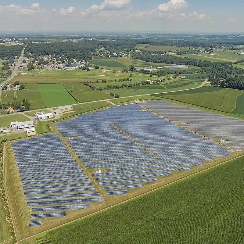 |
(Image Credit: Community Energy [248]) |
The folks at Community Energy [249] and EDF Renewables [250] in Pennsylvania have developed just such an approach to project development, in their Keystone Solar [251] project. This 6 MW PV project was developed on Amish farmland, with specific research applied to the soil quality before and after the project installation. No concrete was used in the ground mount installation here. The design included vegetative buffering with native grasses, shrubs, and trees, allowing the solar installation to blend into the natural landscape. The project received a Project of Distinction Award at the 2013 PV America East Conference.
Several universities and other organizations signed up for a share of the renewable energy credits, including Drexel University, Franklin & Marshall College, Eastern University, Clean Air Council, the Philadelphia Phillies, Juniata College, Millersville University, and Marywood University.
Video: Keystone Solar Time-Lapse (:54)
Best practices were applied, and at the end of the contract employing the solar farm, the land owner will have the option to remove the entire installation and return the land back to farmland for agricultural crops. This is still not the norm in the industry, it is a best practice by a firm seeking to lead the industry.
Case Example: Penn State - Light Source BP 700 MW Solar Farm
“ UNIVERSITY PARK, PA. — On Feb. 5, 2019, Penn State and Lightsource BP announced the development of a large-scale, ground-mounted solar array of over 150,000 solar panels near Penn State’s Mont Alto Campus. This 70-megawatt, off-site solar energy project will support the University’s Strategic Plan, helping implement the plan’s "Stewarding Our Planet’s Resources" key pillar and supplying up to 25 percent of the University system’s electricity.” (Verdi, 2019 [254])
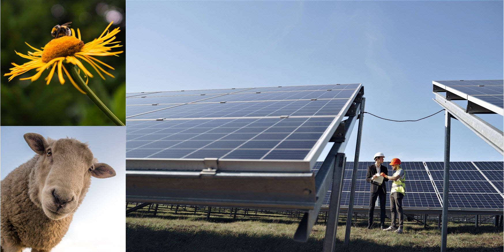
|
|
This project boasts significant environmental benefits due to shifting the campus electricity generation from fossil fuel based to renewable sources. It is estimated that, once implemented, the project will result in 57,000 metric tons of avoided CO2e emissions per year, which is equivalent to 12,102 fuel-burning cars of the road. The project helps Penn State exceed its goal of reducing carbon emissions by 35% by 2020 and also provides the university with $14M in energy cost savings over the 25-year term of PPA agreement. But that is not the end of it. From the very start, the intention was to demonstrate that utility-scale solar can be and should be developed in a sustainable way, with careful consideration of local ecological values.
The bidding process required developers to evaluate the potential impacts on the land and nearby ecosystems by using a mapping tool developed by The Nature Conservancy (TNC) [259], a global environmental non-profit organization that advocates responsible use of land and sets priorities for conservation of sensitive and ecologically critical zones across all continents.
Lightsource BP is recognized for building solar farms that enhance environmental benefits to farm lands, preserving biodiversity and agricultural value of land. They worked together with Penn State’s researchers to come up with “environmentally-conscious” system design, which included elements, such as created wildlife habitats, plant communities that promote pollination and help uphold honey bee population, and sheep grazing (Ludt, 2019 [260]). By design, the solar farm allows for co-location of the traditional agriculture benefits (crop and livestock growing) with additional ecosystem services.
The construction of the plant has been completed in 2020, and Penn State announced in October 2020 that the university had begun purchasing solar electricity:
Video: Penn State and Lightsource bp Virtual Ribbon Cutting Event | Lightsource bp USA| Responsible Solar(12:28)
On-screen text: Welcome to our virtual ribbon-cutting ceremony. As of October 2020, Lightsource bp’s Nittany 1, 2 and 3 solar farms are generating renewable energy for all Penn State Campuses.
Eric Barron: Greetings! Last September Penn State and Lightsource bp celebrated the groundbreaking for a 70-megawatt solar project in Franklin county that would provide twenty-five of the University's total purchased electricity over twenty-five years. One year and one month later it's my pleasure to share that the project is complete, and Penn State is purchasing this renewable energy through a power purchase agreement. This is a bright and proud moment for Penn State and reminiscent of a day in April 2018 when I loaded the last shovel full of coal into the University power plant Penn State's commitment to renewable energy helps us reduce our greenhouse gas emissions and energy costs but the value of successfully completing projects like these extends far greater than achieving these two goals. Through these efforts from planning to implementation and beyond our students are granted first-hand, once in a lifetime access to innovative learning and research opportunities related to the expanding renewable energy industry. These living lab experiences prepare students for new career possibilities and a brighter future for all of us. Thank you to everyone who has worked so hard to make this possible.
Kevin Smith: Hi, my name is Kevin Smith, I’m CEO of the Americas for Lightsource bp. Lightsource bp is a large-scale solar energy development company with activities around the world. As CEO of the Americas, I head up our US activities developing, investing, and building large-scale solar projects here across the US. I want to take a moment really to congratulate the Lightsource bp team and the Penn State University teams for really a terrific project here that's now completed construction and has started to generate a clean and cost-effective energy for Penn State University and the 100,000 students that they have across Pennsylvania. This is really a great example of what we would call responsible solar energy, so not only does it have cost-competitive energy, clean energy, created jobs during the construction period, and continued investment in the community through our expenditures on maintenance activities on the facility as we move forward. But it also provided uh some other community benefits um you know one of which is diversification of revenue streams to some of the farming community. So, some of the farmers that participate in the project um now have a long-term, safe, solar solar energy generated revenue stream to pair with their farming activities as well so provides them with that additional benefit of nice secure long-term revenue streams. In addition, we really looked at how to harmonize this project with nature in the area and with the farming community. That included the creation of habitats for wildlife and included a pollinator program with a custom seed mix to make sure we're developing the proper wildflowers in the area to help with pollination activities and in addition, we're going to be doing sheep grazing on one of the sites that we have here in the project you know. This work really came out of the shared goals that we have with Penn State University, they were very specific in their requirements for a project that they were going to be buying electricity from, and fortunately, this was really a core principle for Lightsource bp and our projects around the world is to develop these kinds of activities. It's been a great experience with Penn State University Meghan and Rob and President Barron and the whole team have been really wonderful to work with, really drove the requirements for the project and we look forward to continuing that relationship for decades to come. We have a number of interns that have been working with the company and we expect that will continue as we move forward -- looking at special projects not only for us but also for the University as they now have this large-scale facility at their doorstep where they can do investigations on all kinds of activities. Not only pollinator programs but also battery storage potential and other things. So anyway, we really look at this as a model project for us, and as does Penn State and we look to implement a lot of the things we learned on this project on our projects across the US. So, once again congratulations to the Penn State team and to the Lightsource bp team we look forward to a long and exciting relationship with Penn State as this project continues to go forward and generate electricity into the system. Thank you very much.
Rob Cooper: Hi, my name is Rob Cooper, I am the senior director of energy and engineering for the office of physical plant at Penn State. Since they began looking into solar years ago and have since learned so much about the value of renewables through our participation in this project. We have learned that utility-scale solar located in Pennsylvania can provide cost savings when compared to fossil fuel and nuclear power generation sources. We have learned that renewable projects can create jobs and generate supplemental income for farmers. We have learned that carefully designed and constructed solar projects can also improve local habitat and biodiversity and we have learned that these types of projects provide a valuable educational opportunity for Penn State students through research potential and student internships. Moving forward this experience will guide Penn State as we evaluate future opportunities to continue to lower our carbon emissions and make Penn State more sustainable.
Emilie Wangerman: Hi, my name is Emilie Wangerman and I lead Lightsource bp's business development organization. So, I have had the pleasure of working with Penn State throughout this whole process. I started with selecting the projects which we would submit into the RFP process which was well run and thoughtfully organized throughout the process. I really appreciated the questions that were asked and the focus on not only driving forward affordability for Penn State but also caring about the impact to the community and to the environment and the good news is that our projects were well paired to be selected and therefore move into negotiations which I did throughout the process with an amazing group of people at Penn State. Thanks to Rob and to Mike, both of you were a pleasure to work with, and then I had the opportunity to work with Meghan and others to really define what are the added benefits beyond the procurement process and that included things like internships and opportunities to engage in research. This is a great example of an RFP process that really can be a blueprint for other universities throughout the US and globally it's a great opportunity to find affordable clean energy and procure it in a way that you can ensure that you're getting a quality product. Overall, it was an exciting opportunity I look forward to the continued long-term partnership with Penn State, and overall, it's a great way to bring about a continued growth in the renewable energy market through a public and a private partnership. So congratulations to everybody this is an exciting time and I’m really proud that these projects are online and producing clean energy for Penn State.
David Dosker: Hello, my name is David Dosker and I’m the Lightsource bp project director for the Nittany one, two, and three solar sites. As the project director for Lightsource bp I’m responsible for the planning and construction of the Nittany sites. Over the last year and a half, it has been my honor to work with Meghan Hoskins and the Penn State team. Both Lightsource bp and I are proud of the relationships and the facilities that we have built together, we are excited that the Nittany sites will continue to provide benefit to Penn State the community and to the environment for years to come. Congratulations to Penn State and Lightsource bp as we start this amazing energy journey together.
Meghan Hoskins: Hello, I’m Meghan Hoskins at the Penn State sustainability institute. This solar project has been unique in many ways, but I'd like to give you a couple of quick examples of collaboration efforts among partners of the project that have made it really special. One of Penn State's priorities for the project was to share the story of how large-scale solar projects can be developed in a way that benefits the local community and environmental resources surrounding the project. We achieved this through a partnership with the association for the advancement of sustainability in higher education: where we produced a webinar that highlights the process that Penn State went through to involve partners like the nature conservancy and Lightsource bp to achieve our goals of responsible environmental stewardship. That webinar is accessible to anyone and we hope you'll go check it out. Another goal we had was to make the sites available not only to the humans in the neighborhood and at Penn State but also as habitat for local wildlife as a company who shares our goals of improving local ecology, Lightsource bp partnered with a local farmer who will graze sheep on one site and also planted a seed mix around and under the arrays that was recently designed by other partners to support not just sheep but also insects, a seed mix, appropriately named fuzz and buzz.
Mark Chambers: Hello, everyone Mark Chambers, senior construction manager for Lightsource bp. So, I’m back in the fieldwork until it started, over here at solar one. I have to say this has been a really interesting journey with everything that's going on, great people, meeting the Penn State faculty and students, very smart, really good questions but I have to say that one big thing is that with these interesting times is realizing the perseverance of what the team had to get it done. We have a great crew, finished, and provided three safe quality clean energy generation projects. These were the first for us with Penn State, hopefully not the last and see you at the next one in the meantime please be safe, take care, and go lions!
David Gray: thank you for joining us as we celebrate this important moment in Penn State's history. In January of 2019, I was genuinely enthusiastic to sign on behalf of the University, a solar-powered purchase agreement with Lightsource bp to build the largest solar array in Pennsylvania. Through this initiative, Penn State is doing good and doing well simultaneously. We're doing good things for future generations by reducing dangerous greenhouse gas emissions that contribute to climate change we're doing well for the University by producing a positive return on investment that will yield millions of dollars in net present value savings for Penn State. At a time when we are facing so many great challenges, the beginning of this 25-year power purchase agreement offers a bright moment and a true reflection of the University's ability and commitment to not just grow but to succeed in a way that enhances the health and sustainability of the planet and future generations this project has involved countless Penn State students, faculty and staff along with industry professionals but its positive impact will reach all of us. When Penn State reduces its carbon emissions by utilizing more renewable and affordable energy, we all win! This is just one example of how Penn State prioritizes doing well while doing good and just one reason why I am so proud to be a Penn Stater. We are Penn State! And we are doing great things for the environment. Thank you!
More facts about the project:
Penn State: Power by the Sun, Lightsource BP – Penn State Brochure 2020 [263].
The latest announcement of project commission:
Penn State Powers Up with Solar [264], BusinessWire, 10/15/2020.
Try This! Explore Resilient Land Mapping Tool
This web tool provides you with several metrics and interface to evaluate the environmental sensitivity of a region or site. If you consider developing a tract of land or re-purpose a natural area or farmland for solar installation, it is important to access the potential impacts on biodiversity, water ways, soil, species migration routes, and other factors. For example, it may help you to choose an area with the highest resilience or avoid areas that are prioritized for conservation.
First, it is helpful to understand the core concepts of terrestrial resilience. Visit this webpage [265] to study the metrics used in mapping.
Resilient Land Mapping Tool [266]
Zoom in the location of your interest. There are several options on the right hand menu to display different metrics on the map: Resilient Sites, Connectivity and Climate Flow, Recognized Biodiversity Value, and Resilient and Connected Network. You can try to switch between the options and interpret the markings based on the legend at the bottom of the menu.
Then try to “Sketch a Polygon” over a specific site (see button on the upper right). In a minute, the system will generate a profile report for that site, which gives you some quantitative information on ecological sensitivities in this area.
Think how this information can help you make a case for sustainable solar project. Feel free to use this tool for site assessment in your course project.
10.5 Ecosystems Services in the Urban Environment
Reading Assignment
- D. Ervin, D. Brown, H. Chang, V. Dujon, E. Granek, V. Shandas, and A. Yeakley (2012). Growing Cities Depend on Ecosystem Services. [230] Solutions, Vol 2, No. 6. pp. 74-86.
Urban Ecosystems
Portland State University of Oregon, USA, has developed an IGERT (Integrative Graduate Education and Research Traineeship; federally funded graduate research) on "Ecosystem Services for Urbanizing Regions." They have clearly identified our urban ecosystems as essential as well. Looking at the summary of content from our reading, we should note how closely it all aligns with the integrative design approach in our own text book.
- The global human population living in urban regions: >50% (projected to grow by 2050). This urban-centered ecosystem will intensify pressure on ecosystems that support urban areas.
- Wicked problems [267]: generated by urban population pressure on ecosystems, and their services, require integrative solutions (transdisciplinary) that include multiple fields of study and practice.
- Best practices: formed through collaborations among multiple organizations: nonprofit, public/government, and private.
- Integrative design: collaboration where all relevant stakeholders are brought into the processes of problem scoping, design, and implementation.
- Requires innovative education: to train future scientists and managers in integrative problem-based strategies and design for critical challenges in ecosystem management.
Now, how are you going to think about urban ecosystems services in your own solar design projects?
10.6 Discussion Activity
Yellowdig Discussion: Ultra-Mega Solar - Sambhar Lake Study
Now that we have seen indicators of the growth of solar globally in both rural and urban regions, let us discuss the ultra-mega solar project that was proposed for India...which was ultimately stopped and shifted to the state of Gujarat due to environmental concerns! Let us set the stage as if we were in 2013:
- "India to set up world's largest solar project near Sambhar lake in Rajasthan" [268]Press Trust of India. Sep 21, 2013 at 02:24pm IST
- "India's Plan for World's Largest Solar Farm May Stumble over Wetlands [269]", Saket S., The Guardian, 2/11/2014 (Accessed Nov. 14, 2022)
- Rajasthan, India [270]: the nearby location is Sambhar Lake [271] (a salt source for the state) and Jaipur. [272]
- 4 GW centralized solar power, but it is not clear if it will be PV or CPV or CSP.
- What is there now? Dhirubhai Ambani Solar Park [273]: much less than neighboring Gujarat.
- Search any recently published information on this case.
Guiding questions:
- Research this case study and discuss what has happened to the “best laid plans” over the following years (up until today).
- What factors created barriers when the broader stakeholders become aware of the impacts of ultra-mega solar?
- Why was the mega-plan developed for this location, rather than the desert near a sensitive ecosystem?
- How would 4 types of ecosystems services in the Sambhar Lake area be impacted if the project had moved forward to installation and commissioning?
- Finally, pose yourself in government at the State level. Think about what alternatives you would have recommended for this ambitious project(s)?
Tagging
Please post your thoughts and findings on this case on Yellowdig using the following topic tags:
Under the third topic, feel free to share any existing projects in the US or worldwide that provide good examples of ethical project development and ecosystem conservation.
Grading and Deadlines
Remember that Yellowdig point earning period ends each Friday. Posting commenting, reacting regularly through the weeek will make the 1000 pts. an easy target and guarantee a high participation grade in the course. Yellowdig discussions will account for 15% of your total grade.
10.7. Learning Activity - Sustainability and Ecosystem Services Pitch
Learning Activity - Sustainability and Ecosystems Services Pitch
Consider a scenario where you are an entrepreneur in a new solar energy technology startup. Your challenge is to integrate the principles of sustainability and environmental justice with your solar technology and generate a convincing pitch for your stakeholders.
Think about your course project proposal and identify the ecosystem services at your locale that need to be maintained, enhanced, or created and how you would address them in your business plan.
Here are some questions you may want to ask and answer:
- Why is it important to include ethics and sustainability strategy in solar project development?
- What is the short-term or long-term benefits in devising and implementing measures for maintaining ecosystem services at your site?
- Is there co-location of services in your project that benefit the community at large?
- What will you do to ensure the resilience of land and nearby ecosystems through the project lifetime?
- Is there a merit in devising a progressive solar policy including the above aspects at the local, state, or federal level for projects like yours?
These questions become particularly important in formulating the core business philosophy for a specific firm. However, the context of the assignment here still needs to be couched within a real locale and for a well-defined client. (That is why I encourage you to tie it to your project proposal)
Directions
As a deliverable for this learning activity, you will need to create a 3-min video with your pitch to a potential client or stakeholder, specifically outlining the environmental benefits of your project design approach and share it on the Lesson 10 discussion forum in Canvas.
The style of the video is your preference – whatever works best for you personally. You can use a couple of slides, images, your own footage, or even show some data (if it helps) and narrate over it, or you can just speak to the camera.
Because you need to keep it within 3-min limit and still to be informative, writing a script beforehand is highly helpful, but it is not required for submission.
Be sure to check out other videos and provide comments to your peers.
Video creation options (choose one of these):
- Use Zoom to record your speech and save it to a cloud
- Use narrated PowerPoint slide show and save it as video [274] (mp4)
- Use the “Record/Upload Media” button in the tool menu in the discussion thread in Canvas
- Record the video on your phone
If you are making video with your phone, it will need to be uploaded it to a video-sharing platform (e.g. YouTube or Google). You can designate it “unlisted” if you do not want to make it public. Then share a link or embed the video to your Canvas post.
Submitting your work
Please share the link to your video in your post on Lesson 10 Discussion Forum in Canvas. Please do not include your video as an attachment – in that case viewers will have to download the file to their computer to see it (and that is what we try to avoid). Wherever you share the video, be sure to set permissions so that anyone with the link could view it.
Grading criteria:
You will be graded on your ability to clearly convey the benefits of your ecosystem services plan to a broad audience. This activity is worth 20 points. Please see grading rubric in Canvas.
10.8. Summary and Final Tasks
Summary
Lessons 8, 9, and 10 addressed the Goal of Solar Design by helping the client to manage risk in the given locale. We addressed managing risk by looking at uncertainties that are encompassed in the long, generational term time horizons, and by considering societal and environmental impacts of a design. In Lesson 10, you were dealing with broader impacts and motivations driving solar energy project development. By now, you should be familiar with:
- describing the manner in which sustainability ethics can be included in project design as a motivating factor;
- describing the four main classes of goods and services that are supplied by ecosystems: called ecosystems services;
- applying the concept of ecosystems services to renewable energy projects in rural and urban scenarios;
- the context of the Millennium Ecosystem Assessment [226].
Great work on this lesson, which ties the project design to sustainability consideration in a broader sense!
This is the end of our formal lesson content for the course! We will now spend the rest of the semester developing and presenting our design proposals that synthesize the learning over the last few months. Best of luck to you on that important task!
Reminder
Double-check the to-do list on the Lesson 10 Learning Outcomes page to make sure you have completed all of the activities listed there before you begin Lesson 11.
Lesson 11 - Solar Project Proposal Development
11.0 Overview
Overview

In this lesson, you will be pulling together all the elements of the course from the past months and composing the first draft of your solar project proposal. The drafts will then go through the peer-review process. This week you will spend some time doing background search and developing your ideas, and also you will have a chance to learn from others by reviewing their work. Comments from your reviewer may provide an additional angle to the problem you are solving and expose some deficiencies that you may not notice. Even if you feel confident in your development, constructive critique will not make it better!
Your proposal will convey the full spectrum of skills that you have been developing to better accomplish the goal of solar design: to maximize solar utility for your client and stakeholders in their specific locale. We have broken down the course into three main blocks, which I will review here:
- Engineering/Technological: resource assessment, shading analysis, technology assessment, technology performance simulation
- Economic/Financial: financial constraints, financial simulations, elasticity of demand, comparative analysis, reducing risk
- Risk Management: broader impacts, policy constraints, stakeholder analysis, sustainability, and ecosystems services assessment
Be sure that your pre-proposal is balanced and touches upon all of the above areas.
The formal lesson content will be minimial this week to let you focus on the project related tasks.
11.1 Learning Outcomes
By the end of this lesson, you should be able to:
- Propose a solar project that addresses the goal of solar design;
- Compile a constructive review of a peer's proposal draft.
What is due for Lesson 11?
This lesson will take us one and a half weeks to complete. Please refer to the Course Syllabus for specific time frames and due dates. Specific directions for the assignment below can be found within this lesson.
| Required Reading: | SECS, Chapter 16 - Project Design |
|---|---|
| To Do: | Learning Activities
|
| Topic(s): | Energy constraint, value of solar energy, historical cases of developing solar energy. |
Questions?
If you have any questions, please post them to the Lesson 11 General Questions and Comments forum in Yellowdig. I will check the forum regularly to respond. While you are in a discussion, feel free to post your own responses if you, too, are able to help out a classmate.
11.2 System Design
Design is an extremely important aspect for successfully implementing solar energy systems. To illustrate this point, let us begin with a simple concept of what design is. A proposed theory that helps to provide understanding is that Design is PATTERN with a PURPOSE. Simply put, design is utilizing purposeful approaches to create systems that fit patterns. In Figure 11.1, below, we can see a cartoon illustrating a simplified pattern of relations. At the outside is the influence of the solar resource and ecosystems services, while the three inner rings are related to the coupled influence of the locale, the client, and the actual installed solar energy conversion technology. No useful project can be implemented without context and associated patterns. In fact, these patterns serve as guidelines and parameters for what a system can accomplish.
We can think about the region with respect to the connectivity to additional services (power grid, thermal lines), and think about the region with respect to the diversity of solar systems possible. Does a homeowner in Puerto Rico need large quantities of hot water, or the capacity to cool space?
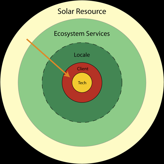
A well-designed project will make use of an integrative process, an approach that essentially dictates that the whole is greater than the sum of the parts. System design does not merely involve putting together all the required parts and constructing it into a functioning system. It involves careful consideration of how each part fits into the overall system goals set by the stakeholders (clients), while also taking account of the environmental context the system is meant to work in.
By emphasizing the integrated design approach, we identify the solar utility, client and stakeholder, and project locale as the three main components for the goal of solar design. Each of these cannot be addressed without engaging the frameworks of the other two. These components also play a vital role as constraints. Constraints are useful tools for designers since they serve as guidelines for the design decision process.
The design process starts with establishing system goals. The responsible stakeholders generally define the system goals by stating what requirements they have for the system. The solar designer must take this information, coupled with the project locale and solar utility, to determine how much energy can be produced. In the next few sections, we will go into some detail on all of these.
Failure to consider all the important aspects in the design of any project will eventually lead to a system that performs poorly.
11.3 Preparing your project proposal draft
Learning Activity: Preparing your project proposal draft
Now it's time to pull the prior work together for a proposal to your clients. You are to use both SAM and your knowledge about the solar resource and economic decision making to propose one or more solar solutions for your client.
Remember: The Goal of Solar Design is to:
- Maximize the solar utility
- For the client
- In a given locale.
Your proposal should demonstrate the full spectrum of skills that you have been developing to accomplish this goal of solar design. At the same time, the proposal should not be a heavy technical paper but rather should be crafted as a well-justified pitch to your client. The technical data on project design should be used to strengthen and support your message, not to confuse your potential reader.
In this course, the information covered has been broken down into three distinctive arcs:
- Technological Assessment: resource assessment, technology assessment, system performance simulations
- Economic Assessment: financial analysis, incentives, elasticity of demand, comparison of alternatives
- Sustainability/Risk Assessment: broader impacts, ways to reduce risk, uncertainty analysis, policy, stakeholder analysis, sustainability, and ecosystems services
The project proposal should present some data and analysis to address all three of these important aspects of project development.
Tools to use:
Use any and all available tools to form a creative project proposal that will engage your client and be a compelling first step in project development. Using SAM software will be required, and I recommend that you use the "Create/Duplicate Case" menu to explore various options for a SECS project on behalf of your client. Go back to Lesson 6 for ideas, too. You are welcome to use the financial analysis spreadsheet we worked with in Lesson 7, although that is optional - you can as well use SAM for financial modeling.
Here are some resources from the USA Dept. of Energy:
- Open EI [173]: Energy Information Database
- Buildings Performance Database [275]
- Green Power Network [276]
- Database of State Incentives for Renewable Energy [166] (DSIRE)
There are also the extensive resources available at the 7Group website [147]:
Key elements to include in your draft:
- Title /author's name / date, semester (you can include a separate title page to improve the looks)
- Introduction - brief synopsis on what this project is about, motivation, and goals
- General information on locale, client, and potential stakeholders
- Building/site characterization (if appropriate: energy demand and energy provider)
- SECS options: analysis of Solar PV /Solar Hot Water / or other and design (including efficiency strategies)
- Economic Considerations (cost analysis, incentives, payback..)
- Environmental Impacts and Ecosystems Assessment (consider both positive impacts and possible concerns)
- Recommended Integrative Design Plan (charrette, timeline, implementation, plan for commissioning and maintenance)
- References
When writing, try to look at your narrative through a stakeholder's lens. It is important to relate the analysis you do to your client's goals and clearly explain the presented information to your audience. It is good to finish your proposal with a strong statement summarizing your key findings and benefits your project would bring.
This week, at the pre-proposal stage, you may not be able to complete all of the elements and include all data you want to include. That is fine. If you need more work on a specific part of your proposal - just make space for it, provide a heading, and a description of what is to be completed and to be included in the final document, so that your reviewer sees that you do are not forgetting anything important. Also, the above list can be used as proposal structure, but if you see a need to modify it to better fit your case, please feel creative.
Deliverables this week
For the first draft (pre-proposal), develop a 5-7 page document (Doc or PDF format) that would be a hybrid of an outline and written report (you can expand on finer details later in the final submission). This work is somewhat similar to Lesson 6, but this time you are specifying your own client and locale. Please submit your pre-proposal draft and *.sam file to "Project Proposal Draft" dropbox in Canvas. Further, you will be able to see someone else’s proposal assigned to you for review in the same dropbox. The peer review assignments will be made by the instructor.
Once all pre-proposals are in, you will have several days for the peer-review task. You will need to send your peer-review and annotated author's proposal directly to the author and will submit it to a separate dropbox in Canvas for instructor's assessment. More detailed peer review instructions are given on the next page of this lesson and in Canvas. Please provide constructive feedback to your peers. You may also get new ideas for your own project from your peers during this review process, and your peer will provide you with ways to strengthen your own proposal. So, the benefits should be multifold, and if you each strive for excellence and creativity, your final proposal due in the final week will be strong and compelling and will have a high likelihood of receiving a high grade.
Please see the grading rubrics for the pre-proposal, peer-review, and final proposal tasks in Canvas.
Deadlines
Check the Canvas Calendar for specific due dates.
11.4 Reviewing your Peers' Project Proposals
Learning Activity - Peer Review
In Canvas you will be provided with access to one of the submitted pre-proposals to make your review. While you should feel creative about reviewing your peers' work, I also want to provide you with some guidelines to make sure none of the key points are missed.
Three deliverables
- Edit the submitted PDF: Your peers are responsible for producing PDF documents for you to review. You are then going to mark up the PDFs with your own comments.
- Check the *.sam file from the simulations: Your peer should share his/her SAM model with you as a source of data to review. You don't need to dig deep into it, but it will be useful to check the SAM results against the statements in the proposal draft.
- Compose a reviewer summary: Take your analysis of the draft and write up a formal review in a summary narrative (and save it as a PDF document).
You can use the following 8 criteria elements to structure your reviewer summary. Try to compose your comments in the third person, and back up your constructive criticism with examples found in the document (or the absence of content). Most reviews of compelling proposals will be 1-2 pages. If extensive errors or omissions are found, the itemized listing of corrections may extend the review length. You will be evaluated on your ability to provide constructive feedback to your peer that will strengthen their final proposal.
Peer Review should include (feel free to use these items as subheadings in your review document):
- Summary: Quick executive statement of what is presented (e.g. Jane D. has presented a proposal " <Title> " for ... that compares ... with ...)
- General comments: A broad statement of your impressions gathered in reviewing the proposal. This should include any major errors or omissions that appear to seriously weaken the proposal. This should also include constructive and positive statements of the proposal overall.
- Itemized list of corrections: A short bulleted listing of suggested corrections or errors found in the document, identified by page number. This list can also be linked to groups of errors found in the PDF for expediency.
- Innovativeness: Was this proposal creative, novel, or used non-traditional approach to the goals; or was the proposal fairly standard in its approach? This is not a good or bad interpretation of the content, rather a statement of a compelling and novel approach.
e.g. The overall approach made use of extensive research into the solar resource in a creative way by ... - Relevance to the Goal of Solar Design: Did the author appear to fulfill the goal to maximize solar utility for the client in the given locale?
e.g. The author created a compelling argument that involved a detailed analysis of the stakeholder...and formed a well-defined context for the locale... - Practical relevance: Is this proposal grounded in both financial and solar resource foundations, or might the author be over-/understating the claims for performance?
- Clarity of the manuscript: A summary statement of the spelling/grammar, organization of content, and proper use of visual imagery to sway the client
- Recommendation: This is analogous to a recommendation for publication in a peer-reviewed journal process
- proposal rewrite will need major revisions before submission,
- submit proposal rewrite with minor revisions noted in PDF,
- rewrite content as-is into the final proposal (aka: the author walks on water)
Submitting Your Work
Please upload your (i) marked-up PDF and (ii) Reviewer Summary to the "Peer Review of Project Proposal" dropbox in Canvas, and, please, also send a copy of each directly to your peer through Canvas Inbox by the assigned deadline.
Grading criteria for peer reviews
Your peer review will be evaluated out of 15 pts.
- 5 points: marked-up PDF indicates that the entire document was reviewed in detail in an attempt to strengthen the proposal. (3 pts if document appears to have been scanned only for major errors)
- 10 points: reviewer summary is complete, with all the above-listed 8 criteria elements addressed in a thoughtful manner. Full points when student establishes clear and constructive comments that attempt to strengthen the proposal for the final submission.
11.5 Summary and Final Tasks
Summary
Thank you for your great work pulling your first drafts together, and reviewing the content from your peers. By this time, you should be finding that the goal of solar design and engineering provide us with a framework to flesh out compelling proposals for future solar energy conversion systems development. You may also have noticed the benefit of working with peers to improve your approach and strengthen or focus your proposals. This is again a part of the integrative design process.
Think about the larger teams that you will need to be a part of in future projects. Is there an ideal transdisciplinary team that you might recruit to develop and deploy future solar projects?
Reminder - double check that all the deliverables for Lesson 11 are completed!
You are ready to move on to the final phase of EME 810.
See you in Lesson 12!
Lesson 12 - Solar Design Project Proposal
12.0 Overview
Overview
This lesson is the culmination of our work over the semester. You will be finishing your Solar Design project proposals on behalf of your clients in their given locale. By this time, you should have received feedback from your peers on your draft outline. This week, we will refine that document into a formal proposal for the client, synthesizing the many aspects that have made up the goal of solar design: to maximize the solar utility for the clients/stakeholders in their given locale.
Good luck with your work this week, and please take advantage of the forum or email correspondence to help to refine your design concepts. Project design does not occur in isolation!
12.1 Learning Outcomes
By the end of this lesson, you should be able to:
- compose a design project proposal that addresses the goals of solar design and engineering.
What is due for Lesson 12?
This lesson will take us one week to complete. Please refer to the Course Syllabus for specific time frames and due dates. Specific directions for the assignment below can be found in this lesson.
| Required Reading: | None |
|---|---|
| To Do: | Finish composition of your final proposals and submit your work in Canvas. Contribute to the final discussion forum. |
| Topic(s): | Goal of Solar Design, Integrative Design Team. |
Questions?
If you have any questions, please post them to the Lesson 12 General Questions and Comments Discussion Forum. I will check the forum regularly to respond. While you are in a discussion, feel free to post your own responses if you, too, are able to help out a classmate.
12.2 Discussion Activity: What is a Superior Design Team?
Yellowdig Discussion
So far, you have been working individually, or with the feedback from a peer, to design a project proposal. This proposal has elements of solar resource assessment, system engineering, financial assessment, social and policy awareness, ecosystem services - hollistically combined in a sustainable approach to energy systems. If that seems like a lot for one individual to wrap their mind around, you're right!
In our last discussion activity of the semester, I would like you to post your dream team of integrative design. Imagine that you just started a small solar design firm. You now need to hire a team to help you build your company name by reputation of being highly reliable, economically competitive, and producing high-quality solar projects.
What members would you want in your team, and what skills would they need to bring to the table?
Post your thoughts on the Yellowdig Discussion this week. Do not forget to read everyone's posts and provide your feedback too.
Tagging
We have a couple of new topics added to Yellowdig menu to facilitate discussion over the final weeks of the semester. Also, feel free to revisit any previous topics, especially if your project building research provided you with some new insights or resources you'd like to share:

Grading and Deadline
These last two weeks of the semester are your last chance to contribute to the EME 810 Yellowdig Community and boost your participation grade. Each weekly point earning period ends on Friday. You can't go back and make things up - it is a live forum! Any activity you generate contributes to the current week grade only. Maximizing your score now (max 1350 per week) does help you offset missed weeks in the total semester score. Remember Yellowdig discussions will account for 15% of your final grade.
Thank you for your active participation in the community discussions this semester!
12.3 Summary and Final Tasks
Summary
We have finally come to the conclusion of EME 810! Great work! In this semester, we focused on the major topics of project proposal development for solar energy conversion systems. We addressed engineering tasks, financial tasks, and broader social, ecological, and policy aspects in proposal development.
You have put in a lot of effort, and hopefully the study material and practical assignments in this course brought your understanding of solar energy to a new level. Congratulations!
Remember to submit your project proposal for final assessment!
Please check the proposal submission date in Canvas Calendar and your to-do list in Canvas for any outstanding tasks.