Lesson 2 - Tools for Time and Space Relationships
2.0 Overview
Overview
This is the first of three fairly intense lessons covering the fundamentals of solar energy. You will need to distill a lot of information and work hard to internalize the key topics. Make sure that you use the discussion forums to communicate with your peers, and be sure to ask questions. Most of us have learned bits and pieces of the following materials, but never together in one setting. And for some of us, this is the very first time we are learning to juggle all the balls that tie together solar energy. You can do it!
Time and Space are related! This lesson will discuss the tools needed to evaluate spatial and temporal relationships:
- of the Sun relative to the Earth;
- of the Observer on the surface of Earth relative to the Sun at any given time;
- while identifying the angles used to describe the orientation of a Solar Energy Conversion System (SECS) surface relative to the moving Sun;
- also identifying the times that local shadows might obscure our SECS. We will use sun charts to analyze shadows with respect to solar collectors.
Just like with navigation in a ship or an airplane, time and space relations are linked together in Solar Energy and can be represented and communicated as geographic information. We input that geographic information in terms of angles and use key relations from spherical trigonometry to make time and space relations easy to calculate with a computer. For our purposes:
angles = coordinates in space and time.
The tools we develop are going to explain the sun’s position relative to any point on the surface of the Earth. Once developed, our useful equations can also be applied to estimate the time and location of shadows that block SECSs or tracking technologies for SECSs.
Math warning!
You will observe substantial mathematical relations in this lesson, and you will be expected to demonstrate your skill at applying them to solar problems in shading assessment. These equations are at the core of software like SAM, and a student completing this course should be very familiar with their application. Stick with it!
2.1 Learning Outcomes
By the end of this lesson, you should be able to:
- identify and apply the Earth-Sun Angles and the relations/equations between Solar Time and Watch Time (Standard/Daylight Savings);
- identify and apply the Observer-Sun Angles and be able to create a Sun Chart for shading analysis linked with the SAM software;
- identify the Collector Angles used to describe the orientation of a collector surface relative to the moving Sun (fixed or tracking) for power output analysis linked with the SAM software;
- list the important roles of geospatial relations to the three-part goal of Solar Energy Design.
What is due for Lesson 2?
This lesson is loaded with material on Sun-Earth geometry and will take us two weeks to complete. Please refer to the Canvas Calendar for specific timeframes and due dates - those can vary from semester to semester. Specific directions for the assignments below can be found further within this lesson.
| Required Reading: |
J.R. Brownson, Solar Energy Conversion Systems (SECS), Chapter 1 - Introduction, Communication of Units and a Standard Solar Language J.R. Brownson, Solar Energy Conversion Systems (SECS), Chapter 6 - Sun-Earth Geometry J.R. Brownson, Solar Energy Conversion Systems (SECS), Chapter 7 - Applying the Angles to Shadows and Tracking W.A. Beckman, J.W. Bugler, P.I. Cooper, J.A. Duffie, R.V. Dunkle, P.E. Glaser, T. Horigome, E. D. Howe, T.A. Lawand, P.L. van der Mersch, J.K. Page, N.R. Sheridan, S.V. Szokolay, G.T. Ward (1978). Units and symbols in solar energy [2]. Solar Energy 21, 65–68. |
|---|---|
| To Do: |
Quiz (see Canvas) - due by the end of first week Yellowdig Discussion: Reflection on time conversions / Daylight savings Learning Activity: Shadow diagrams with Sun Charts - due by the end of the second week Engage in all Try-This and Self-check activities (not graded). |
| Topics: | Directionality of light: source to sink Solar Time vs. Watch Time Sun-Earth relations Sun-Observer relations Collector orientation and shading effects |
Questions?
If you have any questions, please post them to the Lesson 2 General Questions and Comments Discussion Forum in Yellowdig. I will check these forums regularly to respond. Feel free to go through the comments and post your own responses if you are able to help out a classmate.
2.2 Basic Solar Jargon for Energy and Power
Reading Assignment
We start by reviewing these small sections on language. There are things to measure and symbols for those metrics that we need to agree upon throughout the class.
- SECS, Chapter 1, Introduction. Please pay particular attention to the final section: "Communication of Units and a Standard Solar Language." You may also download the original paper from Canvas ("Beckman_etal_1978.pdf").
While reading, consider the following points:
- What is the difference between power and energy?
- What is the difference between power density and energy density?
- What is irradiance? What is the symbol for solar irradiance?
- What is irradiation? What are the symbols for irradiation on hourly and daily steps?
- Think about the angles that we use to describe spatial and time relationships in solar energy.
-
Units and symbols in solar energy [2] (Beckman et al., 1978). You can also access this article through Penn State's Electronic Course Reserves.
Solar Energy Journal [3] was established for the International Solar Energy Society (ISES) [4] and has been around for some time now. Solar Energy Journal stands as an important forum for peer to peer sharing of solar research for energy conversion and human applications of solar energy. What I want to establish here is that there is precedent for the complex system of notation used in the solar energy world that has been in use for decades. The original authors have established the following observations:
"Many disciplines are contributing to the literature on solar energy with the result that variations in definitions, symbols and units are appearing for the same terms. These conflicts cause difficulties in understanding which may be reduced by a systematic approach such as is attempted in this paper.
It is recognized that any list of preferred symbols and units will not be permanent nor can it be made mandatory, as new terms will emerge and old ones become less used with the development of the subject. But in the meantime, a list would be appreciated by the many workers who are entering this multi-disciplined field...
...Energy: The S.I. (Systèm International d'Unités) unit is the joule ( ). The calorie and derivatives, such as the langley (cal cm-2), are not acceptable.
No distinction between the different forms of energy is made in the S.I. system so that mechanical, electrical and heat energy are all measured in joules. However, the watt-hour (Wh) will be used in many countries for commercial metering of electrical energy...
Power: The S.I. unit is the watt ( ). The watt will be used to measure power or energy-rate for all forms of energy and should be used wherever instantaneous values of energy flow are involved. Thus, energy flux density will be expressed as W/m2 or specific thermal conductance as . Energy-rate should not be expressed as $J/h$.
When energy-rate is integrated for a time period, the result is energy which should be expressed in joules, e.g. an energy-rate of 1.2kW would if maintained for one hour produce 4.3 MJ."
W. A. Beckman, et al.
| It is preferable to say | Rather Than |
|---|---|
In summary: received energy flux density (or power density, called irradiance) can be expressed in units of W/m2. We also note that the received radiative energy density (called irradiation) can be expressed in units of J/m2, or in units of Wh/m2. Notice that we did not use radiation, which is an expression of light glowing outward (emitted light, different direction than what we want).
In today's maps of the solar resource, you will often see the units expressed in kWh/m2. You should be aware that these are still only representations of solar light energy density, and not the hourly/daily/annual quantity of potential electricity that could be produced. To find that value, we need a simulation tool like SAM (System Advisor Model, which you should have downloaded at the end of Lesson 1), which takes irradiation data and converts it into power data.
I would like you to now take a short self-quiz to see if you recall the common uses of the notation and descriptions for solar energy (used in particular in this class.).
Self-Check
2.3 Basic Solar Jargon for Angular Relations
When we want a shorthand to describe spatial relationships on continuous surfaces that are sphere-like, as with the Earth and the surrounding sky and stars, we choose to use Greek letters. In contrast, when we are trying to communicate things like linear distances, lengths, time, or simple Cartesian coordinates, then we will tend to use Roman letters for our shorthand.
You may notice in your reading of older textbooks that several systems of sign convention for the angles have emerged for practical use. Also, the various systems can have different approaches to azimuth that we should be aware of. For instance, the software SAM (System Advisor Model) will use both the $360^\circ$ clockwise standard (from Meteorology) as well as the $\pm180^\circ$ standard used extensively in the component-based models of TRNSYS and SAM. We will be sure to become familiar with both.
Below are four tables showing the Angular Symbols for Standard Solar Relations.
General Angles
| Angular Measure | Symbol | Range and Sign Convention |
|---|---|---|
| altitude angle | (alpha) | 0o to + 90o; horizontal is zero |
| azimuth angle | (gamma) | 0o to + 360o; clockwise from North origin |
| azimuth (alternate) | (gamma) | 0o to ±180o; zero (origin) faces the equator, East is + ive, West is - ive |
Earth-Sun Angles
| Angular Measure | Symbol | Range and Sign Convention |
|---|---|---|
| latitude | (phi) | 0o to ± 90o; Northern Hemisphere is +ive |
| longitude | (lambda) | 0o to ± 180o; Prime Meridian is zero, West is -ive |
| declination | (delta) | 0o to ± 23.45o; Northern Hemisphere is +ive |
| hour angle | (omega) | 0o to ± 180o; solar noon is zero, afternoon is +ive, morning is -ive |
Sun-Observer Angles
| Angular Measure | Symbol | Range and Sign Convention |
|---|---|---|
| solar altitude angle (complement) | (alphas is the complement of thetaz) |
0o to + 90o |
| solar azimuth angle | (gammas) |
0o to + 360o; clockwise from North origin |
| zenith angle | (thetaz) |
0o to + 90o; vertical is zero |
Collector-Sun Angles
| Angular Measure | Symbol | Range and Sign Convention |
|---|---|---|
| surface altitude angle | (alpha) | 0o to + 90o |
| slope or tilt (of collector surface) | (beta) | 0o to ±90o; facing equator is +ive |
| surface azimuth angle | (gamma) | 0o to + 360o; clockwise from North origin |
| angle of incidence | (theta) | 0o to + 90o |
| glancing angle (complement) | (alpha) |
0o to + 90o |
2.4 Earth's Tilted Axis and the Seasons
Reading Assignment
- SECS, Chapter 6: Sun Earth Geometry (scan through the entire chapter first.)
Please scan all of Chapter 6 right away, to get an initial overview of the role of angles and time together with the relative positions of the Sun, Earth, and the SECS that your client would like to install. We use several angles throughout this chapter (check back to the Table of Angular Symbols [5] anytime, also found in the textbook Ch. 1). We also use a whole lot of dense equations. Don't be intimidated by the equations; they are all based on the trigonometry for a spherical surface, and we will break them down in chunks in this lesson. Just take note of them and keep reading. Take a few notes in the margins as you go!
In this first assignment, we are going to get familiar with the angular relations between the Earth and the Sun, and the relation of those angles to things like Seasons! You are all familiar with the concept that winters are cold, and summers are hot, but why??
Keep an eye out for the cosine projection effect. This is something that we often wish to minimize by tilting our solar energy conversion systems up toward the predominant diurnal (daily) arc of the Sun averaged over the year.
Earth's Rotation
As we have seen in our reading, the Earth rotates with a roughly constant speed, so that every hour the direct beam (a ray pointing from the surface of the Sun to a spot on Earth) will traverse across a single standard meridian (standard meridians are spaced 15° apart). The implications are that the unit of one hour is equivalent to the rotation of Earth 15 degrees. When Earth rotates such that the beam of the sun shifts +1° of longitude from East to West: it takes 4 minutes of time.
- 1 h = +15° Earth rotation
- 4 min = +1° Earth rotation
Wild fact: a time zone change of one hour is really just 15 degrees of separation between standard meridians.
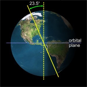
The axis of rotation of the Earth is tilted at an angle of 23.5 degrees away from vertical, perpendicular to the plane of our planet's orbit around the sun.
The tilt of the earth's axis is important, in that it governs the warming strength of the Sun's energy. The tilt of the surface of the Earth causes light to be spread across a greater area of land, called the cosine projection effect.
Cosine Projection Effect
When you tilt a surface away from a beam of light, you spread the same density of light across a larger area. Recall that irradiance is in units of W/m2, so a larger denominator means a smaller value of irradiance, right?
Explore the concept of the cosine projection effect in the following experiment.
Self-Check
This links directly with Chapter 6: Experiment with a Laser of SECS.
Watch the video of the virtual flashlight below and then answer the questions.
Video: Light intensity experiment using a flashlight (0:17)
In this video, changes made to the angle of the flashlight affect light intensity. The shallower the angle, the more the light spreads out, resulting in a lower intensity.
Seasons and the Cosine Projection Effect
The sun is about 93 million miles away from the Earth (equivalent to ~150 million km). That is so far away that the photons from solar irradiation effectively travels in parallel rays. So, unlike the flashlight experiment, the tilt of the sun has no bearing on the intensity of the radiation reaching the Earth's surface. Instead, we find that the Earth's tilt controls the intensity of irradiation and the seasons.
Keep in mind that the Earth's axis points to the same position in space (toward the North Star, Polaris). As the Earth travels in a near spherical (a very small eccentricity into an ellipse) orbit around the sun, the Northern Hemisphere can be tilted toward or away from the sun, depending on its orbital position.
SPRING: (Image of the tilt of the earth in the spring) In this configuration, the earth is not tilted with respect to the sun’s rays (The earth in this picture is actually tilted towards you as indicated by the fact that you can see the North Pole – green dot). Therefore, radiation strikes similar latitudes at the same angle in both hemispheres. The result is that the radiation per unity area is the same in both hemispheres. Since this situation occurs after winter in N. Hemisphere we call it spring, while in the S. Hemisphere it is autumn. This occurs on March 21.
SUMMER: (Image of the tilt of the earth in the summer) When the N. Hemisphere is tilted towards the sun, the sun’s rays strike the earth at a steeper angle compared to a similar latitude in the S. Hemisphere. As a result, the radiation is distributed over an area which is less in the N. Hemisphere than in the S. Hemisphere (as indicated by the red line). This means that there is more radiation per unity area to be absorbed. Thus, there is summer in the N. Hemisphere and winter in the S. Hemisphere. This situation reaches a maximum on June 21.
AUTUMN: (Image of the tilt of the earth in the autumn) In this configuration the earth is not tilted with respect to the sun’s rays (The earth in this picture is actually tilted towards you as indicated by the fact that you can see the North Pole – green dot). Therefore, radiation strikes similar latitudes at the same angle in both hemispheres. The result is that the radiation per unit area is the same in both hemispheres. Since this situation occurs after summer in the N. Hemisphere we call it autumn, while in the S. Hemisphere it is spring. This occurs on September 21.
WINTER: (Image of the tilt of the earth in the winter) When the N. Hemisphere is tilted away from the sun, the sun’s rays strike the earth at a shallower angle compared to a similar latitude in the S. Hemisphere. As a result, the radiation is distributed over an area which is greater in the N. Hemisphere than in the S. Hemisphere (as indicated by the red line). This means that there is less radiation per unit area to be absorbed. Thus, there is winter in the N. Hemisphere and summer in the S. Hemisphere. This situation reaches a maximum on December 21.
Self-Check
Click on "Summer" in the above animation. When the Northern Hemisphere tilts toward the sun, the irradiation has a lower angle of incidence, meaning more photons strike a smaller area during the daytime. Answer the following questions for yourself. If you have any questions, please post to the Lesson 2 Discussion Forum.
- What happens to the Southern Hemisphere?
- What is the correlation with concentrated sunlight and the seasons?
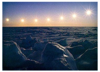
- What happens beyond the Arctic Circle, which spans from about 66.5 degrees latitude to the North Pole?
Now, answer the same questions for autumn, spring, and winter.
Forecasters and meteorologists use different criteria to determine the "meteorological seasons." For example, meteorological winter in PA runs from December 1 to Feb 28/29, a period that statistically includes the three coldest months of the year. This is also centered on a time about 25 days after the Winter Solstice.
Meteorological summer runs from June 1 to August 31, a period that includes the warmest three months of the year. Again, this is a period centered about 25 days from the Summer Solstice.
As one more example, review Pittsburgh's plot of annual average high temperatures. The maximum daily temperature occurs in late July, long after the summer solstice.
Self-Check
2.5 Solar Time and Watch Time
Reading Assignment
- SECS, Chapter 6: Sections titled "Time Conversions"
In this continued reading of Chapter 6, you will be focusing on the way that we account for time in solar energy and the relation of time to more spherical angles. We will use those angles to later calculate the estimated irradiance and irradiation conditions just outside of the Earth's atmosphere (called Air Mass Zero: AM0).
Pay attention to the use of solar time vs. watch time (which will be expressed as standard time vs. daylight savings time). In solar simulation tools like SAM (System Advisor Model), we will only be using solar time, which is the industry norm. Watch time is just a convenient way to get everyone to work at the same time, and to coordinate conference calls. Your job is to get out of watch time and into thinking in terms of solar time, and the angles those times represent.
As we see in the reading, time is a critical parameter in solar energy resource assessment, and we use a "different" time from your mobile phone (or if you have one, a watch). The time that we use in solar energy is the apparent time and path of the sun relative to the aperture or collection device, called Solar Time.
- A solar day is 24 hours long, and Solar noon is always used locally as the center of time.
- Solar noon is defined as the moment when the Sun is at its highest point in the sky.
- The hour angle for solar noon is (given the symbol of lowercase omega).
- Time before solar noon counts backward from , and so the angles are negative.
- Time after solar noon counts forward from , and so the angles are positive.
Correcting Time for Big Longitude Changes: Standard Meridians
The time that you are used to using on your laptops, phones, and (if you still have them) watches is called Standard Time, and is referenced back to the Coordinated Universal Time (UTC), the primary time standard by which the world regulates clocks and time.
Our notion of time is also tightly coupled with our system of longitude (the longitude symbol for us is ). We have used lines of longitude, or meridians, as a reference for time and position E-W. Because time and angles are all linked together, we cannot escape the sexagesimal (base 60 math) system for geographical locations. As we demonstrated earlier in the lesson, each standard meridian (a major line of longitude) is spaced 15° apart, beginning with the Prime Meridian () in Greenwich, England, and continuing for 360 degrees, or 24 hours.
I live someplace other than Greenwich. How do I account for Longitude ()?
Your standard time zone will tell you the standard meridian (). For example, the EST is -5h from UTC, while Central European Time (CET, like Paris) is +1h from UTC.
- For every standard meridian shift to the West, you will need to subtract 15 degrees per hour.
- For every standard meridian shift to the East of the Prime Meridian, you will need to add 15 degrees per hour.
Self-Check
Answer the following questions for yourself. If you have any questions, please post them to the lesson 2 discussion forum.
- Find the meaning of UTC and solar time in Wikipedia.
- Find the acronyms for Standard Time and Daylight Savings time, each in your own time zone today. See timeanddate.com [8] for some help.
- Find the number of hours shift from UTC in your own time zone today.
- How many degrees is the Prime Meridian from your Standard Meridian, and is it the same (or less/more) than the number of hours of longitudinal shift you would expect from the reading?
- Are you in Daylight Savings time now? Would that affect the time correction?
Correcting for Little Longitude Changes: Inside Time Zones
Where you live, or where your future solar site assessment will occur, will likely be well within the edge of a time zone (meaning ). We already learned that every 1° of angular rotation on Earth is equal to 4 minutes of time. Standing in one spot on the surface, this means 4 minutes of relative time correction locally per degree of deviation from a Standard Meridian ( ). So, locales will have a local longitudinal refinement to account for, in order to account for not living directly on a 15-degree incremental Standard Meridian on Earth.
Standard Meridians define the beginning of a time zone, and not the end of a time zone. So, you are always going to look to the start of a time zone to find the Standard Meridian.
There are a few other cities that actually are well seated for solar time zone correction (close enough for our calculations):
- Philadelphia is fairly close to the EST standard meridian of -75°.
- Denver is fairly close to the MST standard meridian of -105°.
My client lives someplace other than a Standard Meridian, how do I account for that?
First, go to Google and type "<insert city name> longitude". You should get a quick response of both the Longitude (lambda) and the latitude (our symbol for latitude is lowercase Greek "phi": phi), represented in decimal form (more useful to us for trigonometry and angles).
Have you noticed that real time zones are more often political boundaries that zigzag around, rather than following an actual Standard Meridian? So, actually, there can be locales for clients that are East of their own time zone Standard Meridian, instead of the normal relative locations West of the time zone Standard Meridian. This is why, in the reading, you will see minutes per degree of local longitudinal shift away from the time zone's Standard Meridian.
Correcting with the Equation of Time: Accounting for Wobbles
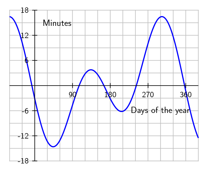
Even in Greenwich, where no longitudinal correction is necessary, "noon" UTC will generally not be the time when the sun is directly overhead. We can see in the plot below that watch time and solar time are the same in Greenwich for only 4 days in the year.
- There are deviations of up to minutes (regardless of your location on the planet).
As you will have read, our interpretation of watch time assumes an even progression for Earth's planetary rotation, with no weebles or wobbles or precession of the polar axis. However, you will now know that wobbling occurs, and there is great variability in the rotation of the earth throughout the months of the year. This is why we add leap years and leap seconds to our calendars. So, we create a "mean time" based on the length of an average day to keep things simple. Solar time has to correct for this mean time approximation. Equation of time correction versus day of the year is shown in Figure 2.7. As an exercise, you can try to calculate these curves based on the empirical equations (6.10) and (6.11) in Brownson textbook.
The following picture was a composite of images, taken at the same watch time every few days for an entire year, to record the position of the sun. We call the shape an analemma. Notice how there is a big loop and a little loop, and compare the same big waves and little waves in the first image of the Equation of Time correction above. If you were to draw a line down the center, you would have removed the error from watch time, and you would be one step closer to solar time.
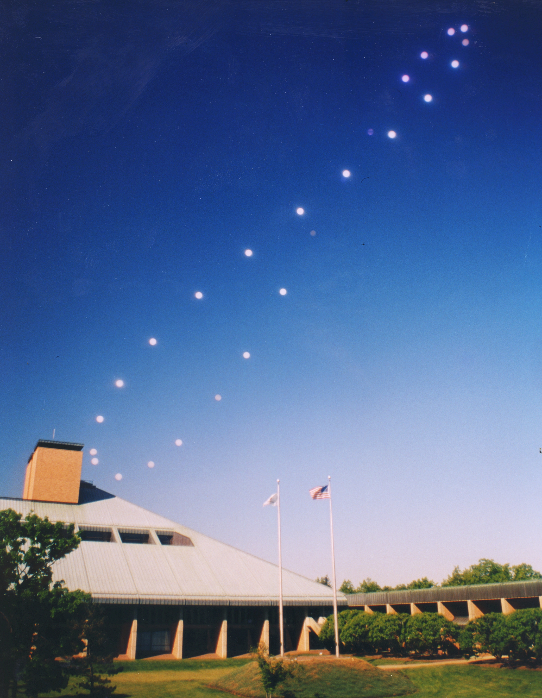
For views of amazing solar analemma photography by Anthony Ayiomamitis, also, please visit the Stanford SOLAR Center [11].
These images were taken at the same time and location every day for one year. You will see the curve described by the Sun over that year. An analemma is a beautiful way to capture both the range of declination $\delta$ (along the length of the analemma) and the Equation of Time Et (the expansion or width of the analemma) in a graphical format.
Putting Time Correction Together:
As we have seen in the reading, we have a method to correct local watch time to solar time, to correct for the true time of day according to the sun relative to the meantime.
The time correction factor is a function of the equation of time, the meridian of the local standard time zone (Lst), and the longitude of the collector/observer (Lloc), and the Equation of Time (Et). The equation of time correction accounts for the wobble and is the first step. Then we need to correct for the change in longitude leading to time zones (standard meridians occur every 15 degrees) and the change of time for locales that are not located along standard meridians.
In these conversions, each year is assumed to begin just after midnight, Dec. 31, and time counts up from there. The time corrections here are in terms of minutes, not hours. The Equation of Time corrects the time to mean solar time (by adding or subtracting up to 16 minutes of correction). The Time Correction Factor corrects time for your shift in Latitude from each Standard Meridian (which occurs every 15 degrees away from the Prime Meridian). Daylight Savings Time is an optional correction, as there is a +60 minute difference from Standard Time between March and November in the USA (and some other regions of the world).
2.6 Let's Convert Solar Time to an Angle
Reading Assignment
- SECS, Chapter 6: Review both sections of "Moments, Hours, and Days" as well as Sun-Observer Angles."
In reviewing these sections, you should notice that three common angular symbols keep popping up: the declination (), the local latitude (), and the hour angle (). As we shall again see in the next section, these are three of our key Earth-Sun angles.
We additionally include the use of longitude () in our calculation of time, and in particular, converting time to an angle: the hour angle.
Now, let's convert "time" into an angle, for our future trigonometric relations:
When we convert time to an angular value, we can no longer use a 24 hr format. We need to convert hourly time into a useful angle based on the properties of a sphere, again using spherical trigonometry.
Video: Hour Angles (5:03)
So, I'm sure a lot of you are wondering what we do with the hour angle. Because it's not something that we really ever used before in regular everyday language. But because so many of our mathematical calculations are in terms of angles, remember, angles are coordinates in the solar reference in the solar frame of reference.
So, when we normally have 24-hour time, we need to convert that time into something on the order of 360 degrees or, in our case, minus 180 degrees to plus 180 degrees. And so, we're going to figure out a way to convert 24 hours of time to degrees. And those degrees are going to be found as the hour angle.
So, time is going to be in terms of decimal hours. So time in decimal hours. And we're going to make sure that we do that in a 24-hour time frame, so that if I were talking about 1:30 in the morning, I would represent this as 1.5. If I wanted 1:30 in the afternoon, based on the 24-hour system, that would be 13.5. So we have that understood.
So, in order to get the hour angle of time, we're going to start with time is going to be the hour angle times the conversion of one hour per 15 degrees of rotation of the earth. So that's going to give me my decimal hours-- multiplying right there-- such that if I wanted to have the hour angle, I would have time times 15 degrees per one hour. In which case, my time is in hours. The units of hours would cancel out. And I'd be left with units of degrees.
Now, one of the things that you're going to find in your problems is the calculation of day length. And if the day length in the textbook is shown by calculating the hour angle of the sunset-- and we do sunset because it's a positive angular value. Basically, if I were to-- here, let me do a quick diagram.
If I were to put noon, 12:00 noon here, any time before noon would be negative. Any time after noon would be positive. So, this is where I have my negative 180 degrees going into the morning. You're looking back before noon, so you have negative degrees. Going into the afternoon, you're going after 12. So, you're adding degrees. So it's positive.
So, I have a positive value for the sunset. So, if I wanted to calculate the sunset, we find that I need to calculate the arc cosine or the inverse cosine of the negative tangent of the declination times the tangent of the latitude, phi. And I might have switched these two guys around in the textbook. But you're going to get the same answer.
So, that will give me the time of sunset or the hour angle of sunset. And the hour angle of sunrise is going to be the negative of the sunset. And then the last part that you're looking for, hours in a day, is going to be 2 times the sunset hour angle times the conversion of one hour for 15 degrees. That's going to give you the number of hours in the day. And you're going to want that for one of your answers as well.
Finishing Step for Time Conversions! The Hour Angle () in decimal degrees.
We represent the apparent displacement of the sun away from solar noon, either as a negative or positive angle. An of zero indicates that the sun is at its highest point for that given day.
- The sign of the hour angle before noon is negative, because we have to count backward from the "zero hour" of solar noon.
- The sign of the hour angle after noon is positive, because we are counting forward from the "zero hour" of solar noon.
Another way of looking at it is the angular difference between the local meridian of the observer/collector and the meridian that the beam of the sun is intersecting at a given moment.
Now, the day won't really begin at -180 degrees, anywhere between the arctic circles. However, I wanted to emphasize that the day only begins at -90° on two days a year. Those days occur during the Equinox moments in the orbit of the Earth about the Sun, and the length of those days is actually 12 hours long. All other days are either shorter than 12 hours, or longer than 12 hours. As such, they end either less than 90° or greater than 90°.
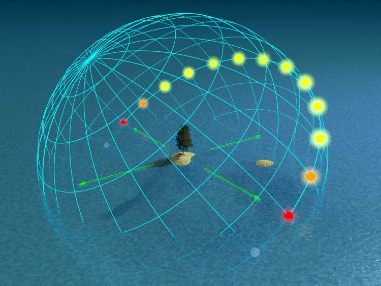
The images below demonstrate singular arcs of the Sun for each hour in solar time, at five different latitudes on Earth (no analemma correction necessary). The peak hour (or the hour with the highest solar altitude angle) is defined as solar noon. You will notice that the solar equinox has twelve sun spots for latitudes below the arctic circle, and that the sun rises due East, while setting due West. During the solar solstices, you see multiple arcs: one for winter and one for summer. Notice that there are more hours of the day in the summer, and the sun rises farther from the equator in the Summer (sun rise in the northeast for the Northern Hemisphere).
What else do you notice in comparing the four critical times of year at different latitudes?
Solar Equinox
 [14]
[14]  [15]
[15]  [16]
[16]  [17]
[17]  [18]
[18]
Solar Solstice
 [19]
[19]  [20]
[20]  [21]
[21]  [22]
[22]  [23]
[23]
Now, we are ready to use hour angle to find out positions in our solar design projects!
Self-Check
2.7 Let's Convert Time from Watch to Solar
Remember that the Earth rotates at 15 degrees per hour, and 0.25 degrees per minute. It can get confusing when you're comparing spatial seconds with temporal seconds, right? That's why we will stick with decimal notation in all of our references to latitude ($\phi$), longitude ( ), and angles (degrees).
Self-Check
Step 1: Correcting for Standard Time (Standard Meridian) in Hours: Find the time zone of your client. The hourly longitude correction is plus or minus X hours from the Prime Meridian, where UTC = 0h. Multiply the positive or negative hour value by 15°, and you will know your standard meridian for the Time Zone.
Key: Your standard meridian for your time zone begins on the East side of the time zone. (Sun rises in the East, right?)
Step 2: Correcting for Time from the Local Longitude Relative to Standard Meridian in Minutes:
You need to know the longitude for the standard meridian of the client ( ) from their local time zone, and the local longitude of the client's location in question (). We calculate the longitudinal correction, from these two.
Keep in mind: Time zone borders are political boundaries, and can be constructed on both sides of a Standard Meridian. A locale to the east of the Standard Meridian would still be input as a positive value (the resulting minutes would be positive).
Note: we use the sign convention that longitudes are positive valued for to the East of the Prime Meridian, and negative valued to the West of the Prime Meridian. This equation is valid for both sides of the Prime Meridian. The exterior negative sign is there to make the time correction algorithm work correctly.
Step 3: Calculating Equation of Time (Analemma) Correction in Minutes (Et): We begin with the two simple coefficients of n (the day of the year, from 1-365), and B (see the first equation). Our assumption is that the year begins at midnight of the new year, and the trigonometric portions of the equation of time will take an argument of "B" in degrees.
You have seen that the Equation of Time has a graphical representation, the analemma. Once we determine a correction in the scale of minutes, we can use it in the Time Correction Factor, TC.
Step 4: Completing the Time Correction Factor ($TC$): The time correction factor is a time shift in minutes.
Recall that 0.25° of longitudinal rotation (of the planet) will consume 1 minute of time. That would make each degree of change equivalent to four minutes. Hence, we need to multiply our longitudinal correction by a factor of four to yield a consistent unit of minutes in time. This is shown as the value of the longitudinal correction (Lc) in units of minutes (temporal, not geospatial).
Step 5: Accounting for Daylight Savings Time (DST) in 60 minutes.
The equations do not tell you when DST occurs from country to country. There is a +60 minute difference between March and November in the USA. So, if we had to correct for DST, then we would need to subtract that 60 minute addition back out.
Again, make sure that the data is presented in minutes, rather than hours.
Self-Check
2.8 Discussion Activity
Continuing Conversations in Yellowdig!
I hope you are getting the hang of Yellowdig conversation platform and are ready to pick up the pace! You can access the discussion platform through the Canvas menu.
Lesson 2 Discussion: Reflection on Time Conversions
For this week, I would like you to question why we do all of these time conversions for solar energy. Why do we need to know these time and angle relations as solar energy specialists? There are many terms and concepts to reflect on – some are well-known, and some may be new to you. In this discussion you will have a chance to reflect on the meaning and your understanding of those and perhaps some of your peers’ interpretations of those concepts will be helpful to your comprehension of this lesson. Here are some guiding questions you may use as starting points for your posts:
- What is the difference between Solar time vs. Clock time? Is that important, significant, and should we bother?
- Analemma, what is it representing, and how it affects the solar time?
- What is longitudinal time correction?
- Daylight savings - what insight have you gained about the use of daylight savings in society? Is it useful, not so much, meh?
- What are equinox and solstice's role in solar resource forecasting? These are key, critical points in time. What makes them special?
This is an open-ended discussion, and you may ask questions or raise your concerns with things that might still remain confusing. Feel free to post and comment on any of the above-listed topics and whatever you want to share after working through the lesson material.
Tagging
Yellowdig Tip: When you create a post in the Yellowdig discussion space, you are required to choose a topic tag. For Lesson 2 discussions, use any of the following:
Know that you can tag your post with one or several of these topics depending on its content. It gives you flexibility to discuss these things cumulatively or, if you prefer, to break your writing into several smaller posts.
Importance of interaction
Once again: the more you participate, the more opportunities for your discussion score to grow through the week. Comment, ask questions, react, throw in additional thoughts – it all is in your benefit!
Grading
Yellowdig points you earn over the weekly point earning period (from Saturday to next Friday) will count towards 1000 pts. weekly target. But you can go above it (to 1350 pts. max) if you are feeling active. That may help you to make up for some low-activity weeks. Yellowdig discussions will account for 15% of the total grade in the course. Check back the Orientation Yellowdig page in Canvas for more details on the points earning rules.
Deadline
There is no hard deadline for participating in these discussions, but I encourage you to create your posts in the middle of the study week (Sunday) to allow others to engage and respond while we are learning specific topics in the lesson.
2.9 Sun-Earth Relations
Reading Assignment
- SECS, Chapter 6: Earth-Sun Angles section
The following sections are closely coupled to the reading assignment, but I have enlarged the images for you. Our Solar Energy Conversion Systems are going to be fixed at some location on the surface of Earth, right? So, we will place an "Observer" at the future location and describe the relative position of the Sun and Earth and SECS. However, there are a few underlying spherical relations that do not depend on the location of the SECS or the observer.
This section discusses those geometric relations that are effectively "Independent of the Observer." Keep an eye out for the declination (delta, ), the latitude and longitude ( and ), and , the hour angle.
The Greek notation used below is now fairly standard for the field, but you may see different approaches in informal settings or unusual textbooks. I follow the established nomenclature defined by Beckman, et al., in the research journal Solar Energy in 1978, reprinted in Solar Energy in 1997. As noted earlier, the document is available to you from the Library E-Reserves.
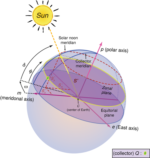
Hour Angle ():
Again, this is the way we represent the apparent displacement of the sun away from solar noon. An hour angle of zero degrees indicates that the sun is directly above, and the sign of the hour angle is determined by occurring either before noon (negative) or after noon (positive). Another way of looking at it is the difference in angle between the local meridian of the observer/collector and the meridian that the beam of the sun is intersecting at a given moment.
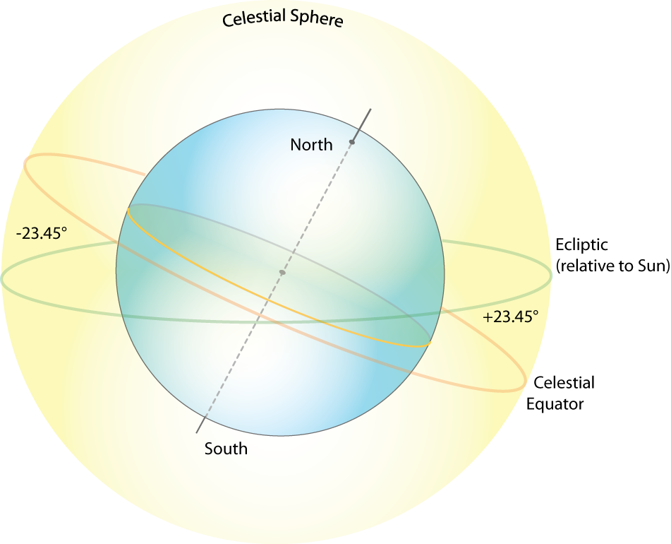
Angle of Declination ()
This is not an observed angle relative to the surface of the Earth and the Collector. Declination is the observed angle (due to the polar tilt) between the plane of the Earth’s equator and the plane of the ecliptic (the plane in which the Earth's orbit about the Sun lies). Declination has a maximum angle of 23.45° at either solstice. In this case of coordinates, the sun observed in the North is positive, and in the South is negative. One can imagine this as a series of sun paths over the course of a year. In contrast, the declination reaches a midpoint at either of the equinoxes. The range of declination is limited to Earth’s tilt: −23.45° (winter solstice) (summer solstice).
Declination is independent of location on the planet!
The declination can be calculated by a simple approximation (first equation) or a Fourier series (second equation).
where:
Angle of Latitude () and Longitude ()
The complement of longitude () in geospatial coordinates is the latitude. When combined together, we have identified a singular point on the surface of Earth. However, separately, they refer to arcs or circles spanning huge distances. We can look up the latitude and longitude of a site on a search engine like Google.
Key latitude angles of interest are:
- Arctic Circle = +66.56° North of this, the sun is above/below the horizon for 24 continuous hours at least once per year (during the solstices).
- Tropic of Cancer = +23.45° The maximum tilt of the North Pole to the Sun.
- Equator = 0°
- Tropic of Capricorn = −23.45° The maximum tilt of the South Pole to the Sun.
- Antarctic Circle = −66.56° South of this, the sun is above/below the horizon for 24 continuous hours at least once per year (during the solstices).
2.10 Sun-Observer Relations
Reading Assignment
- SECS, Chapter 6, Sun-Observer Angles section
Once we have identified our specific location on the surface of Earth, we use the spherical relations between the Sun and the fixed observer at the locale to describe the relative motion of the Sun during the day and over the year. Once again, this text is closely complementing the text in the book.
Pay attention to the fact that this particular set of relations is only for the special case of a horizontal surface. We are only describing angles for an imaginary flat surface on Earth, like a table top. In real SECSs, we will often tilt the receiving surface up (tilt has a symbol of ), specifically to minimize the cosine projection effect that occurs at a given latitude. Bear in mind that the angles for a non-horizontal surface (tilted, with some accompanying azimuth orientation ), or for a tracking system, are an entirely different set of general equations.
Also, as these relations refer to the apparent motion of the Sun, they have the subscript of "s" for the two coordinate angles of solar altitude angle and solar azimuth. The complement of the solar altitude is the zenith angle, which has a special subscript of "z".
The Solar Altitude () measures the angle between the central ray from the Sun (beam radiation), and a horizontal plane containing the observer. Note that the subscript "$_s$'' is there to indicate that the altitude relative to the observer of the Sun. This will become important in evaluating the altitude angles of other objects projected onto the sky dome, like buildings, overhangs, wing walls, and arrays of solar receivers.
The Zenith Angle () is the geometric complement of the solar altitude angle. We direct your attention to the use of here, as the general concept of the angular deviation of the Sun's ray from the normal projection of a surface is called the angle of incidence, . In effect, the zenith angle represents the angle of incidence for a horizontal surface.
Recall: "normal" means perpendicular to a surface.
The Solar Azimuth () measures the angle on the horizontal plane between the meridian of the 0 degrees axis (South, for the Northern Hemisphere, opposite Down Under) and the meridional projection of the Sun's central beam (the Sun's meridian). The convention we will use is also used in the advanced design tools for solar energy, TRNSYS (UW-Madison: Transient eNergy Simulation Software), PVSyst, and SAM (NREL: System Advisor Model). The angle varies from 0 degrees at the South-pointing coordinate axis to degrees. East (earlier than noon) is negative and west (later than noon) is positive in this basis. This is a well-used standard taken from the original text of M. Iqbal.\cite{iqbal83}
Note: the function "sign()" is specifically defined as a cases form of positive and negative notation (meaning there are two alternate cases to choose from).
There are several texts and software available that use a solar azimuth, measuring clockwise on the horizontal plane from a North-pointing (0 degrees) coordinate axis. This is also the convention for the field of meteorology and for the wind industry. This azimuth convention uses 360 degrees for the meridional projection of the Sun's central beam.
However, the majority of professional software does not use this convention yet, so you must be aware of the difference, as the math changes with the two methods. It is relevant to be aware of the difference, in that the North basis is used in the basic educations tools for simulation called PVWATTs, for the sun path tool at the University of Oregon, and in the interactive software PVEducation.org [25].
2.11 Collector Orientation
Reading Assignment
- SECS, Chapter 6: paying attention to sections of "Collector-Sun Angles" and "A Comment on Optimal Tilt"
Once we have identified our specific location on the surface of Earth, and used those coordinates to identify the location of the Sun in the skydome relative to a fixed observer in a given locale, we can enter the angles for the orientation of our SECS. Again, this text closely complements the text in the book.
What is different here?
This new set of relations is for the general cases of any surface (horizontal or tilted, fixed or tracking). We are now describing angles for real oriented surfaces on Earth, like tilted PV panels and walls of a building. As we noted in the last section, for real SECSs, the receiving surface is tilted (beta, , with an azimuth orientation γ) to minimize the cosine projection effect that occurs at a given latitude.
Also, pay particular attention to the angle of incidence (theta with no subscript, ). As part of a solar energy design team, one of our primary mechanisms to increase the solar utility for the client in a given locale is to minimize the angle of incidence at a given time during the year or day. This is an extension or refinement of reducing the cosine projection effect.
Finally, I will give you a heads-up for the next page: after reviewing these sections and completing this page, you will need to take the Lesson 2 Quiz. Note that this is a quiz with calculations, and you will likely want to have a numerical software open to work through the numerical problems.
The following angles describe the orientation of the collector surface and the relation of the collector surface to the Sun. As these three angles describe our primary surface of interest, the SECS, they do not have a subscript for the two coordinate angles of collector tilt and collector azimuth.
- Tilt: the angle between the plane of the collector (or aperture) and the horizontal. Denoted by the symbol beta, β.
- Azimuth: the planar rotation East or West that an aperture will have. Denoted by the symbol gamma with no subscript, .
- Angle of Incidence: the angle between the vector perpendicular to the collector plane, called the normal of the plane, and the projection of the Sun’s central beam to the collector surface. Denoted as theta with no subscript ().
For general cases, where the collector has a non-horizontal orientation (), the angle of incidence is not the same as the zenith angle (θz). In fact, the zenith angle is a special case of an angle of incidence for horizontal surfaces, where the zenith is referenced to the aperture as a normal projection.
The first and second angles of tilt and surface azimuth (and γ) are typically known for fixed surfaces. The third key angle is the angle of incidence (θ), which uses the following rather lengthy equation:
In order to generate an actual value for theta, we will need to also take the arccosine of the long equation. For your calculators and math programs, all of the arguments are in terms of degrees, not radians. You will need to convert degrees to radians in most programs.
However, this is a really long equation that can actually be broken down into parts. We will break up the equation for the angle of incidence (theta, ) into three lines. Take a look at them, and look for common arguments to the sine and cosine functions.
- ( , , : latitude, declination, and tilt)
- ( , , , : latitude, declination, tilt, and then collector azimuth)
- ( , , , , : latitude, declination, tilt, collector azimuth, and then the hour angle)
Mechanisms to Maximize Solar Utility:
In the introduction of the textbook, there is a reference to the goal of solar energy design: to maximize the solar utility for a client in a given locale.
There are three main design mechanisms that will increase the solar utility of a SECS for a client or group of stakeholders.
- Decrease the cosine projection effect: This is done by tilting the collector toward the Sun's average annual noontime position. The higher the latitude of the locale, the more tilt a collector will need. Seasonal tilt changes can also slightly improve the solar gains. We also direct the collector toward the equator, although there is significant flexibility in both tilt and azimuth.
- Minimize the angle of incidence: This is a refinement of the first mechanism over the course of a given day, particularly relevant to solar tracking systems. By "pointing" the collector normal at the Sun during the day, the angle of incidence is minimized, and more light can be collected.
- Minimize or remove shading effects from the collector: We will cover this in the next few pages. It should make sense that when shadows cover a collector, then the majority of the Sun's light for that unexposed area is no longer providing power. Photovoltaics will be much more susceptible to shading issues than solar thermal systems, due to the near instantaneous generation of charge carriers in PV vs. the slower reaction from a thermal response of fluids.
2.12 Siting using Sun Paths and Spherical Coordinates
Reading Assignment
- SECS, Chapter 7: Applying the Angles to Shadows and Tracking
This is a brief recap to set the stage for orthographic projections and polar projections used in the shading analysis project to come.
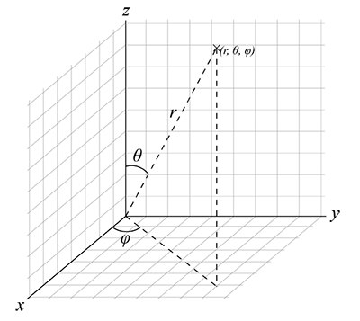
In a spherical coordinate system, the angles are the coordinates. So, if I were standing in a field in North Dakota, looking at something tall like an enormous wind turbine, I could define the position of the top of the nacelle relative to me by stating the general azimuth angle (, the rotation across the horizon from due South) and the general altitude angle (, the rotation up from the horizon). Effectively, this is my x () and y () coordinates on an orthographic projection of the sky dome on a flat surface.
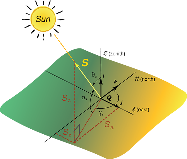
Many of you will be familiar with Cartesian coordinates in space (x, y, z). However, when dealing with spatial relations of spherical objects like the Earth and the Celestial Sphere, we find that working with basic spherical coordinate systems makes trigonometry available to us to solve for space and time equations. For spherical coordinates, we need information of radial distance, zenith angle, and azimuth. However, in solar positioning studies, a radius of one (unit radius) is all we need to establish a unit vector, and we are left with equations for only the zenith angle and azimuth (and the complement of the zenith angle, the altitude angle). Note how the zenith angle in Figure 2.15, above (the generic angle), is congruent with the solar zenith () of the Sun, and the generic azimuth angle () is congruent with the solar azimuth ().
The following equations describe the Cartesian coordinates (x, y, z) for unit vectors, followed by the equivalent functionals using the complementary altitude angle.
As seen in Figure 2.16, we need to pull back to our old trigonometry mnemonics! Recall "Soh Cah Toa" when looking at the figure:

- Sine(A): Opposite over Hypotenuse (a/h)
- Cosine(A): Adjacent over Hypotenuse (b/h)
- Tangent(A): Opposite over Adjacent (a/b)
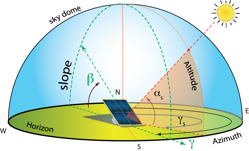
2.13 Sky Dome and Projections
Sun Charts: Projections of Solar Events and Shadowing from the Sky Dome
The emphasis of this lesson is the Sun Chart tool (or Sun Path). These flat diagrams are found in many solar design tools, but may look completely foreign to the new student in solar energy. How do we interpret the arcs and points plotted on a sun chart? Why do we have two different types of plots (one looks like a rectangle, and one looks like a circle)? Why do some plots go from 0-360°, while others go from -180° to +180°?
Video: Angles Sunchart 1 (4:45)
OK, we're going to do a little preliminary review of where we've been and why these angles are important to the measurement or the plotting of sun charts. So, we know that we have a set of several earth, sun angles. So, earth, sun angles. Excuse my wonderful writing. And we're going to break those down into the latitude phi, the longitude.
So, we've got latitude and longitude. And we're also going to need the declination, the declination which is going to be a function of the day number n, and the hour angle. And the hour angle, again, is omega. And that's going to be just converting time into an angular value, which we do for the location at hand.
So, along with those earth, sun angles, we have our sun observer angles. And the sun observer angles is going to be broken down into just three simple angles which is going to be the solar altitude, altitude angle alpha with the subscript s relating it to the behavior of the sun. Gamma s is going to be the azimuth angle of the sun. And the third angle is going to be theta z which is the zenith angle for the sun.
Now, I'm going to use the information from latitude, longitude, declination, and hour angle to ultimately calculate the sun observer angles over here. The important angles for our future shading plots and for our sun path diagrams are going to boil down to plotting altitude and azimuth.
So, we're going to use these earth, sun angles to calculate sun observer angles right here. And if we plot those angles over the course of the day, over the number of hours in a day, we're going to ultimately plot the altitude and azimuth angles according to their hour angle. And the complement, of course, of the altitude angle is the zenith angle. I forgot to mention that.
But we're going to be able to make these plots that are going to look like this. They're going to be a square plot where on the x-axis, we're going to have a plot of azimuths. And on the y-axis, we're going to have a plot of altitude angles. So, the altitude angle will go from zero to 90 degrees.
And depending on the system that we're using, negative values might be to the west and positive values-- or negative to the east and positive to the west. We could also plot here the complement. From zero down to 90 would be theta z, just so we know.
And again, if I plotted the solar altitude and solar azimuth angles, what I'm going to get is a plot of the arc over the hour angles. And this lower plot will be for winter, when the sun is low in the sky. Low in the sky means a low altitude angle. When the summer comes, the sun is high in the sky. And so, we have a higher angle in the summer.
And basically, this boundary from here to here is going to be the winter solstice and the summer solstice. These plots are basically plotting a series of altitude and azimuth angles for our sun charts. We will next be plotting a series of angles for shading that we will use.
So, that's our basic overview. Let's go on to the next stage.
What are Sun Charts?
If we want to visually convert our observations of the sky-dome onto a two-dimensional medium, we can either use an orthographic projection or a spherical projection on a polar chart. These projections are useful for calculating established times of solar availability or shadowing for a given point of solar collection.
The Sun Path describes the arc of the sun across the sky in relation to an earth-bound observer at a given latitude and time.
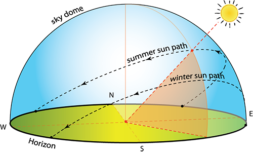
All light incident upon Earth's surface must pass through the atmosphere and be attenuated (lost from absorption or back scattering). In order to simplify the many points of origin of light, we divide the sky and the Earth's surface into components, or spatial blocks of an imaginary hemispherical projection on the sky. The Sky Dome refers to the sum of the components for the entire sky from horizon to zenith, and in all azimuthal directions. In our following sections, a collecting surface is assumed to be horizontal first, as a pyranometer measuring device is mounted horizontally and facing the sky to measure the Global Irradiance/Irradiation in the shortwave band for the sky dome. Most of our solar collectors will be tilted up from horizontal in some way (PV, solar hot water, windows, walls, even your eyes). Those surfaces oriented otherwise are termed a Plane of Array measurement (POA), requiring specific tilt and azimuth information in the description. For those solar collecting surfaces that are not horizontal, the reflectance of the ground is an additional source of light, through the albedo effect. The beam, sky diffuse, and ground diffuse light sources incident upon the tilted collector are estimated using models of light source components.
Projections
The sky dome can be projected onto flat surfaces for analysis of shading and sky component behavior.
Video: Angles Sunchart 2 (6:01)
So, if we go back and we think about the Sky Dome-- and I'm going to do this little diagram of-- this is the Sky Dome that we've talked about in the textbook and in the class. And this is going to be the ground. And so we have this Sky Dome.
And you can kind of see that this dome that we have could be-- is a hemisphere, first of all. And we could project that dome onto multiple different surfaces.
So, the first projection that we will do is going to be orthographic. And essentially, an orthographic projection is going to be what happens if I were to try to take a flat piece of paper. maybe like a cylinder of paper, and I were to try to wrap that cylinder right around this Sky Dome.
So, I'm going to have-- everybody see the cylinder that's wrapping around? So, I'm going to want to project points onto that flat surface. And ultimately, that flat surface is going to be printed out.
And we're going to have our basis for our sun charts in terms of the azimuth angle. So, the rotation along here, along the plane or rotation along the horizontal is the azimuth angle. And the angle from the ground up, the vertical rotation, is going to be the altitude angle.
Of course, the complement of that, if we were talking about the sun, would be the zenith angle. Which is why we could represent this is 0 to 90 and 90 down to 0 with the zenith angle.
We have two conventions for plotting the azimuth angle. The one is to make east negative. So, we can go negative 180 degrees. And west positive 180 degrees. Where this 0 is pointed at the equator.
The alternate is to begin in the north with 0 degrees and to work your way clockwise to-- all the way around to 360 degrees, in which case south, not the equator, is going to be positive 180 degrees.
Now, this is the convention that a lot of the solar world has used for some time. However, this is the standard convention that has been established through meteorology. And so, we tend to use both flexibly. But just know that, in general, the 360 degree is an accepted standard.
So, if we then go to the next page and we think about that same Sky Dome. And got our ground. And instead of trying to project it off to the side, we are effectively lying on the ground. And we're going to project upwards.
And this way, the azimuth angles are rotating around in a circle just like the azimuth angles will be doing here on the ground.
The altitude angles, however, are going to be represented as arcs across where the higher in the sky you are, the closer to the center of the circle.
And how do we see that? Well, we look at it like this. And we're going to start to see a center point. And I'm going to put south here. We know that south is in the northern hemisphere where the sun is at its highest point.
So, we're going to see arcs in the sky that look like this going from-- in our case-- east to west. This is going to be summertime. This is going to be wintertime. When the sun is low in the sky versus high in the sky.
Here is going to be an alpha 90 degrees. And the ring around the bottom is going to be an alpha of zero degrees. It's a little different plot. The lines are going to be flipped from what you were used to in an orthographic projection, if you can do both of these at the Oregon site for sun plots.
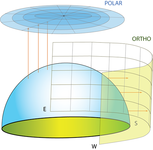
- Orthographic Projection: takes the sky dome and projects altitude and azimuth values outward onto a surrounding vertical cylinder. The cylinder is then opened flat. Figure 2.19, below, shows the sun rising in the East (to the left) and setting in the West (to the right). Proper observation shows that the largest arc in the chart at the top, June 21, is the Northern Solstice, while the smallest, December 21, is the Southern Solstice.
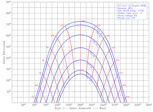 Figure 2.19: Orthographic Projection.
 - Polar Projection: takes the sky dome and projects altitude and azimuth values down onto a circular plane. However, in the polar projection, the arc for December 21 is at the top while the arc for June 21 is at the bottom. This happens because we are effectively lying on the ground with our heads facing south, and holding that large piece of paper straight up to the sky.
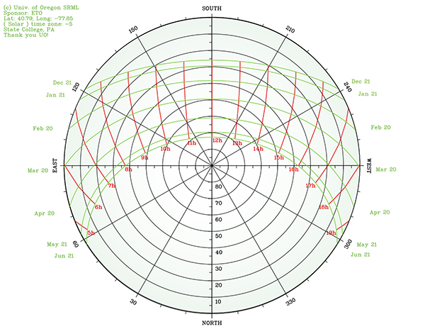 Figure 2.20: Polar Projection
How do We Make and Read Sun Charts?
Go to the University of Oregon Solar Radiation Monitoring Laboratory [27] website. The scientists at the site have provided an excellent tool for plotting sun paths onto orthographic projections or polar/spherical projections. The default page is for creating an orthographic projection of your site of interest. The alternate page for polar projections [28] will use the same data you can input, but will output the alternate form. Note that both use the meteorological standard for azimuth angles, where North is set at 0°, increasing clockwise to 360°.
- Specify the location by and . (Latitude is important for our calculations of sun-observer angles).
- Specify the time zone (software does the correction from UTC to local time zone).
- Choose data to be plotted (Choose to plot hours in local solar time: default). These plots are symmetrical for half of the year when you plot them in arcs of solar time. Hence, when you plot in solar time, "Plot dates 30 or 31 days apart, between solstices, December through June" will look the same as "Plot dates 30 or 31 days apart, between solstices, June through December." Side note: if you do plot in "local standard time," you will observe half of an analemma each hour, where only the Equation of Time ($E_t$) has not been corrected for in the time correction.
- Set chart format parameters: These are your choice to personalize the output file. Be creative, and try to present clear data visualization.
- Choose file format for chart. (I prefer the PDF for working.)
- Enter the code to make sure you are not a web bot roaming about.
- Download the image, print it out, and use it for shading analysis!
What about Shadows?
When designing a solar energy conversion system for any application, we must pay special attention to the occurrence of shadows throughout the year. We discuss a method to assess the shading using 2-D projections.
The next page gives you an opportunity to print and analyze your own sun chart.
2.14 Try This! Print a Sun Chart
Try This! - Print a Sunchart.
Go to the University of Oregon Solar Radiation Monitoring Laboratory [29] [27]web page and generate a PDF SunCharts for two locations: (1) State College, PA, and (2) your own location.
1. Download the PDF chart for the orthographic (Cartesian) projection
2. Download the PDF chart for the polar projection
3. Reflect on the charts:
- Can you find key solar days on the chart (equinoxes, solstices)?
- Can you identify sunrise and sunset solar times for different months?
- How does the position of sunrise and sunset vary throughout the year?
- How are these charts different between your location and State College, PA?
Now, based on your understanding of the SunCharts, work through the self-check questions below. While you work through these steps, try to think about all the calculations that went into each plotted point on the curves. You should reflect on the fact that the SunChart tool is simply plotting points and lines based on solar calculations of time and longitude. The same calculations that you are mastering now in class. Pretty exciting!
Self-Check Questions - based on the SunChart for State College, PA
Answer the same questions for your own locale. Are the answers different or the same compared to State College, PA?
2.15 Applying Shading to a Solar Chart
Reading Assignment
- SECS, Chapter 7: Applying the Angles to Shadows and Tracking
Here, we are going to work through a problem of plotting critical points of shading onto an existing sun path diagram. Keep in mind that we will use the plots that you developed from the University of Oregon Solar Radiation Monitoring Laboratory [29] on the previous page of this lesson.
Here, I am using a program called Skitch [30] to draw over the top of my PDF files. There is a 30-day free trial of the editing software if you would like to use it to digitally mark up your documents. Otherwise, I recommend that you print out your work, draw on the print directly with a pen, and then take a snapshot of the edited image with your phone or scanner to upload.
Quick review of the Charts:
First, we will go over the key features of the orthographic plots with the arcs of six days plotted out for the first half of the year.
Video: Sunchart Ortho Intro (4:42)
All right, so, here we have a sun path diagram of State College, Pennsylvania. We've developed this in the University of Oregon's website for our local latitude and local longitude, time zone UTC minus 5 hours. That's Daylight Standard Time, not Daylight Savings Time. And I've done a little bit of modification to this to give it the green background. So, this is not something that normally you would see inside of your normal program.
But, I want to point out a few things. One is that we see that, as discussed before, the sun rises in the east. And the sun sets in the west, right?
So, we're going to have a progression of the sun across the day from left to right. In this particular case, we start out with east on the left, west on the right. South is denoted by 180 degrees, right?
And so, the thing that I wanted to point out here is that here we have December at the bottom and June 21 at the top. So, this December 21 is the winter solstice. June 21 is the summer solstice. And, in between, we have right about March 21 through the 23 is going to be one of the equinoxes. The other equinox, of course, is going to happen in September.
Only half of the year is shown. The arcs that you're seeing here are all the hours of the day interpreted as solar time. So, this is going to be 10 o'clock solar time. We're using a 24-hour system here. So, this is going to be 2 o'clock solar time, right?
And when I look at this, I see that I have two key points-- 90 degrees and 270 degrees. 90 degrees, of course, is going to be due east. And 270 degrees is due west, in this particular meteorological standard for the azimuth directions.
We see that on the left side, we have the altitude angle. That would be alpha. And we're counting down for the zenith angle, the complement to the altitude angle.
Let's go back to this east and west. So, when does east happen? East happens at due east, is 90 degrees. Due west is 270 degrees.
What's really important here is when does that happen? You see that there's an arc right along here for March 21. And that's really close to the equinox. So, during the equinox, we have the sun-- that's the only time of the year-- so, two times during the year when the sun rises due east and sets due west.
And if we count the hours, we have-- one, two, three, four, five, six-- exactly six hours in the morning-- one, two, three, four, five, six-- exactly six hours in the afternoon, so, a 12-hour day, our only 12-hour day that's going to happen. Otherwise, all of the rest of this time if we're looking at-- let's grab a color here. If we're looking at all of this time of the year from December to February and after March, so, before March is down here. After March is up here. So we're going to have short days, shorter than 12. And we're going to have longer than 12 hours up in the summertime.
Gives you a brief breakdown of what's happening on orthographic projection. This is for State College, of course. As we go further north, we're going to see that our sun charts are going to get lower to the ground.
If we were to choose a latitude location that is closer to the equator, we're going to have plots that start to look like this, actually. They're going to look really kind of funny because they're going to spread out up into the 90 degree space because once you're within the tropics, you're going to find that the sun can be to the north or to the south. It's not always in the south as it is when you're beyond the tropics. Anyway, I hope that's a helpful explanation and--
Second, we can compare the key features of the orthographic plots to the polar plots, again with the arcs of six days plotted out for the first half of the year. You should notice the similarities (East is on the left, solar time is represented, the same location is plotted), as well as the distinct differences (the June and December arcs are "flipped").
Video: SunChart Polar Intro (5:49)
All right, and now we got the same location. Again, the location is going to be State College Pennsylvania. Solar time is going to be minus 5 hours, relative to UTC. And latitude longitude is the same.
Again, this is a polar plot of the same data that you just saw in the previous video. And the north of this plot is right down at the bottom. The south is up at the top. And I do this in this particular case, just to keep the arcs in the same general direction. But you're going to notice some differences here.
One is that the June arc is at the bottom. Whereas the December arc is at the top. So, this polar projection is what you would get if you were effectively lying on the ground and looking at the sky with a fisheye lens. And then trying to project that flat.
So, we see here that we've got the arcs of the day the morning begins over here. The evening ends over here, right in June time. And the progression of the day is going to be across the arc, again, from left to right, the same thing as we had before. Left to right in the winter months as well.
But here, you're really seeing the differences in the length of the day. It's probably a lot more apparent here that the length of the December 21st day is much shorter of an arc then the summer solstice on June 21st. Again, our arrows just pointing out, these green arcs are days. And the red lines are the hours of the day in solar time.
So that this top location here at 90 degrees, is going to be the top of the sky, the zenith. So, the zenith angle is basically any angle down from here to one of these circles. Whereas the altitude angle is going to be the angle up from the ground, which is going to be in our case the edge of the ring up.
So, we're going to see in a zenith angle going down or going outward, two rings. An altitude angle coming up or inward, basically coming along the edge of that skydome. And any one of these points of these green arcs are going to be a combination of an altitude angle and a azimuth angle.
And here, the azimuth angles are going to rotate from North which is zero degrees. North right here, is zero degrees. Rotating along to plus 30, plus 60, to finally when we're due east we are at 90 degrees. When we are due west, we're at 270 degrees. South in this case, is going to be 180 degrees. So, the azimuth rotates around clockwise and 180 degrees is in the meteorological standard going to the south.
Again, I want you to pay attention to the one day of the year when the sun rises due east and sets due west. And that's going to be around this, March 21st through the 23rd. It's kind of a flexible date depending on the year.
But it basically is defined as the day when within which the equinox occurs. And so, it's going to be one of the few days, or the only official day that you're going to have twelve hours of sunlight. So, we can count again one, two, three, four, five, six hours in the morning; that's going to mirror to the six hours in the evening making it a 12 hour day.
And again, that means that we're going to have everything in the summer is going to be longer, whereas everything in the winter months is going to be shorter. And that's the flip that I'm talking about in the notes, that the arcs flip back and forth. So, long days are on the bottom, short days are on the top, or short days are towards the south.
This should make sense when we think about the fact that the sun is low in the sky, low in the sky is going to be closer to the outermost rings. The sun is low in the sky in the winter. The sun is high in the sky, especially around the noon hour, during the summer.
And you're seeing that right here, is that the closer I am to this center ring, the closer I am to right here. Which is 90 degrees, the higher in the sky that I am. And so, in the winter time, I'm close to the perimeter, which is close to zero degrees altitude angle. This up at the top is close to 90 degrees altitude angle.
How to integrate shading as an overlay
Now, we need to add an additional layer of information to the plot. I'm going to talk through the addition of critical points on the sun chart, followed by connecting those points and shading the areas correctly. In each of the following examples, we will use orthographic projections, but there is no reason why you couldn't use polar plots instead.
Note
We are not plotting what the shadow "looks like." Instead, we are plotting the times over the course of a year (or half-year) for which a shadow exists on our receiving points of interest. We know that the actual shadows on a building are rectangular in shape (or have straight edges). However, the plot of the times in which shading occurs will not necessarily be rectangular.The first example will come from the textbook. We will be plotting shading relative to a single receiving point: X, with three critical points of shading (A, B, and C).
Video: Shading Wing Demo (5:52)
So now, we want to plot some critical points. And I'm going to go back to what you already encountered in the textbook in Chapter 7, applying the angles to shadows and tracking. So, let's focus on shadows. The first example that we've got here is the example of a wing wall, a wing wall being an extension out from the side of a building that might be blocking the sun. In the case that we've got in the textbook, we've got a wall that is to the west of the site.
And so, in our case, that means that on this plot, it's going to be a shadow that's going to be occurring on the west side in the afternoon sun. And we'd like to plot when is that shading going to happen on our central point, our point of interest, x. In this case, x was in the center of the building. So, we can imagine that this is a window that we wanted to understand-- or a central point in the window-- and we wanted to understand when is it being shaded versus not shaded.
And so, we did some basic trigonometry in the textbook to give us critical points between the central point, x, and three other shadowing critical points, A, B, and C. And those points are listed in the textbook. And so, what I'm going to do right now is just start plotting those out. And so, we had our points in that case listed as 0 being the south.
And so, when I had plus 54 degrees, what I was having is in addition of 54 degrees onto the original 180 degrees. And so, we're going to end up with some points at the bottom. And they're going to go up to our critical point of A, which was 0 degrees-- altitude angle-- 0 degrees altitude angle and 54 degrees to the west, to the afternoon azimuth angle.
And then point B was going to be a separate altitude angle upwards of 35 degrees. So, let's grow to approximately 35 degrees. We'll plot a second point right there. And our third point-- so, this was point XA. This point was point XB.
And now we're going to need a third point that's going to be point X relative to the critical point, C. And that was going to be 45 degrees up, so, we count up 45 degrees. And we're going to go up 45 degrees. And we need to go into the west in the azimuth 114 degrees. So, first, we had 100 degrees. And then, we're going to get about 114 degrees across to finally get our critical point, C.
So, if I want to connect these guys together, the first thing I know in an orthographic projection-- and I'm just telling you this-- is that it's a vertical drop down. So, lines connected together vertically will basically just have a vertical line down. The connection for the points here is going to be more like an arc. And so, we make sure that we have a nice arc tying these points together.
And I'm just going to extend continuously out towards the north. And then, I'm going to shade that data in under here. So, all of this region is going to be under shadows or our wing wall. So, we understand that in December, we get shading happening at about 4 o'clock in the afternoon. So, 4 o'clock solar time shading happens for the rest of the day.
On March 21, shading is going to happen at about 2:50. And by the time we get to the other extreme, the summer solstice of June 21, that time is going to be about 3:45. So, from 3:45 on to the end of the day, we're going to have shadowing occurring for this particular point, X in the problem.
And now, if I were to take that same plot and show you what we did inside the textbook, it's going to look just like this. So, it's something very much like what the textbook is just by plotting the points out and connecting those points together.
In the next example, we will look at setting up the problem to assess a PV array shading problem. Our intent is to plot shading relative to multiple receiving points: A, B, and C, with three critical points of shading (1, 2, and 3). The result is nine values for altitude coordinates ( , no subscript) and nine values for azimuth coordinates ( , no subscript).
Video: Shading Array Demo 1 (6:08)
So, here we have the scenario of an array of photovoltaic that are set up one row behind the next. They're each going to have a certain tilt. That tilt is represented by beta and each one is going to have a common collector azimuth of gamma, represented down here. And that gamma again, is that plane or rotation. In this case, the array that you're seeing is rotated 9 degrees towards the east. So, minus 9 degrees of rotation or 9 minus 180 degrees to give us our azimuth.
The distance between the panels, right now it's just specified as D. And the panels themselves are going to have a shadow. And that shadow is going to change over the course of the year, as the sun is high in the sky, and low in the sky.
And what we'd really like is for these panels to be spaced appropriately. Such that, they do not block each other. Because this is one of our goals, one of our mechanisms for the goal of solar design. You want to maximize the solar utility for the client or stakeholders in a given locale. And in this locale, want to know how far apart we can space these to collect the energy to basically avoid, or remove shading from the spacing of these panels.
So, what you're seeing is a system that we're going to define in terms of critical points. We're going to take those critical points and we're going to plot them on a diagram. So, the first thing is, how do we list these critical points. Well, now, we don't have a central point X.
Now, we actually have three points for each one of the panels across the top and across the bottom. This guy is going to be behind here, you won't see it. But you're going to have three points along the bottom, three points along the top. The points along the top are ultimately going to shade these critical points along the bottom.
So, I'm going to name these critical points A, B, and C. And the points that we will be referring to in terms of what kind of shading are we expecting, we're going to label 1, 2, and 3.
So, now, going into this, you're looking at this from the side and you're seeing a system like this; there's going to be a certain tilt beta. The beta is going to be the same from both collectors and they're going to be separated by a certain distance D. That's either going to be the spacing from top to top or from bottom to bottom, that's the same spacing with D.
So, looking at this, we want to basically compare any point 1. And what we really like to see is, how does 1 compare to point C, point C is down here. One to point C, 1 to point B, and 1 to point A. That's one of our first questions.
And then, after we've done that, we're going to look at how this point 2 compares to critical point C, critical point B, and A. And then, we'll finally finish that with 3 C, 3 B, and 3 A. And what we should be able to see is that because of similar geometries, we're going to find some kind of similar responses, in terms of all of these geometric relationships.
And I can show you that, again this is in the textbook, but if I bring this up right here, you're going to see that I've got a table of points 1.A, 2.A, 3.A, just like what we were talking about. And 1.B, 2.B, 3.B, 1.C, 2.C, 3.C. They each have their own set of altitude angles, and you're going to notice that there are certain 21 degree common altitude angles. Just due to common geometries. Similarly, you're going to see common 41 degree angles and two 12 degree angles.
Looking at the azimuth angles, the 0 degree azimuth corresponds to 180 degrees in the meteorological standard, and so on down. So, we're seeing that 76 degrees is equivalent to 250 degrees. And minus 64 degrees is equivalent to 116 degrees.
So, we're going to take these points this 180, 244, 256 for the azimuth angles of the collector. And we're going to plot those in the next block and we'll plot the alpha angles. And what we're going to come up with is basically something that looks like the cross section of a loaf of bread. It's going to have two vertical sides and it's going to have an arc in the middle.
You will notice how the horizontal surfaces of the building that create shadows are transposed to the projection as an arc, not as a horizontal line, while the vertical surfaces remain vertical. This has to do with the manner in which spherical data is distorted in an orthographic projection. Hence, the plot of a building shading a point on a window will look a lot like a slice of bread, flat on the sides with a soft curve across the top. The same will be found for this example, where the receiving points A, B, and C are shaded at different times by critical points 1, 2, and 3.
Video: Shading Array Demo 2 (5:57)
Now, we transition to plotting those points for the two rays onto our sun path chart. And so, here we have our sun path. It's again, I'm just using it for State College. You could use it for your location, in which case, the times at which you're actually going to be shadowing each other are going to be different.
So, if I go to my table from the textbook and I look at 1a, 2a, 3a-- I'm going to do those in blue first-- I'm going to get alpha values at, first, 180 degrees azimuth. And I'm going to go up 41 degrees for 1a. Then I'm going to go to 244 degrees azimuth, or 64 degrees from the convention in the book, up 21 degrees.
All right, 244 and 21. And I'm going to go down to 256. So, 256 is 76 degrees, and down to 12. So, somewhere right around here is where I'm looking at.
That plots the three points for 1a, 2a, and 3a. If I go over to 1b, 2b, 3b, I'm going to need to go to 116 degrees and then up 21 degrees. That's going to be for 1b. I'm going to need to go 180 degrees and up to 41 degrees, the same point as 2a. And then, my final point is going to be 21 degrees up and 244 degrees over.
So, again, we've got common overlap there. We're going to see this a couple of times. So, now, let's go to our last set of points. And that was going to be the 1c, 2c, and 3c. We're going to do those in green. And that's going to be 12 degrees up at 104.
So, that's probably going to be the mirror image of this point right over here, point 3a. And we're going to also look at 116 degrees 21 degrees up. That's an equivalent point, also.
And finally, our third point is going to be 180 degrees and 41 degrees up, which again, as we saw, is a common point for all of these. And so, when I connect these together, I'm going to go to my farthest point on each edge and drop a vertical line down. This is vertical, should be vertical. And then, I'm going to draw this loaf of bread arc between all of them.
It might not be pretty. In fact, I might do that one again. Let me just connect these points. Oops. Like this, back down. And then, finally, connect it together.
So, everything under this curve is going to be in shadow. And so, what we are seeing is that the months for this particular array, the way that it was designed, you're going to see that-- if I just look at the analysis of this-- you're going to see that even up to March in the winter months, definitely throughout the entire month of December, you're going to have the photovoltaic array shaded, which is not a good sign. And, again, into the afternoon of March, we're going to have shading.
So, we're going to see some distinct shading possibilities for this array, suggesting that when we actually want to develop this array, we'd want to space the array further apart. And to what degree would we want to space it further apart, we'd effectively want to look into how do we get this array spacing to be far enough apart so that the loaf of bread top fits underneath this area where it's not blocking any of the months in the hours of the day. And we can do that with effective design.
So, right now, as it's designed, the front array is going to shade the rear array. And that's going to create a problem. And we can count the number of hours that shading is occurring in that period. And we could enter that data into our system adviser model into SAM and then run the simulation to find out what the losses would be relative to no shading in that system. And we're going to do that in the next page.
Next, we will be interpreting our results, and inputting the shadow data into SAM.
Note
In your homework assignment, you will be asked to do a similar procedure for the solar array, but with the use of the polar projection of the SunChart, which provides somewhat better accuracy for determining the shading factors. While the solar coordinates are positioned differently in the polar projection, the principle of plotting critical points is the same - you find the positions for the points and connect them to define the shade/no-shade boundary. See an additional video demo on this in Canvas.
2.16 Applying Shading Factors in SAM
System Advisor Model
I hope you were successful installing SAM software and getting it ready to use in the last lesson. Now you will be applying your interpretation of the shading diagram to determine shading factors and input them into SAM for system energy performance simulations where shading interferes with the solar resource.
We have come a long way in interpreting sun path diagrams and plotting shaded areas as overlays onto the sun path charts. How can we input those shade/no-shade conditions to the PV performance model in SAM? The video below provides a demo of how shading conditions can be applied in SAM simulations.
Note
This video is made using the 2020 version of SAM. In newer versions, some tab specifications may differ.
Video: SAM Shading Intro (6:26)
How do we apply shading factors in system advisory model? I'll show you just in a second. I'm using System Advisor Model SAM, version 2020, and I'm going to start a new project. Here button on top-left. And for the example of the solar array given in the lesson two assignment for EME 810, we will need to choose photovoltaic long left side menu of options for my system. But you will not need all of them for this assignment, you actually will need only a few. Location and resource where you set location for your project. Then system design where you can tweak some of the parameters of the system and obviously shading, because that's where we apply the shading factors. Okay, let's go one-by-one. Set things up for it. First.
In the assignment, it states that the system we're working with is located in Baltimore. So, we need to find that location. I have Baltimore in my weather file library if you don't see one in yours, So, you may just go down here and search by location and pull that file into a library first. So, once I click on it, I also see it appearing down here, weather data information in Baltimore, so it's good to go. The system design. We can set the parameters of the system close to what we have in the assignment. So, I can set the nominal capacity for the systems here. It's four kilowatts. So, I'll leave it at that. And also, if I scroll down, I can put the tilt 35 degrees and azimuth for the system close to the ones that are described in the textbook and described it in the assignment. So, the system is oriented nine degrees east of the two south, so that would give me 171. And that's all I need here.
Now to shading. On the shading options. The area you want to look at is this, shade loss tables. If you click on edit shading, it will give you a number of options and how you input your shading data. And the one you need is enabled month-by-hour beam irradiance shading losses. So, click here, and now it brings up this table that you can use to input your shading factors for each month of the year from January to December for each hour of the day. How to use this table. It's very easy. If you have no shade, you leave it at zero, which is default. You have full shade. You need to enter 100%. Like this. And it's, your area will be shaded. You can also apply to multiple cells, for example if, I'm sure that my area will be shaded 100 per cent, for months of January and February, I can apply that 100 shading factor for all those cells for both months. The same way, I can apply it to any other months of the year. Like October through December, for example. Once I have those factors setup, I click Okay, and I go to simulation.
The output of the model shows me the annual energy here from my system in kilowatt hours, shows the capacity factor, and monthly energy profile. You can also print this monthly data in the table. For that, you would need to go to data tables here on top. Choose monthly data. Scroll all the way down through all those many variables. You need system AC energy kilowatt hours per month. Click here. And wallah, you have January through December, your output in kilowatt hours.
If you add them all up, you should be getting that annual energy that was given in the summary here. For this assignment, you will need to model your system for both shaded and nonshaded scenarios. So obviously you can go back and modify this table. I can apply zero to all cells here, indicating no shade. This will be my baseline. Click. Okay. And I simulate again. You see the profile of the energy output changed significantly. So, your goal will be to compare those two scenarios and find out how much shading losses you would have.
So, the important take-aways are that we can use SunCharts or other geometric shading data to get us to a shade-based performance adjustment of PV performance simulations, and that shading matters in solar energy. How significant can it be? Quite significant, but you will get a more accurate answer after performing your homework assignment in this lesson! We use these SAM simulations in solar project design, and this will be the way to assess the shading losses for any specific scenario (and in your final course project, eventually).
When working with SAM shading table, we can input partial values for hours that are on the shade/no-shade borderline (e.g. 50% etc.). SAM conveniently grades the color scheme from white (full sun) to red (full shade) in the process. Also, note that the locale matters! Do not forget to set your location in the Location and Resource tab first: the default for SAM is often in the Southwest USA, and you will need a correct solar resource file before running your simulations.
2.17 Learning Activity
This activity allows you to apply the concepts of time and space coordinates you learned in this lesson to a specific example of a solar energy conversion system. In the process, you will work with both Sun Chart and SAM software to model the performance of a PV array. You will be required to demonstrate your learned skills for Sun Chart interpretation, shadow tracking, and including shading information into SAM simulations.
PV Array System
- A fixed-axis array of PV modules installed in the Baltimore MD area.
- The array consists of two rows of 8 modules stacked together (see more description and picture in Chapter 7 of the SECS Book), each module is 1.25 m in height and 1 m wide.
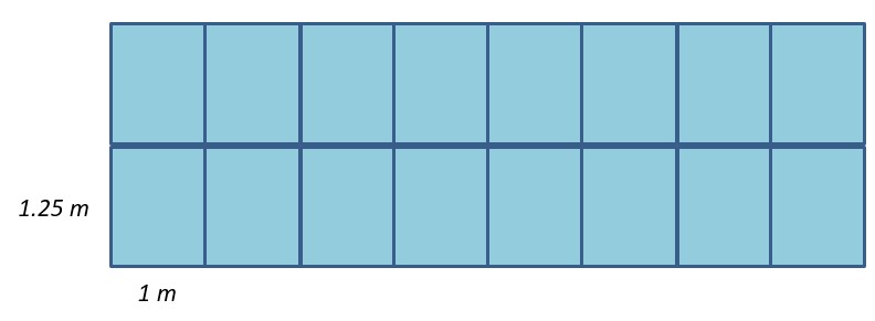
- Orientation: azimuth -9o (i.e. it is facing a few degrees East of South)
- Tilt: 35o (fixed)
- The array is assumed to be part of a larger solar installation, meaning that a similar array positioned in the front can cast shadow to our array of interest.
- Spacing between the arrays in the field is 3 m.
- Nominal array capacity 4 kW
- Assume PV cells and modules are connected in series, so partial shading along the base will affect the entire array (simplified case).
Task
Model the effect of shading on the PV array performance (kWh of energy generated) over a year. So, in the end, you will need to produce the energy output data from the array for the full-sun and shaded scenarios and observe the difference.
Directions
- SunChart. Create the Sun Chart for sun trajectory of the Baltimore, MD, location using the University of Oregon Solar Radiation Monitoring Laboratory solar tool. [29] You are to use the polar sun chart in this activity. Download your Sun Chart diagram as a PDF file. You have seen examples of this in the videos included in this Lesson. You will use this chart further to put your shading information on.
-
Apply shading. Study the “Array Packing” example in Chapter 7 of the J. Brownson’s SECS Book, understanding how shading coordinates can be obtained for a specific system geometry. Plot all the critical points by shading coordinates given in Table 7.3 on your Sun Chart. Connect the points and show the shaded zone on your diagram (see lesson videos and textbook for more guidance on how to do it). You can use a graphics software for this purpose or do it by hand if that is easier.
NOTE: the solar azimuth coordinates used by SunChart are different from those Brownson's book. The former considers 180o as true south, while the latter considers 0o as true south. So, you would need to convert the solar azimuths from the book by adding 180 in order to correctly plot the points on the SunChart. -
SAM Simulaton A (you have already downloaded SAM as instructed in Lesson 1):
- Start a new PV project in SAM – choose Detailed PV Model - Residential Owner option when initiating a project
- Under Location and Resource tab, input Baltimore, MD
- Under System Design tab, input specifications for the system (4 kW nameplate capacity, array tilt and azimuth)
- For the first round, do not include shading data
- Run the simulation by pressing the blue 'Simulate' button at the bottom left of the screen
- To get the monthly energy data in table, click on DataTables tab on top. Then choose output variables: you need Monthly Energy (KWh) and total Annual Energy (kWh) for a single year. You can also find the latter by just summing up your monthly values.
- Export your table to an Excel spreadsheet
- Sam Simulation B. Repeat the same simulation as described in Step 3 now including the shading data. This is how: Save your project as a new file. Under 'Shading Layout' tab, click 'Edit Shading' button. Then, in the editing window, choose the option ‘Enable month by hour beam irradiance shading losses’. You will be given a table to input shading factors for each hour in each month. For simplicity, we will consider the same (averaged) shading factor for all days in the same month. Looking at your Sun Chart, input 0 for no shading, 100 for full shade, and 50 for borderline or changing conditions. Once done, run the SAM simulation and export data table as described in Step 3. (See demo video in Canvas for this step)
-
Discussion. Provide a brief discussion comparing your shaded and non-shaded results and what you learned from this activity.
Submitting Your Work
Prepare a written report including the following results:
- Sun Chart for Baltimore, MD with critical points and shaded zone plotted on it.
- Table of SAM simulation results for full sun and shaded scenarios. This table should contain monthly energy generated as well as total annual energy delivered by the array. In your energy performance table, your numbers should be rounded to the nearest whole kWh (no decimals).
- Screenshot of shading factor table from SAM.
- A paragraph with a discussion of your results.
Upload your report file to the Lesson 2 Learning Activity DropBox in PDF or docx format.
Grading Criteria
- Sun Charts (10 pt). This part will be graded based on your ability to plot the calculated critical points and identify shaded versus non-shaded conditions for the system at the specific time and location.
- Energy Tables (10 pt). You will be given 1 pt per month based on the reasonable correctness of the numerical values. The purpose is not necessarily to get the exact "right" answer, but rather to have done the process and understand what you are doing. So discrepancies within +/- 30 kWh will not cause point deductions.
- Discussion (5pt).
- Screenshot of the Table with shading factors used for SAM simulation (5 pt).
Deadline
See the Canvas Calendar for specific due dates.
2.18 Summary and Final Tasks
So far, we have delved deep into the world of angles, time, and shading. Why have we done this? The solar resource is all about timing and placement of the SECS relative to the Sun, and the use of angles as coordinates in time and place are fundamental building blocks to the solar expert. We now have computational tools that make the work of calculating details trivial, but one must always know what the foundations are underneath those tools.
Who knows, maybe you will be the next open software developer to create a simple solar tool for resource assessment. You now have the keys to access many of those computational tools. More to the point, these fundamentals are not shrouded in mystery, and you don't necessarily need to pay for software to get access to them!
Looking ahead, I can tell you that students in residence at Penn State have already found a solar systems design plugin for Trimble SketchUp [31] called Skelion [32], which does shading analysis just like you performed, but on the fly inside of the SketchUp design software. Both are free to use, and I'd recommend you take a look at each in preparation for your end of semester design projects! This is an untapped resource for you to explore, now that you know "how" the shading calculations work.
Knowing these principles of angles and time also exposes us to the strengths and potential weaknesses of purely geometric relations in the solar resource. As we shall see in the next lesson, the role of the atmosphere and meteorology will tend to muck up our ideal angles of beams of light, and produce anisotropic (uneven) intensities of irradiance over the day, which will of course influence our solar resource estimations.
On to the next lesson--let's learn about the role of weather and the sky dome in estimating the solar resource!
The Goal of Solar Design and our Three New Mechanisms
The Goal of Solar Design is to:
- Maximize the solar utility
- for the client
- in a given locale.
Given the goal of solar design, we have learned of three mechanisms to leverage during the design process that will increase the solar utility for our client in their locale of interest:
- Reduce the cosine projection effect on an aperture/receiver (the extreme angles of incidence, or low glancing angles ),
- Reduce the angle of incidence on an aperture/receiver (refinement on minimizing ),
- Reduce losses from shadowing on an aperture/receiver.
In order to leverage these three tools, we have demonstrated that one needs to know where and when the Sun will be relative to our collector system.
Reminder - Complete all of the Lesson 2 tasks!
You have reached the end of Lesson 2! Double-check the to-do list on the Lesson 2 Learning Outcomes page to make sure you have completed all of the activities listed there before you begin Lesson 3.