Lessons
This is the course outline.
Lesson 1: Solar Energy Conversion and Utility Solar Power
Overview
Overview
Welcome to the first lesson of the EME 812. In this lesson, we will overview the main types and principles of solar energy conversion to usable outputs, such as electricity, heat, and fuel. There are quite a few technologies that help to do that. Some of those technologies are quite old and well-known, and some are still subject to current research. We will read a couple of recent review papers to learn about those technologies and their impact. Also, we will spend some time reviewing the concept of efficiency, which is a key metric of any process of energy conversion. Also, at the end of this lesson, I will ask you to refresh your knowledge of units and main terms used in the solar energy studies. Let's get started!
Learning Objectives
By the end of this lesson, you should be able to:
- Explain the basics of solar energy conversion;
- List examples and parameters of solar systems across the scale;
- Calculate efficiency of a solar system, based on system performance information.
Readings
Journal article: Crabtree, G.W. and Lewis, N.S., Solar Energy Conversion, Physics Today, 60(3), 37 (2007) [1].
Journal article: Hernandez, R.R. et al., Environmental Impacts of Utility Scale Solar Energy, Renewable and Sustainable Energy Reviews, 29, 766 (2014) [2].
L. Radovic, Efficiency of Energy Conversion [3]
J. R. Brownson, EME 810 Solar Resource Assessment and Economics. 2.2. Basic Solar Jargon for Energy and Power [4]
1.1 Solar Energy Conversion - Overview
1.1 Solar Energy Conversion - Overview
The energy that is naturally available from the Sun is quite enormous. The Sun delivers 1.2 x 10⁵ TW of radiative power onto the Earth, the amount that surpasses any other energy resource by capacity and availability. That would convert to 3.78 x 10¹² TJ of energy per year. For comparison, according to Crabtree and Lewis (2007), all recoverable Earth's oil reserves (~3 trillion barrels) account for 1.7 x 10¹⁰ TJ of energy. Thus, the sun supplies this amount of energy to the Earth in only ~1.6 days!
A few more stats:
According to reviews of University of Oxford [5], the current global energy utilization is close to 1.6 x 10⁵ TWh per year (i.e. 5.76 x 10⁸ TJ/year). If we again compare this amount to the global solar energy flux, the Sun is able to cover this demand in only 1 hour and 20 min! This is sort of mind blowing..
However, to be utilized, the solar radiation needs to be converted into other forms of energy, such as electricity or usable heat. The question is: can we effectively do that at the scale of our demands?
Evidently, the solar resource contains enough energy to cover those demands. However, the critical limitations in solar energy conversion will be the efficiency of existing technologies and availability of earth materials to scale up those conversion devices.
What's in solar spectrum?
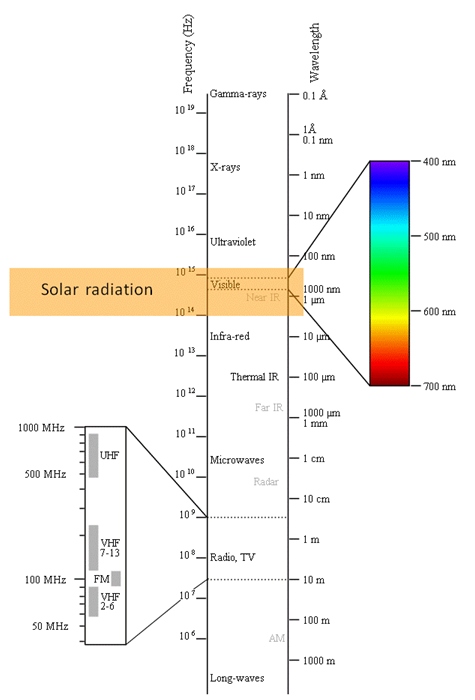
Before considering various types of conversion of solar energy, let us briefly review what solar radiation actually is. Here are a few main things we know from physics:
- Solar energy is electromagnetic radiation.
- Main components of solar radiation reaching the Earth (wave length, λ, range give in parenthesis):
- Infrared (52 – 55% λ > 700 nm)
- Visible (42 – 43% 400 < λ < 700 nm)
- Ultraviolet (3 – 5% 100 < λ < 400 nm) - see Figure 1.1
- Solar radiation near the earth surface is essentially in the range λ 290 – 2500 nm.
- Quantum (unit energy) of electromagnetic radiation - photon (E = hv) - is often a more convenient term in the mechanism of solar conversion.
Main types of sunlight conversion
This mix of various types of electromagnetic radiation allows the sunlight to be converted through a variety of physical mechanisms, which are:
- conversion to electricity (photovoltaic effect);
- conversion to usable heat (for example, via thermal collectors);
- conversion to matter / fuel (for example, production of biomass through photosynthesis).
Now we are going to take a closer look at various technologies that are able to convert solar radiation and learn what the main objectives and challenges are there.
Read the following article to overview the main types of solar energy conversion, and try to find the answers to the self-check questions below.
Reading Assignment
Journal article: Crabtree, G.W. and Lewis, N.S., Solar Energy Conversion, Physics Today, 60(3), 37 (2007) [1] - 6 pages
This article reviews the multiple possibilities to convert solar radiation into usable forms of energy. It discusses various ideas and recent advances in scientific research directed towards raising the conversion efficiency through better understanding the physicochemical phenomena.
Check Your Understanding - Essay Question 1
What is energy conversion efficiency? How would you define it in your own words?
Check Your Understanding - Essay Question 2
What is Shockley-Quesisser limit, and what is its value?
Check Your Understanding - Essay Question 3
What are possible approaches to reach higher efficiency of sunlight to electricity conversion in solar cells?
Check Your Understanding - Essay Question 4
What are possible approaches to reach higher efficiency of sunlight to heat conversion?
Check Your Understanding - Essay Question 5
What are possible approaches to reach higher efficiency of sunlight to fuel conversion?
As we perceive from this reading, numerous technologies and areas of research and innovation in solar energy conversion target the overarching objective to raise the device efficiency, thus making it more economically viable for implementation. This is especially true in the light of quite high capital costs for solar energy systems. This challenge is related to both initial materials and manufacturing.
We will talk more about efficiency on the next page of this lesson.
1.2 Efficiency of Conversion
1.2 Efficiency of Conversion
Efficiency is a very important metric in energy conversion. It is most commonly used for evaluating and comparing various methods and devices in terms of technical performance, which is, in turn, related to cost of the technology. The efficiency concept is frequently used in cost estimates and commercial decision making. So, we should spend some time refreshing our basic understanding of the efficiency as a universal metric of conversion systems.
Reading Assignment
Please refer to this Efficiency of Energy Conversion book chapter [3], and refresh your basic knowledge of the efficiency definition and use. This text uses a number of simple efficiency calculation examples related to traditional fuel systems. I encourage you to learn from those, and then we will see how the same approach may apply to solar energy systems and devices.
Based on this reading, can you answer the following questions?
Check Your Understanding - Question 1
If an electric motor consumes 150 W of electrical power to produce 120 W of mechanical power, what is the efficiency of this device?
Check Your Understanding - Question 2
How would you determine the energy conversion efficiency of a power plant that consists of three conversion sub-systems with efficiencies η1, η2, and η3, respectively?
Check Your Understanding - Question 3
A light bulb converts electric energy to light and heat. Can you estimate efficiency of a 40 W light bulb emitting 950 lumens of light energy (assume 1 lumen equivalent to 0.001496 W of power)?
We see that efficiency of conversion,η, is a key metric of system performance. When applied to solar energy conversion systems, efficiency of solar energy conversion would be defined as the ratio of the useful output power (delivered by the conversion device) to the incident power (of the solar radiation):
We can answer the following questions from the efficiency analysis:
- What fraction of available energy is lost in the conversion?
- How one device is compared to another?
- What is the performance limit?
PV efficiency measurements
When the efficiency is compared for different types of photovoltaic (PV) cells, we need to make sure that conditions under which the cells are operating are standardized, so that any difference in cell performance is due to the properties of materials and design and not due to the variability of external factors. The nominal efficiency of PV devices is measured at standard conditions [ASTM G173 guide]:
- Air temperature 25°C
- Solar irradiance of 1000 W/m2 (clear sky)
- Air mass (AM) of 1.5G
- Cell (panel) oriented perpendicular to the light beam
When the external conditions are kept constant, measured efficiency is solely a device characteristic. To determine efficiency experimentally, we need to measure both the solar irradiance and the power of the cell.
For your notes: [Solar Conversion Efficiency Cheat Sheet [7]].
Example of Efficiency Calculation
Generally, to estimate the efficiency of solar energy conversion, you would need:
- solar irradiance data, and
- performance data
Consider the example below, which shows estimation of the standard efficiency of a PV module.
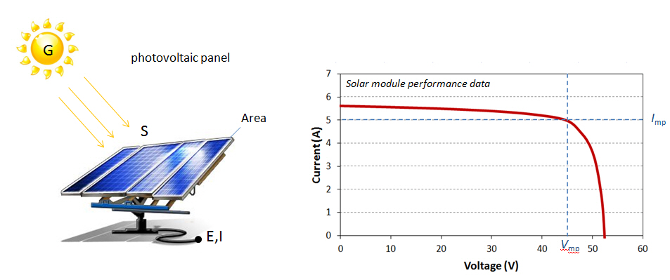
Standard solar input (irradiance) at the module surface: S = 1000 W/m2
Identifying power input to the PV cell:
Identifying power output from the PV cell:
(Note: from physics, power is equal voltage times current)
Then, for efficiency, we can write:
Conclusion: only 11.25% of energy flowing to this panel is converted to electricity.
The reason that energy conversion systems have less than 100% efficiency is that there are losses. The origin of those losses can be a complex issue, which could be better understood based on the physics and design of a particular conversion device – PV cell, concentrator, or thermal collector. We will get back to those considerations when talking about specific conversion technologies in detail in respective lessons of this course.
Quality and quantity of solar conversion
There is an important distinction between the total power (measured in Watts) and power density or flux (measured in W/m2). When we talk about the performance of a particular solar energy conversion device (for example, a solar cell), power density characterizes the "quality" of the energy conversion - how much power is generated by each square foot or square meter of the PV cell area. That may depend on properties of the cell material, design, and physical principles behind the conversion process. In contrast, the total power reflects the overall output - the "quantity" of usable energy generated by the whole device per unit of time. In applications of solar energy (say, if we want to power a building), we often look at the total wattage of the system and ways to maximize that total "quantity" of energy supply.
For example, imagine a solar module. At a particular moment of operation, the output power of the device can be expressed as
- η = efficiency (%)
- S = sunlight power density (irradiance) at the cell surface (W/m2)
- A = total cell area (m2)
Logically, to increase the total output from that module, we need to either increase the efficiency or increase the total input power.
The avenue of raising cell efficiency leads us to the physics of the conversion process, materials properties, and cell design. The main research and development question here is how to make a better working cell.
The avenue of increasing the total input power leads us to three issues: (i) concentration of light, (ii) sun tracking, and (iii) system scale-up. Concentrating the ambient incident light would indeed increase the amount of energy supplied to the module per unit of time via increasing the S parameter in the above equation. Tracking - i.e., the orientation of the solar panel perpendicular to the sunlight beam - is another way to maximize the amount of absorbable radiation and also contributes to increasing the S parameter. Finally, increasing the size of the module by adding more cells to the system, increasing cell area, or multiplying modules (scale-up) would increase the total active area of conversion (A).
The technology scale-up is the way to match the solar power to commercial applications and consumer's needs. The utility-scale solar power, which is the primary focus of this course, is discussed in the next section.
1.3 Utility Scale Power
1.3 Utility Scale Power
There are two main solar technologies that are being considered for large scale power generation: (1) Photovoltacs (PV) and (2) Concentrating Solar Power (CSP). Another type - concentrating photovoltaic (CPV) is currently not a major player, but there are a few large facilities that use CPV technology. PV and CSP are principally different in the type of energy conversion and type of solar resource they rely on. We are going to review the basics of those technologies and their current state in the energy market in this lesson before considering more technical details further on.
Photovoltaics (PV)
Reading Assignment
So, what do we mean by the Utility-Scale Solar Power?
Please read the introduction on the website of the Solar Energy Industries Association (SEIA) [8] and watch the video below to get the basic idea about utility-scale photovoltaic systems.
Video: Energy 101: Solar PV (2:00)
PRESENTER: All right, we all know that the sun's energy creates heat and light. But it can also be converted to make electricity, and lots of it. One technology is called solar photovoltaics, or PV for short. You've probably seen PV panels around for years. But recent advancements have greatly improved their efficiency and electrical output. Enough energy from the sun hits the Earth every hour to power the planet for an entire year.
Here's how it works. You see, sunlight is made up of tiny packets of energy called photons. These photons radiate out from the sun. And about 93 million miles later, they collide with a semiconductor on a solar panel here on Earth. It all happens at the speed of light. Take a closer look, and you can see the panel is made up of several individual cells, each with a positive and a negative layer-- which create an electric field. It works something like a battery.
So the photons strike the cell, and their energy frees some electrons in the semiconductor material. The electrons create an electric current, which is harnessed by wires connected to the positive and negative sides of the cell. The electricity created is multiplied by the number of cells in each panel and the number of panels in each solar array. Combined, a solar array can make a lot of electricity for your home or business. This rooftop solar array powers this home. And the array on top of this warehouse creates enough electricity for about 1,000 homes.
OK, there are some obvious advantages to Solar PV technology. It produces clean energy. It has no emissions, no moving parts. It doesn't make any noise, and it doesn't need water or fossil fuels to produce power. And it can be located right where the power is needed, in the middle of nowhere, or it can be tied into the power grid. Solar PV is growing fast. And it can play a big role in America's clean energy economy-- anywhere the sun shines.
Understanding the limitations in efficiency of solar energy conversion and taking into account the demands of centralized power generation, the technology scale-up is one of the important issues being developed by the government agencies in order to build sustainable energy future.
Obviously, there is a strong push for large-scale systems from the government and industry. But, along with the promise, the scale-up process brings new challenges to the energy conversion system design. Some of those challenges are:
- lower than desired efficiency (theoretical limits suggest it can be much higher);
- high up-front cost of materials and equipment;
- energy storage (electricity or heat);
- power distribution and transmission.
All these issues deserve more attention and will be covered in more detail in further lessons of this course. In this lesson, we are not yet digging into any technical details of the considered technologies but, rather, taking a plunge into the context.
The following materials will give you an idea of the current state of utility scale solar market in the US.
Reading Assignment
Industry Report: U.S. SOLAR MARKET INSIGHT [10], 2022 year in review, Executive summary, SEIA, Wood Mackenzie Power and Renewables, Published March 9, 2023.
The SEIA 2022 Market Report provides a general outlook of the role of PV solar technology at the scale of national energy development. In the year of 2022, solar accounts for 50% of all energy added to the national grid. However, unlike previous years, 2022 was dominated by the growth of residential solar (40%), while the utility sector had a slower progression due to some global market uncertainties and supply chain disruptions. Nevertheless, 11.8 GW(DC) of new capacity was installed for the year, further increasing the contribution of solar energy conversion into the US energy industry.
In more detail, photovoltaic technologies will be studied in Lessons 4-6.
Cencentrating Solar Power (CSP)
The other prominent technology developed on the utility scale in the US and worldwide is Concentrating Solar Power (CSP). While CSP is currently outpaced by PV on the global and domestic market, this technology may be advantageous in the areas with high annual insolation.
Watch this 2-min video to overview the utility-scale Concentrating Solar Power (CSP) systems:
Video: Energy 101: Concentrating Solar Power (2:00)
Ok Take the natural heat from the sun, reflect it against a mirror, focus all of that heat on one area, send it through a power system, and you've got a renewable way of making electricity.
It's called concentrating solar power, or CSP. Now, there are many types of CSP technologies. Towers, dishes, linear mirrors, and troughs. Have a look at this parabolic trough system. Parabolic troughs are large mirrors shaped like a giant "U." These troughs are connected together in long lines and will track the sun throughout the day. When the sun's heat is reflected off the mirror, the curved shape sends most of that reflected heat onto a receiver. The receiver tube is filled with a fluid. It could be oil, molten salt, something that holds the heat well. Basically, this super-hot liquid heats water in this thing called a heat exchanger, and the water turns to steam. Now, the steam is sent off to a turbine, and from there, it's business as usual inside a power plant. A steam turbine spins a generator and the generator makes electricity. Once the fluid transfers its heat, it's recycled and used over and over. And the steam is also cooled, condensed, and recycled again and again.
One big advantage of these trough systems is that the heated fluid can be stored and used later to keep making electricity when the sun isn't shining. Sunny skies and hot temperatures make the southwest, U.S. an ideal place for these kinds of power plants. Many concentrated solar power plants could be built within the next several years. And a single plant can generate 250 megawatts or more, which is enough to power about 90,000 homes. That's a lot of electricity to meet America's power needs.
Reading Assignment
Web article: 2018: The Year Sees Explosive Expansion of Concentrated Solar Power Capacity Globally [12], HELI SCSP, Accessed: April 2019.
While PV system significantly outpaced CSP in growth over the past decade, there is still a significant economic potential for converting solar thermal energy into power in a number of locations around the globe.
I hope these materials give you a clear idea what kind of systems will be the subject for learning in this course. The following self-check questions allow you to iterate the basics once more before we move ahead.
Check Your Understanding - Question 1
List the key technologies that have been involved in utility scale solar power generation:
Check Your Understanding - Question 2
How is the utility scale power different from the distributed generation power?
Check Your Understanding - Question 3
What were the top-3 ranked states for installing PV solar energy systems?
1.4 Environmental Impact of Utility Scale Solar Power
1.4 Environmental Impact of Utility Scale Solar Power
Utility-scale solar power installations are on the rise worldwide - the tendency fostered by advances in technology, new energy policies, and markets. Because of this growth, there has been an increased interest among stakeholders to understand the broader impacts of such systems on society and environment. In spite of the often idealistic public perception of solar technology as "green" panacea, an objective examination of the solar technology lifecycle reveals both positive and negative impacts. Careful impact assessment of large solar projects is important in order to steer the energy infrastructure development towards the optimal solutions that would take into account economic, environmental, and social values. Understanding the sensitivities and existing ecosystem services at the locale at the utility project planning stage is becoming a key step in responsible solar development.
Please read the following review article, which nicely covers the multiple effects of utility solar power.
Reading Assignment
Journal review article: Hernandez, R.R. et al., Environmental Impacts of Utility-Scale Solar Energy [2], Renewable and Sustainable Energy Reviews, 29, 766 (2014). - 11 pages
This article will be the background of the Lesson 1 forum discussion, and you will get a few questions on this material in the reading quiz (see the Summary and Activities page of this lesson for more details).
1.5 Refresher on Units and Terminology
1.5 Refresher on Units and Terminology
At the conclusion of this lesson, I want to refer you to some resources on basic energy units, conversions, and terminology that specifically applies to solar energy systems. If you have just completed the EME 810 course, you will find many of these things familiar. For example, can you clearly answer these questions:
- What is the difference between power and energy? And what are their units?
- What is the difference between power and power density?
- What is irradiance? What is irradiation? Is there difference?
- What are the symbols for irradiation on hourly and daily steps?
To get a better sense of solar language we are using here, feel free to check this unit from the EME 810 Course (Solar Resource Assessment and Economics) that explains the basic jargon and units used to measure solar energy and power.
Basic Solar Jargon for Energy and Power [4]
Also, it would be useful to look through the original technical paper by Beckman et al. (1978), too, and use it in the future if any notation questions arise. The main purpose of this material is for everyone to be on the same page when analyzing the solar energy conversion technologies further in this course.
Supplemental Materials:
These presentations provide additional explanations and illustrations to the concepts of energy conversion and efficiency. These resources are optional, but can be helpful if you need to revisit the basics.
 [13]
[13]
 [14]
[14]
Summary and Activities
Summary and Activities
Readings and activities in this lesson give you a general perspective of this course and set the context without yet addressing the specific science of the solar energy conversion technologies. Here, we try to figure out what aspects and what impacts would be important when the conversion technologies are scaled up to the utility level. Hopefully the materials of this lesson also provided you with a good refresher of such basic concepts and terms as energy conversion, efficiency, power, power density.
| Type | Description / Instructions | |
|---|---|---|
| Reading | Complete all necessary reading assigned in this lesson. | |
| Discussion | Discussion Forum "Environmental Impact of Solar Power"
|
|
| Reading Quiz | Complete the Lesson 1 Quiz. |
References for Lesson 1
Brownson, J.R., EME 810 Solar Resource Assessment and Economics. 2.2. Basic Solar Jargon for Energy and Power [4]
Crabtree, G.W. and Lewis, N.S., Solar Energy Conversion, Physics Today, 60(3), 37 (2007).
Duffie, J.A. and Beckman, W.A., Solar Engineering of Thermal Processes, John Wiley & Sons 2013.
Radovic, L. Efficiency of Energy Conversion [3]
Lesson 2: Concentration Fundamentals
Overview
Overview
In Lesson 1, we learned that the main function and purpose of the solar energy systems is to convert sun radiation - i.e., light or heat - into electricity. However, the efficiency of such conversion is not very high. One way to make many known solar technologies feasible with respect to their efficiency, total output, environmental impact, and cost is to concentrate the incoming radiation. Concentration of light will be the main topic of Lesson 2.
Sunlight is a practically inexhaustible natural resource which is also universally available. However, one of the disadvantages or difficulties related to its utilization is a relative low density of the solar flux. To generate sufficient power to meet demands of large populated zones, a vast area should be covered by solar collectors, and a significant amount of materials and resources should be spent on production and service of those collectors. This expense raises a question about economic viability of solar and initiates the search for ways to increase the sunlight conversion efficiency one way or the other. Generally, there are two ways to solve the problem - to improve the conversion device (intrinsic factor) or to increase the input flux (extrinsic factor). While the first avenue is subject to energy engineering research and innovation (e.g., developing new types of photovoltaic materials and devices), the second option - concentration of the incident solar flux - is already widely implemented. This lesson presents basic concepts for sunlight concentration and discusses typical optical geometries common in utility scale solar plants. This material provides background for further discussion of such technologies as concentrating solar power (CSP) or concentrating photovoltaics (CPV) later in this course.
Learning Objectives
By the end of this lesson, you should be able to:
- understand the physical principles of light concentration;
- list the main types of concentration systems used for utility scale solar facilities;
- calculate parameters of the typical light concentrating systems (CPC, parabolic concentrators).
Readings
Duffie, J.A. and Beckman, W.A., Solar Engineering of Thermal Processes, 4th Ed., John Wiley and Sons, 2013. Parts of Chapters 2 and 7. Please refer to particular sections of the lesson for more specific assignment.
2.1 Available Solar Radiation and How It Is Measured
2.1 Available Solar Radiation and How It Is Measured
Before talking about concentration of light for practical purposes, it would be good for us to review what kinds of natural radiation are available to us and how that radiation is characterized and measured.
Solar Constant
The fraction of the energy flux emitted by the sun and intercepted by the earth is characterized by the solar constant. The solar constant is defined as essentially the measure of the solar energy flux density perpendicular to the ray direction per unit area per unit of time. It is most precisely measured by satellites outside the earth atmosphere. The solar constant is currently estimated at 1361 W/m2 [cited from Kopp and Lean, 2011 [15]]. This number actually varies by 3% because the orbit of the earth is elliptical, and the distance from the sun varies over the course of the year. Some small variation of the solar constant is also possible due to changes in Sun's luminosity. This measured value includes all types of radiation, a substantial fraction of which is lost as the light passes through the atmosphere [IPS - Radio and Space Services].
Solar Constant (Extraterrestrial solar flux intercepted by the Earth) = 1361 W/m2
Transformations in the Atmosphere
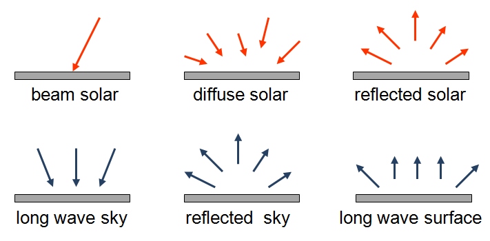
As the solar radiation passes through the atmosphere, it gets absorbed, scattered, reflected, or transmitted. All these processes result in reduction of the energy flux density. Actually, the solar flux density is reduced by about 30% compared to extraterrestrial radiation flux on a sunny day and is reduced by as much as 90% on a cloudy day. The following main losses should be noted:
- absorbed by particles and molecules in the atmosphere - 10-30%
- reflected and scattered back to space - 2-11%
- scattered to earth (direct radiation becomes diffuse) - 5-26% [Stine and Harrigan, 1986]
As a result, the direct radiation reaching the earth surface (or a device installed on the earth surface) never exceeds 83% of the original extraterrestrial energy flux. This radiation that comes directly from the solar disk is defined as beam radiation. The scattered and reflected radiation that is sent to the earth surface from all directions (reflected from other bodies, molecules, particles, droplets, etc.) is defined as diffuse radiation. The sum of the beam and diffuse components is defined as total (or global) radiation.
It is important for us to differentiate between the beam radiation and diffuse radiation when talking about solar concentration in this lesson, because the beam radiation can be concentrated, while the diffuse radiation, in many cases, cannot. For that matter, the solar systems utilizing concentrating collectors will work best in sunny locations and may be not feasible in those with a lot of weather variability and clouds.
Only beam component of solar radiation can be effectively concentrated
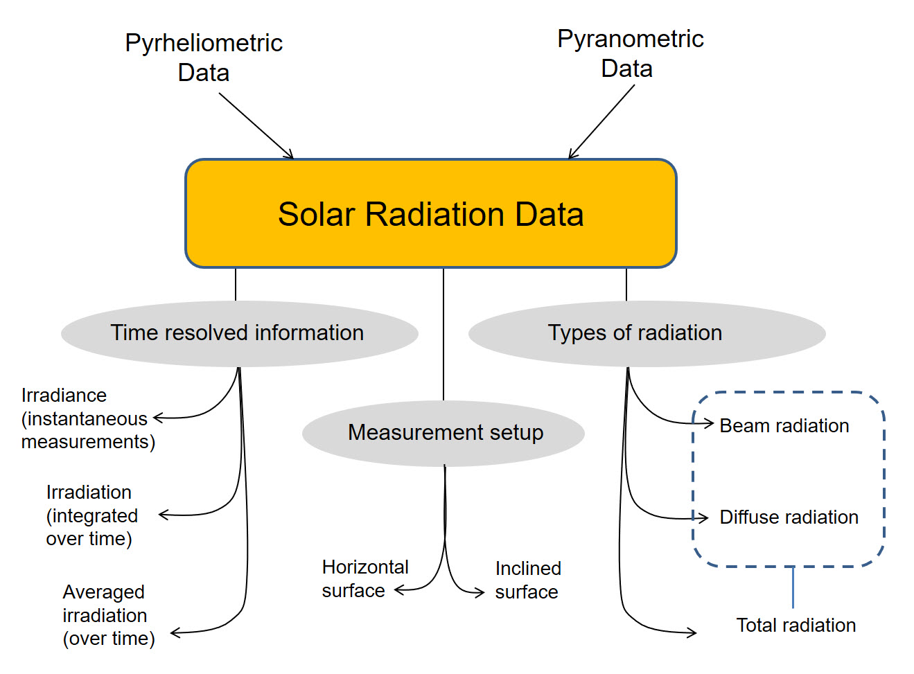
Solar Radiation Metrics
Consider the following metrics commonly used to report the solar resource (irradiance) data. These values can be determined from the field measurements or from empirical correlations.
| Metric | Definition | Data Source | Tool |
|---|---|---|---|
| DNI | Direct Normal Irradiance (W/m2) | Measured on the surface perpendicular to the beam | Pyrheliometer |
|
DHI |
Diffuse Horizontal Irradiance (W/m2) (also may be denoted DIFF) | Measured on the horizontal surface | Pyranometer (shaded) |
| GHI | Global Horizontal Irradiance (W/m2) - includes both beam and diffuse components | Measured on the horizontal surface | Pyranometer |
Theoretically, these three metrics are interrelated:
(θz = solar zenith angle)
However, in practice, field measurements may somewhat deviate from this relationship.
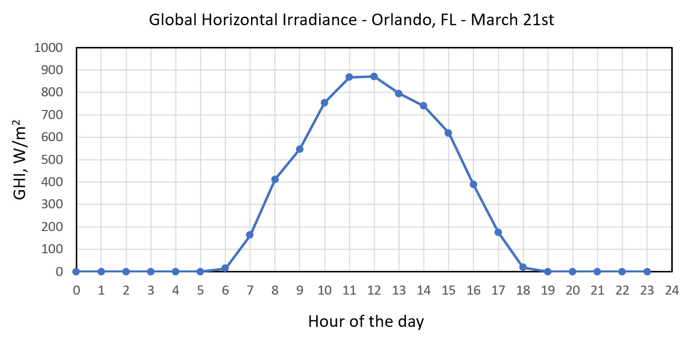
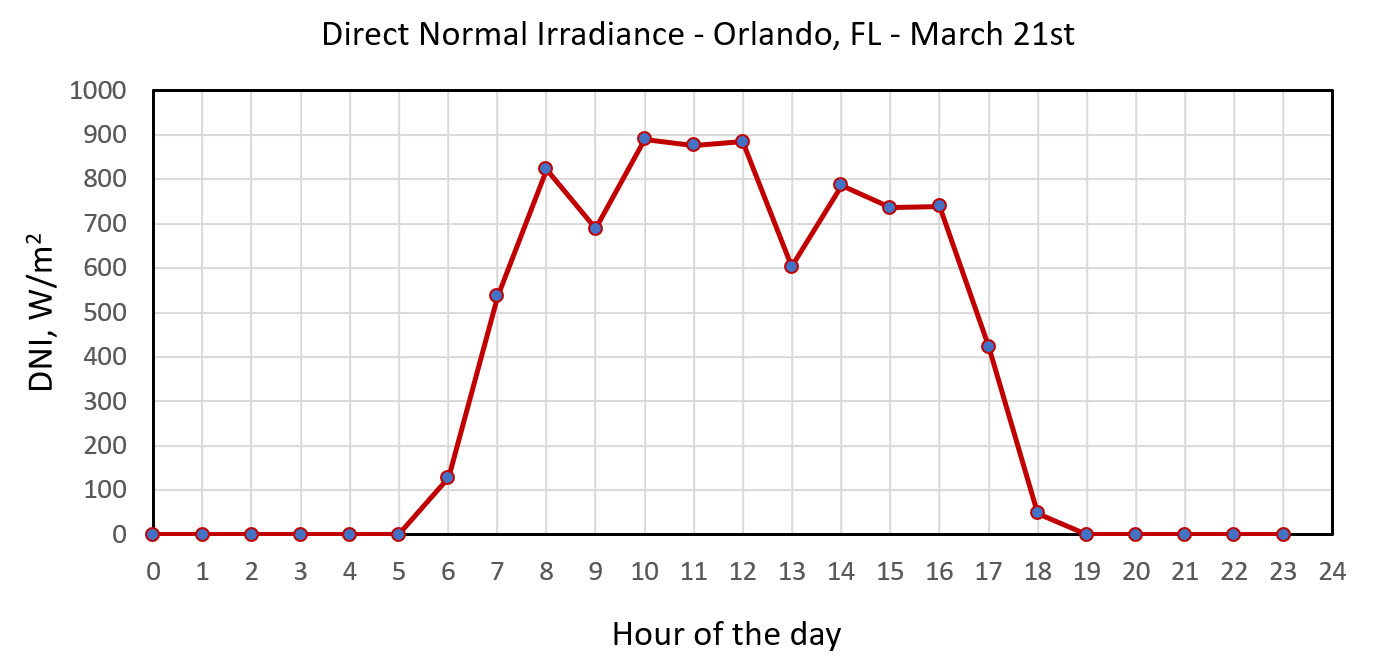
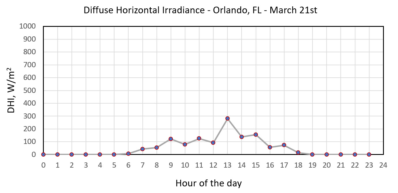
A typical solar resource data file (Typical Meteorological Year or TMY) would include all of these metrics measured for a specific location for each hour for each day in a year. Note that these values (measured in W/m2) indicate the instantaneous solar flux, which of course will vary during the day. In the morning and in the evening, the irradiance will be lower, but it will often reach its peak around solar noon. If there are clouds or other weather phenomena, the irradiance will temporarily drop.
The plots below give you an example of such variance. The GHI, DNI, and DHI data are plotted for the day of March 21st (equinox) in Orlando, FL. While it seemed to be a relatively sunny day (the beam component evidently dominates over diffuse, reaching ~900 W/m2), there are some minor interruptions (possibly from clouds) to this profile.
The TMY files with all these metrics given for each day for different locations around the globe are publicly available from the NSRDB database.
Try This!
Here is how you can download a solar resource file from the NSRDB Database. You can use this file in System Adviser Model (SAM) simulations or just for retrieving irradiance values for your locale for any specific day in a year.
Video: Download Weather File from the NSRDB (4:50)
Intro
In this video, I'll demonstrate how to download a weather file from the National Solar Radiation database to use in SAM.
Download Weather File
The first thing I'll want to do is to open a web browser and go to nsrdb dot nrel dot gov, and then click the blue nsrdb viewer button. Then I'll click download and, starting on the intro tab, I will type an email address. You'll want to type your own email address here and then click get started. Then on the data and location tab it asks me to select a layer. I want to download TMY data. So, I'm going to choose the USA and America's typical meteorological year data option, but you could choose any of the other ones.
And then for the location, I'm going to enter coordinates manually. So, I'll choose this option, and then I'm going to use Google Maps to find the latitude and longitude of my location. So, let's say I'm downloading a file for the NREL visitor center. I'll right click on the map here and read the values from here. So, it's 39.7 and -105.2 and then I'll click next.
That takes me to the attributes tab, where I select attributes. By default, the attributes that SAM wants are already checked, but I could check these additional attributes if I wanted that data in my weather file. SAM would just ignore those. And then for select year I'm going to choose the most recent TMY data set. So I'll choose TMY 2020.
I could choose more than one data set to choose to download more than one file. And then for the interval, I want 60 minutes data. That's all that's available. So I'll select that and then SAM needs the weather data to be in local time so I want to make sure that convert UTC to local time is checked. Then I click download and that should result in an email being sent. If I go off screen here and look at my email, I see an email from no reply at NREL dot gov.
It has the subject NREL data download ready. That might be in your junk folder, so you might want to check there. If you don't see the email and the email contains a link that I'll click to download the weather file.
Add Weather File to SAM
And if I look in my downloads folder, I'll see that there's this file. The zip file with a number for a file name. So, in order to use this data in SAM, I'm going to need to get the csv file that's inside the zip archive and put it in a folder on my computer and then tell SAM where that folder is. So, let's get that csv file out of this file out of the zip archive. I can extract it or just in windows, I can just copy it from the zip archive and paste it into another folder. I'm going to create a folder on my desktop.
I could put this folder anywhere on my computer, and then I'll paste the csv file here and then now I need to go to SAM. So, in SAM, I'll go to the location and resource page and add the folder. So, I'll click add remove weather file folders and then add and navigate to the folder that I just created which is on desktop and SRDB data, select folder and then click ok. So, what Sam does is it looks in that folder for any CSV files and scans them to see if they're a valid weather file. If the weather file is valid, then it adds it to the solar resource library, and then you can just select it in the solar resource library, check the data, and use it for your simulation.
Bookmark this video. It will help you get the data you need for SAM assignments later in this course or for your project.
Solar Maps
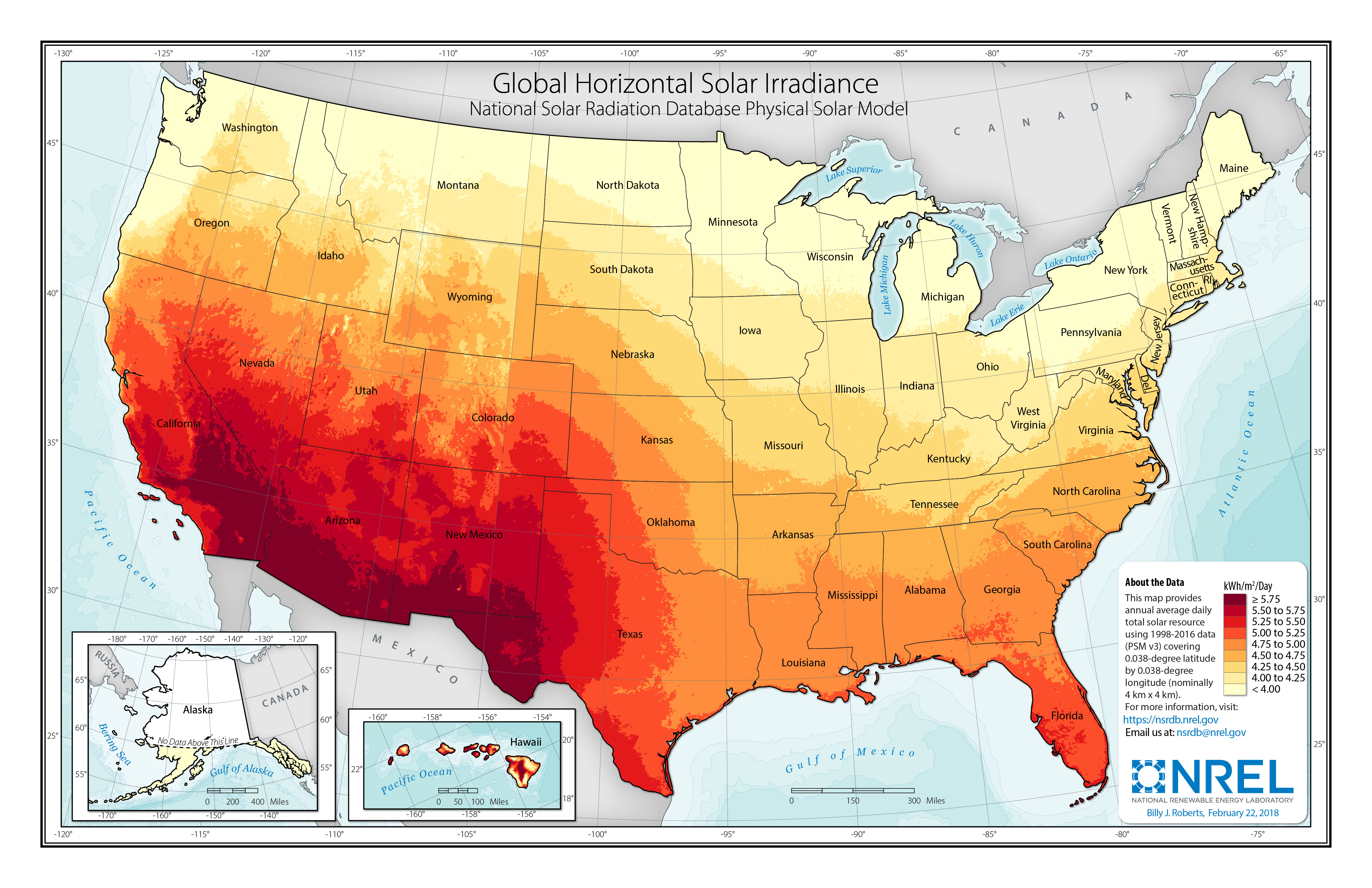
The GHI data are also used to generate solar resource maps. However, the instantaneous values of global irradiance are not best for mapping due to their continuous variability. Instead, GHI are integrated to determine the daily average irradiation (total energy from the sky).
Look again at the GHI plot (blue curve above) – essentially, this total daily energy will be equal to the area under the irradiance curve! This total daily irradiation value (measured in kWh/m2/day) can be better related to the total energy converted and delivered by your solar system. In a practical sense, it is a more intuitive metric to map.
Also, let’s not forget the seasonal variations. The solar daily irradiation will be understandably higher during summer months and lower during winter months. Hence, the map below is based on the annual average values of daily irradiation.
Probing Question
Let’s take another look at the daily irradiance profile for Central Florida (blue curve): by integrating the GHI over the hours of the day, we can estimate the daily total irradiation at ~6.37 kWh/m2/day.
Now let’s look at the solar resource map. The Central Florida location would correspond to only 5-5.25 kWh/m2/day.
What is the reason for this difference? Which value should we consider for modeling our solar system performance?
Short-Wave and Long-Wave
Short-wave radiation, in the wavelength range from 0.3 to 3 μm, comes directly from the sun. It includes both beam and diffuse components.
Long-wave radiation, with wavelength 3 μm or longer, originates from the sources at near-ambient temperatures - atmosphere, earth surface, light collectors, other bodies.
The solar radiation reaching the earth is highly variable and depends on the state of the atmosphere at a specific locale. Two atmospheric processes can significantly affect the incident irradiation: scattering and absorption.
Scattering is caused by interaction of the radiation with molecules, water, and dust particles in the air. How much light is scattered depends on the number of particles in the atmosphere, particle size, and the total air mass the radiation comes through.
Absorption occurs upon interaction of the radiation with certain molecules, such as ozone (absorption of short-wave radiation - ultraviolet), water vapor, and carbon dioxide (absorption of long-wave radiation - infrared).
Due to these processes, out of the whole spectrum of solar radiation, only a small portion reaches the earth's surface. Thus, most x-rays and other short-wave radiation is absorbed by atmospheric components in the ionosphere, ultraviolet is absorbed by ozone, and not-so abundant long-wave radiation is absorbed by CO2. As a result, the main wavelength range to be considered for solar applications is from 0.29 to 2.5 μm [Duffie and Beckman, 2013].
Transmittance
The effects of radiation scattering and absorption vary with the time of the day (due to the change of the air mass through which the beam passes through) and seasonally with the time of the year. Hence, the actual beam irradiance on the surface can be empirically estimated using a set of atmospheric parameters and Sun-Earth geometry.
Hottel’s method (Hottel 1976) describes the beam radiation transmitted through the atmosphere under the “clear-sky” conditions using atmospheric transmittance coefficient.
where Gbn is the beam irradiance normal to the receiving surface, Gon is the extraterrestrial irradiance (solar constant in a general case), and τb is beam transmittance.
The transmittance value can be evaluated by Hottel’s model using solar zenith angle and altitude for several different climate regimes. Or, it can be determined by direct measurement of the beam irradiance on the normal surface.
Reading Assignment
This is the description of the Hottel’s method for the calculation of the atmospheric transmittance. Please take a look.
Book chapter: Duffie, J.A. Beckman, W., Solar Engineering of Thermal Processes, Chapter 2 pp. 68-70 [18].
This section also provides a couple of examples that show how to estimate transmittance for a specific locale. This material will be helpful for solving problem #4 in your homework.
Instruments
The amount of solar radiation on the earth's surface can be instrumentally measured, and precise measurements are important for providing background solar data for solar energy conversion applications.
Described below are the most important types of instruments to measure solar radiation:
- Pyrheliometer is used to measure direct beam radiation at normal incidence. There are different types of pyrheliometers. According to Duffie and Beckman (2013), Abbot silver disc pyrheliometer and Angstrom compensation pyrheliometer are important primary standard instruments. Eppley normal incidence pyrheliometer (NIP) is a common instrument used for practical measurements in the US, and Kipp and Zonen actinometer is widely used in Europe. Both of these instruments are calibrated against the primary standard methods.
Based on their design, the above listed instruments measure the beam radiation coming from the sun and a small portion of the sky around the sun. Based on the experimental studies involving various pyrheliometer design, the contribution of the circumsolar sky to the beam is relatively negligible on a sunny day with clear skies. However, a hazy sky or a uniform thin cloud cover redistributes the radiation so that the contribution of the circumsolar sky to the measurement may become more significant.
-
Pyranometer is used to measure total hemispherical radiation - beam plus diffuse - on a horizontal surface. If shaded, a pyranometer measures diffuse radiation. Most of solar resource data come from pyranometers. The total irradiance (W/m2) measured on a horizontal surface by a pyranometer is expressed as follows:
\[{I_{tot}} = {I_{beam}}\cos \theta + {I_{diff}}\] (2.1) where θ is the zenith angle (i.e., angle between the incident ray and the normal to the horizontal instrument plane.
Examples of pyranometers are Eppley 180o or Eppley black-and-white pyranometers in the US and Moll-Gorczynsky pyranometer in Europe. These instruments are usually calibrated against standard pyrheliometers. There are pyranometers with thermocouple detectors and with photovoltaic detectors. The detectors ideally should be independent on the wavelength of the solar spectrum and angle of incidence. Pyranometers are also used to measure solar radiation on inclined surfaces, which is important for estimating input to collectors. Calibration of pyranometers depends on the inclination angle, so experimental data are needed to interpret the measurements.
- Photoelectric sunshine recorder. The natural solar radiation is notoriously intermittent and varying in intensity. The most potent radiation that creates the highest potential for concentration and conversion is the bright sunshine, which has a large beam component. The duration of the bright sunshine at a locale is measured, for example, by a photoelectric sunshine recorder. The device has two selenium photovoltaic cells, one of which is shaded, and the other is exposed to the available solar radiation. When there is no beam radiation, the signal output from both cells is similar, while in bright sunshine, signal difference between the two cells is maximized. This technique can be used to monitor the bright sunshine hours.
A more detailed explanation of how these instruments work and what kind of data is obtained from those measurements is available in the following Duffie and Beckman (2013) book, referred below. Please spend some time acquiring basic knowledge on solar resource data. For everyone who took EME 810 and is more or less familiar with this topic, this still may be a useful refresher.
Solar radiation data collected through the above-mentioned instrumental methods provide the basis for development of any solar projects. We can summarize the types of solar resource data as follows:
Before moving on, please work through the following self-check questions to assess your learning:
Check Your Understanding - Questions 1-3
Check Your Understanding - Question 4
Can you write down the value of the solar constant? What is its units and meaning?
Check Your Understanding - Question 5
How would you estimate the beam radiation intensity on the earth's surface based on the solar constant and transmittance of the atmosphere of 0.5 at a certain location? Type in the number here:
Supplemental reading
NREL Report: Stoffel et al. (2010): Concentrating Solar Power: Best Practices Handbook for the Collection and Use of Solar Resource Data [19], NREL/TP-550-47465.
Book Chapter: Duffie, J.A. Beckman, W., Solar Engineering of Thermal Processes [20], Chapter 2.
Assuming that you have already learned about solar resource in your prerequisite courses, I suggest these readings as optional resources if you are inclined to dive deeper into this topic.
2.2 Types and Elements of Concentrating Collectors
2.2 Types and Elements of Concentrating Collectors
Any general setup for the conversion of the solar energy includes a receiver - a device that is able to convert the solar radiation into a different kind of energy. This can be either a heat absorber (to harvest thermal energy) or a photovoltaic cell (to convert light to electric energy). In the first case, the thermal radiation is absorbed to heat a medium (fluid), which transfers that absorbed energy to a generator. In the second case, light causes a photovoltaic effect in the material of the solar cell, which generates electric current. In both of these situations, the amount of energy available for the conversion is only as much as the solar source supplies per unit area of the converter.
If we need more energy for use, we have two options. The first option is to increase the system scale (for example by increasing the number of receivers). In other words, we have to expand the plant area, which would involve additional cost for construction, service, maintenance, and may require additional land, more materials, etc. It has been done to some extent, but sometimes it is not a sufficient measure to meet the energy demands, especially if land area is a constraint. The second option is to concentrate the radiation flux. This can be achieved by placing a concentrator (usually some kind of optical device) between the light source (sun) and the receiver. By common terminology, a solar collector is a sunlight processing system that includes a concentrator and a receiver in its setup; it is also characterized by aperture - the cross sectional area through which sunlight accesses the system.
The most common concentrators are reflectors (mirrors) and refractors (lenses), which modify and redirect the incident sunlight beam. The design of the concentrating optics varies. Some of the examples of concentrating collectors, which involve diversely shaped mirrors, are shown in Figure 2.3, as they applied to the solar-to-thermal energy conversion.
The process of light concentration implies first of all that the energy flux is increased due to confining it to a smaller area. This brings several important benefits:
- reaching higher temperatures for heat collectors;
- heat losses from the surface of the receiver are decreased because the receiving area is decreased;
- higher energy conversion rate can be achieved over smaller area.
Concentration implies confining solar radiation flux to a smaller area compared to original aperture.
There are two major classes of solar concentrators: imaging and non-imaging. Imaging concentrators are called imaging because they produce an optical image of the sun on the receiver. Non-imaging concentrators do not produce such an image, but rather disperse the light from the sun over the whole area of the receiver. Non-imaging concentrators have relatively low concentration ratio (<10) compared to the imaging concentrators.
All of the optical tools designed for manipulating sunlight for the purpose of its concentration and efficient utilization are based on the fundamental optics principles, which you may remember from physics courses. In case you need to refresh your knowledge of those fundamentals before we study the light concentration principles, please refer to the following reading and video:
Reading and Video Assignment
Web article: "Light Reflection and Refraction [21]", Science Primer 2011-2013.
This webpage has a good explanatory video, which I suggest you to watch.
Out of the different types of concentrators listed above, mainly the following four technologies have been adopted for use in the utility scale CSP facilities [Mendelsohn et al., 2012]:
- Parabolic trough
- Solar tower
- Parabolic dish
- Linear Fresnel reflector
All of these are imaging concentrators which allow relatively high concentration temperatures: about 400 oC for parabolic troughs, up to 650 oC for Stirling dishes, and above 1000 oC for solar power towers. Just for comparison, non-imaging concentrators would work maximum up to 200 oC. These technologies will be introduced in more detail in Lessons 7 and 8 of this course.
There are also developments for non-imaging compound parabolic collectors (CPC) to be used at the utility scale for low-temperature applications [Baig et al., 2009], but this technology is not as widespread due to its moderate concentrating capabilities. Its flexibility with respect to using non-beam radiation and more relaxed technical requirements to positioning of concentrators are still attractive, so this technology will be also included in our consideration.
Concentrating photovoltaics is another technology class that uses concentrated light, but those devices will be covered separately in Lessons 5 and 6 of this course.
2.3 Concentration Ratio
2.3 Concentration Ratio
The light concentration process is typically characterized by the concentration ratio (C). By physical meaning, the concentration ratio is the factor by which the incident energy flux (Io) is optically enhanced on the receiving surface (Ir) - see Figure 2.4. So, confining the available energy coming through a chosen aperture to a smaller area on the receiver, we should be able to increase the flux.
| (2.2) |
In the above equation, Cgeo is called the geometric concentration ratio. It is easy to use, as the areas of the devices are known, although it is adequate only when the radiation flux is uniform over the aperture and over the receiver. Also, please note that for some imaging concentrators, the area of the available receiver surface can be different from the area of the image produced by the concentrator on the receiver. So, if the image does not cover the entire surface of the receiver, we need to use the image area to estimate the concentration ratio.
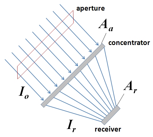
The concentration ratio can also be represented by the energy flux ratio at the aperture and at the receiver. In this case, it is termed optical concentration ratio Copt (or flux concentration ratio) and can be directly applied to thermal calculations.
| (2.3) |
In case the ambient energy flux over the aperture (insolation) and over the receiver (irradiance) is uniform, the geometric and optical concentration ratios are equal (Cgeo = Copt).
The concentration ratios are important metrics used to characterize and rank optical concentrators. Next, we will look at several examples of concentrator designs and see what values of concentration ratios they can provide.
There is a theoretical limit to solar concentration. For circular concentrators - 45,000, and for linear concentrators - 212, based on the geometrical considerations; however, these limits may be unreachable by real systems because of non-idealities and losses. If you are interested in the analytical estimation of the concentration limits, refer to Duffie and Beckman's (2013) book (p.325) for more details.
In general sunlight, concentration systems are roughly classified into: low concentration range (C<10), medium concentration range (10<C<100), and high concentration range (C>100). However, only some of the systems provide uniform concentrated light flux (e.g., V-troughs or pyramidal plane reflectors) and can be characterized by a single concentration ratio. Many systems with curved reflecting surfaces (e.g., conical, parabolic, spherical) create a distribution of flux density over the receiver and would rather be characterized by a variable C over the receiver width. In that case, a local concentration ratio (Cl) is the main parameter to characterize the performance of the ideal concentrator:
|
(2.4) |
where I(y) is determined for any local position y from the center of the produced image, and Iap is the intensity of the incident radiation at the aperture.
In many typical cases of imaging concentrators, the reflectance of the surface (ρ), i.e., the fraction of light radiation reflected from the surface compared to the total incident radiation, is also taken into account. Then the local intensity of the concentrated light, I(y), can be described as follows:
|
(2.5) |
Further, in this lesson, we will study some examples that use this equation to estimate energy distribution within a concentrated image on the receiver. It would be better to have a specific type of concentrator to apply these concepts. Please read through the following text to enforce your understanding of the concentration ratios.
Reading Assignment
Book chapter: Duffie, J.A. Beckman, W., Solar Engineering of Thermal Processes [20], Chapter 7: introduction through Section 7.2. pp. 322-327.
The above-referenced sections of the book in part repeat some of the material given here, but may give you more extensive commentary on the basics and probably provide deeper insight how concentration ratio is influenced by other parameters of the system.
After you have completed the above reading assignment, please answer a few self-check questions below.
Check Your Understanding - Question 1
Check Your Understanding - Question 2
When are the optical and geometric concentration ratios equal?
Check Your Understanding - Question 3
Check Your Understanding - Question 4
If the radiation intensity is distributed unevenly within an image produced by an imaging collector, what parameter is typically used to characterize the concentration performance?
Check Your Understanding - Question 5
2.4 Concentration with a Parabolic Reflector
2.4 Concentration with a Parabolic Reflector
Parabolic geometry is the basis for such concentrating solar power (CSP) technologies as troughs or dishes. Parabolic trough is also considered one of the most mature and most commercially proven technologies in the utility scale CSP facilities (Mendelsohn et al., 2012), so we will look at the physical principles of parabolic concentrators in some more detail.
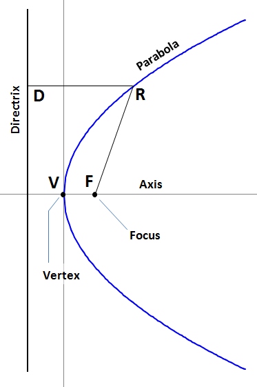
Geometrically, a parabola is a locus of points that lie on equal distance from a line (directrix) and a point (focus) - see Figure 2.6. For each point of the parabola, DR = FR. The distance VF between the vertex and focus of the parabola is the focal distance (f). The line perpendicular to the directrix that passes through the focus is the axis of the parabola; the axis divides the parabola into two parts that are symmetrical.
With origin at its vertex, and the axis of the parabola taken as x-axis, a parabola is described by the equation:
| (2.5) |
where f is the focal length.
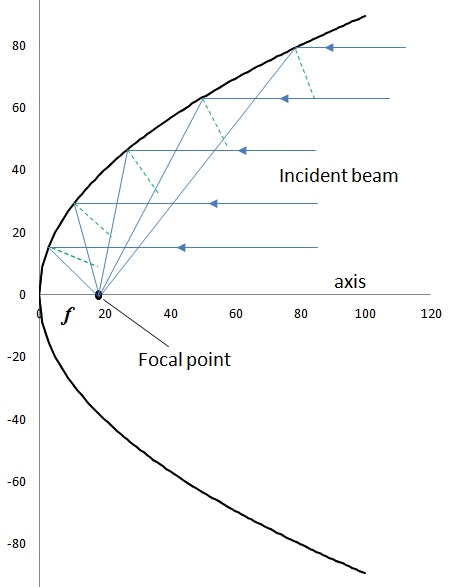
By definition of the focal point of the parabola, all incoming rays parallel to the axis of the parabola are reflected through the focus. This provides an opportunity for light concentration by using parabolic surfaces. If we assume that solar light arrives to the surface as essentially parallel rays, and apply the Snell's law (the angle of reflection equals the angle of incidence), we can assign the focal point as an ideal location for the receiver (Figure 2.7).
Solar applications deal with a parabola of a finite height (Figure 2.8). The design of the parabolic reflector takes into account the available aperture size (a), focus location (f - i.e., where receiver would be placed), and height of the reflector (h). These parameters are interrelated via the equation (Stine and Harrigan, 1986):
| (2.6) |
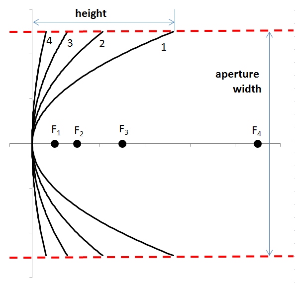
This figure above shows that the flatter the reflecting surface, the longer the focal length. The "flatness" of the shape of a finite parabola is typically characterized by the rim angle ( ). When rim angle increases (within the same aperture), the parabola becomes more curved, and the focal distance shortens.
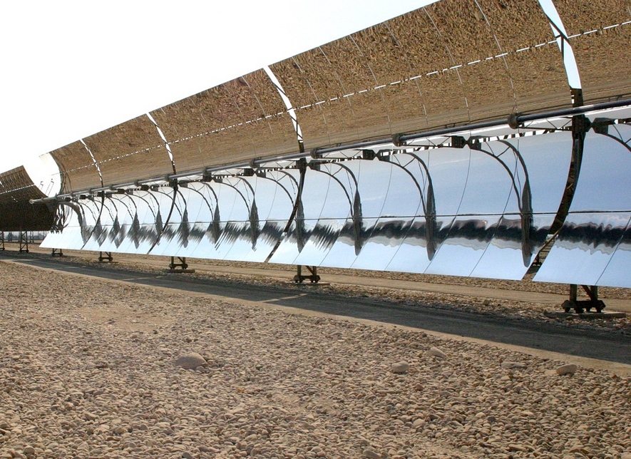
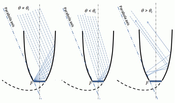
Parabolic trough (Figure 2.9) is a typical example of an imaging concentrator that utilizes the geometric relationships discussed above. Parabolic trough is one of the most widely implemented technologies for sunlight concentration at the utility scale. This type of collectors relies on sun tracking to ensure that the beam radiation is directed parallel to the parabolic axis.
A parabolic mirror produces an image of the sun on the surface of the receiver, so the receiver size needs to be matched to the image size. Consider Figure 2.10, which illustrates this idea. Since the sun is not really a point source, solar beam incident on the reflector is represented as a cone with an angular width 0.53o (so the half-angle between the cone axis and its side is 0.267o). Being reflected at a point on the parabolic surface, the beam hits the focal plane, where it produces an image of a certain dimension, centered around the focal point. The diameter of the cylindrical receiver (D), which would intercept the entire reflected image can be theoretically calculated using aperture width (a), and rim angle ( ) as follows (Duffie and Beckman, 2013):
| (2.7) |
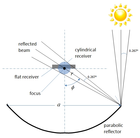
For the linear receiver, the width of the image (W) produced on the focal plane can be determined as follows:
| (2.8) |
The equations presented here can be used to estimate the size of the reflected light image on the receiver for different shapes of parabolic reflectors. The formulas include a as a chosen aperture of the reflector (width of the trough), and ( ) as a measure of parabolic curvature. Note that these are the minimal theoretical dimensions of the reflected image that would be produced by the ideal parabolic mirror that is perfectly aligned. If there are any flaws in the mirror surface or trueness of the angle, additional spreading of the image may occur. If you are interested in more explanation of how these formulas were derived, please refer to Duffie and Beckman, 2013 book (Section 7.9)
The above-described geometrical concepts apply to the cross-section of a parabolic reflector. In reality, the reflector itself is a three-dimensional shape, i.e., a parabolic cylinder with a finite length (l). So, the cone-shaped ray reflected at a point on the surface of a parabolic reflector will produce an ellipse-shaped image on the focal plane. We can see that as the reflection point is moved away from the vertex towards the rim, the ellipse transforms from a circular to a more and more elongated shape (because the cone would be sectioned by the focal plane at greater and greater angle - Figure 2.11).
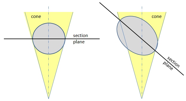
Knowing the angular width of the cone, the dimensions of the ellipse image can be theoretically derived and presented as a function of (angle of deviation from the parabola axis). Below are the equations describing the length of the minor and major axes of the ellipse.
| (2.9) |
| (2.10) |
where r is the distance between the focus and reflection point (local radius) on the parabolic mirror (r=f at the vertex); is the angle between the parabola axis and the ray, and 0.267o is the half-angle of the ray cone width.
The superposition of these individual ellipses produced by each element of the reflector form the total image, which is not uniform, but rather has a distribution of light intensity. The focal length (which is related to the rim angle of the reflector) is responsible for image size, while the aperture is responsible for the total amount of energy concentrated by a collector. So, the total image intensity (brightness) at the receiver should be a function of a/f. The image brightness essentially reflects the energy flux concentration:
Energy flux concentration ~ a/f
The larger the aperture, the more energy is concentrated within a certain image size. The smaller the focal length, the smaller the image size within which the energy is concentrated.
The distribution of intensity of the energy flux within the concentrated image may have a profile similar to Figure 2.5. Different models have been applied to quantify that profile. For example, one of the approaches is called nonuniform solar disk, which suggests that the sunlight intensity coming out of the center of the solar disk is higher than that coming from its edges [Evans, 1977]. Without going into too much detail of this model, we can use the diagrams presented in the book by Duffie and Beckman (2013), which allow connecting various parameters of a parabolic concentrator with the local intensity on the receiver.
Please refer to the following reading to study the tools for image analysis via the nonuniform solar disk model, and be sure to study the example presented therein, which is very helpful.
Reading Assignment
Book chapter: Duffie, J.A. Beckman, W., Solar Engineering of Thermal Processes [20], Chapter 7: the introduction through Section 7.10. pp. 354-358.
The main goal for this assignment is to understand how to estimate concentrated image parameters using model diagrams 7.10.1, 7.10.2, and 7.10.3.
Please answer the following quick questions to check your understanding of some of the basic points in this section. The parabola cheatsheet [23]presents a useful summary for your notes.
Check Your Understanding - Questions 1-2
Check Your Understanding - Question 3
What is the key optical property of a parabolic mirror that allows for high ratio of light concentration?
Check Your Understanding - Questions 4-5
2.5 CPC Collectors - Concentration of Diffuse Radiation
2.5 CPC Collectors - Concentration of Diffuse Radiation
The compound parabolic concentrators (CPC) are typical representatives of non-imaging concentrators, which are capable of collecting all available radiation - both beam and diffuse - and directing it to the receiver. These concentrators do not have such strict requirements for the incidence angle as the parabolic troughs have, which makes them attractive from the point of view of system simplicity and flexibility. Like parabolic and other shapes, CPC concentrators can be applied in both linear (troughs) and three-dimensional (parabolocylinder) versions. The same as in "pure" parabola case, troughs are most widespread and useful for this type of concentrator.
The geometry of a CPC collector is demonstrated in Figure 2.12. If we consider a CPC trough, this diagram represents its cross-section. Each side of the shape is a parabola, and each of the parabolas has its focus at the lower edge of the other parabola (e.g., F is the focus of the right-hand parabola in Figure 2.12). Each parabola axis is tilted relative to the axis of the CPC shape. One of its key parameters is acceptance half-angle (), which is the angle between the axis of the collector and the line connecting the focus of one of the parabolas with the opposite edge of the aperture. The collector is designed in such a way that each ray coming into the CPC aperture at an angle smaller that reaches the receiver; if this angle is greater than , the ray will return (Figure 2.13). The relationship between the size of the aperture (2a), the size of the receiver (2a') and the acceptance half-angle is expressed through the following equation:
| (2.11) |
Knowing that the geometric concentration ratio is the quotient of the aperture area to the receiver area (see Section 2.3), for a linear CPC concentrator, we can obtain the relationship between the concentration ratio and the acceptance angle:
| (2.12) |
One large parabolic mirror with a second mirror sitting tangent to the parabolic axis with an end at mirror #1’s focus. The distance between the two upper ends of the parabolas is labeled aperture (2a) and the bottom two ends is labeled receiver. Dashed lines connect one top end to the opposite bottom end. The angle between their y intercept, y-axis and upper tip represents the acceptance half-angle.
There are some other useful expressions that describe the design of CPC concentrators. The following equations relate the focal distance of the side parabola (f) to the acceptance angle, receiver size, and height of the collector (Duffie and Beckman, 2013):
| (2.13) |
| (2.14) |
Please complete the following reading to further explore the work principle of CPC concentrators.
Reading Assignment
Book chapter: Duffie, J.A. Beckman, W., Solar Engineering of Thermal Processes [20], Chapter 7: Sections 7.6 and 7.7 - pp. 337-349. This book is available online through the PSU Library system and can also be accessed through e-reserves (via the Library Resources tab).
Section 7.6. of this book covers the fundamental optical principles of CPC collectors and also considers particular cases of truncated collector. Some practical examples are also presented. Section 7.7. talks about the orientation of CPC collectors. While CPC technology does not require continuous tracking, proper orientation with respect to the sun position is crucial to maximize absorbed radiation. The theoretical material in this section is also supported by practical examples.
The following self-check questions will help you to test check your learning of the principles of CPC collectors:
Check Your Understanding - Questions 1-4
Check Your Understanding - Question 5
Can you calculate what would be the acceptance angle for a CPC collector with side parabola focal distance f=20 cm and width of the receiver 2a'=30 cm?
Summary and Activities
Summary and Activities
Lesson 2 covers fundamental principles of light concentration that are important for a number of solar energy conversion technologies - both thermal and photovoltaic conversion. The general scheme of the solar energy concentration is this:
Input solar energy flux ⇒ Optical concentration device ⇒ Output concentrated solar energy flux
We touched upon each of these stages. First, we looked at the available solar radiation at the earth surface - the input we start with. Then, we considered a few techniques that concentrate the available flux, confining it to a smaller area. Finally, we looked at the output and its characteristics. Theoretical and empirical laws presented in the readings provide you with the background for estimating such parameters as concentration ratio and output energy density. Most of the theoretical considerations presented here are made for ideal systems. In reality, you can expect that imperfect optics will require additional corrections for non-ideality and losses. Limitations and advantages of specific concentrating technologies will be considered in further lessons, separately for CSP and photovoltaic systems.
After you have covered the assigned materials for this lesson, please complete the following assignments:
| Type | Description/Instructions |
|---|---|
| Reading Quiz | Please complete the Lesson 2 Reading Quiz. |
| Written Assignment | Lesson 2 Activity: Light Concentration Problem Set
|
References for Lesson 2
Stine, W.B. and Harrigan, R.W., Solar Energy Systems Design, John Wiley and Sons, Inc., 1986.
Duffie, J.A. and Beckman, W.A., Solar Engineering of Thermal Processes, 4th Ed., John Wiley and Sons, 2013.
Mendelsohn, M., Lowder, T., and Canavan, B., Utility-Scale Concentrating Solar Power and Photovoltaics Projects: A Technology and Market Overview 2012, Technical Report
NREL/TP-6A20-51137 [24], April 2012
Baig, M.N., Asad, K.D., and Tariq, A., CPC-Trough—Compound Parabolic Collector for Cost-Efficient Low-Temperature Applications, Proceedings of ISES World Congress 2007 (Vol. I – Vol. V) pp. 603-607 (2009).
Evans, D.L., On the performance of cylindrical parabolic solar concentrators with flat absorbers, Solar Energy, 19, 279 (1977).
IPS - Radio and Space Services, [25] Australian Government (accessed Oct. 2014).
Hottel, H.C., A Simple Model for Estimating the Transmittance of Direct Solar Radiation Through Clear Atmospheres, Solar Energy, 18, 129 (1976).
Lesson 3: Tracking Systems
Overview
Overview
This lesson will introduce the concept of sun tracking and will discuss how it can improve the performance of solar energy systems. The sun is a light source that is not fixed, but rather is constantly moving relative to a solar receiver. This leads to significant variability of the available radiation and, as a result, variability of power output and efficiency of a solar energy conversion system. The idea of sun tracking was developed in attempt to mitigate that variability to some extent and in pursuit of higher efficiency and extending the solar power production over the course of the day. Tracking technology is more often associated with utility scale solar plants rather than small residential systems. Some examples of tracking include single-axis and two-axis tracking of PV panels, moving heliostats in solar tower thermal plants, variable tilt parabolic trough systems, and Stirling dish concentrators - systems whose operation heavily relies on the accuracy of tracking. In this lesson, we will first discuss when tracking is a viable idea, and what systems can benefit from it. Then, we will study the geometry of the solar motion through the sky and define the parameters that characterize the position of the sun relative to a solar receiver at a certain location and time. This background would be important in understanding any tracking algorithms. Some examples and activities within this lesson will involve geometric calculations that will help you to better understand how this technology works.
Learning Objectives
By the end of this lesson, you should be able to:
- define the main parameters of the solar motion;
- explain the types of tracking systems and principles of their operation;
- calculate the position of the sun relative to the receiving surface at a locale at a particular time.
Readings
Kaligirou, A, Solar Energy Engineering, Chapter 2: Environmental Characteristics.
Brownson, J.R.S., Solar Energy Conversion Systems, Chapter 7. Applying the Angles to Shadows and Tracking, pp. 192-196.
Both books are available for reading online through the Penn State Library system. See the "Library Resources" / E-Reserves tab in Canvas.
3.1. Why tracking?
3.1. Why tracking?
Solar tracking is a technology for orienting a solar collector, reflector, or photovoltaic panel towards the sun. As the sun moves across the sky, a tracking device makes sure that the solar collector automatically follows and maintains the optimum angle to receive the most of the solar radiation. Some solar concentrators hugely benefit from tracking, while some others do not. So, the tracking systems can be added with additional cost and certain trade-offs in system design only when it pays off.
The required accuracy of tracking varies with application. For example, concentrators, especially in solar cell applications, require a high degree of accuracy to ensure that the concentrated sunlight is directed precisely to the solar conversion element. Tracking the sun from east in the morning to west in the evening can increase the efficiency of a solar panel up to 45%, according to some manufacturers [Linak [26]]. Precise tracking of the sun is achieved through systems with single or dual axis tracking.
Watch this introductory video (5:33), which provides an illustration to the benefits of sun tracking:
DEGERenergie - Solar Tracking Systems (5:33)
NARRATOR: During the last decade, photovoltaics have become an important source of energy. DEGERenergie has been the global pioneer for solar tracking systems, optimizing the efficiency of renewable energy for more than 12 years. DEGERenergie has been providing advanced technology to increase efficiency of solar plants. And, while having set the standard of today, DEGERenergie has new visions, ideas, and solutions which stretch beyond tomorrow.
MICHAEL HECK: Located in Germany, DEGERenergie is the leading manufacturers of the largest product portfolio worldwide for single and dual access solar attracting systems. As the market leader for solar power plants, with over 35,000 star systems worldwide, we offer a German technology product with the best price-performance ratio in the business.
NARRATOR: The Fraunhofer Institute for Solar Energy Systems calculated a 27% higher output of astronomically controlled systems compared to fixed systems. Spanish solar farm operator Picon de Solar reviewed its revenues of the last few years and discovered that they had achieved a 46% higher yield using DEGER trackers than with a comparable fixed system.
MICHAEL HECK: We have been consistently developing new ideas and concepts for the optimum use of solar energy through solar module tracking.
NARRATOR: DEGERenergie develops, produces, and provides individual service for intelligent solar tracking systems, energizing the global photovoltaic market.
ANDREAS SCHWEDHELM: The heart of this technology is a sensor, which is called the DEGERconecter. The advantage of using this technology is that we can also incorporate different weather conditions. For example, the eye of cloud effect, complete overcast days or also reflections, for example, if there is snow on the ground.
NARRATOR: All DEGER trackers use the patented maximum light detection technology, MLD. Unlike other systems, the DEGERconecter measures which direction most of the light is actually coming from. In doing so, each DEGER tracker finds its own ideal position and uses reflections to raise its output. In a similar way, the DEGERconecter takes the eye of cloud effect into account and, even on completely overcast days, each DEGER tracker moves individually into an ideal position for maximum yield. Within DEGER trackers there is no need for a computer that could crash, no need for calibration or extra wiring that costs money. The simple and individual control of a DEGER tracker provides for a calibration and maintenance-free long-term availability, and guarantees a sustainable operation, even with changing soil conditions. The optimized energy output of DEGER trackers will save an investor a 25% higher expenditure than equivalent fixed systems. Investing in DEGER trackers, customers will realize a profitable internal rate of return. DEGER's systems are guaranteed to have a good future. On average, the energy recovery of DEGER systems is complete after three years, including concrete, steel, and wiring. All steel and concrete parts are completely recyclable. DEGERenergie is an innovative technology with higher yields, low maintenance cost and optimal internal rate of return, emission-free energy production and eco-friendly manufacturing, with warranties extendable to 25 years.
MICHAEL HECK: You can't always rely on the weather, but you can count on your intelligent controlled system.
NARRATOR: DEGERenergie, not only simply brilliant, but brilliantly simple.
Systems that employ trackers
So, what types of systems should include tracking devices (a.k.a. trackers)?
First of all, the systems that specifically utilize the direct beam radiation benefit from tracking. In majority of concentrating solar power (CSP) systems, the optics accept only the beam radiation and therefore must be oriented appropriately to collect energy. Such systems will not produce power unless pointed at the sun. Tracking is required for heliostats in central receiver (solar tower) systems. CSP collectors require significant degree of accuracy of sun tracking.
In photovoltaic (PV) applications, tracking devices can be used to minimize the angle of incidence of incoming solar rays onto a PV panel. This increases the amount of energy produced per unit of installed power generating capacity. This increases the efficiency of the system and its cost-effectiveness, but, at the same time, tracking is not strictly required for regular flat panel PV as they accept both beam and diffuse radiation.
In concentrating photovoltaics (CPV), the optics requires beam radiation and therefore must be oriented appropriately to focus light on the PV collector to maximize the energy converted. CPV modules that concentrate in one dimension must be tracked normal to the sun in one axis. CPV modules that concentrate in two dimensions must be tracked normal to the sun in two axes [Solar Tracker from Wikipedia.org [28]]. CPV modules require high degree of accuracy of sun tracking.
Single-axis and Dual-axis
There are many types of solar trackers, which are different in costs, design complexity, and performance. But we can distinguish two basic classes of systems:
- Single axis trackers
The single axis solar trackers can either have a horizontal or a vertical axis. The horizontal axis is used in tropical regions where the sun gets very high at noon, but the days are short. The vertical type is used in high latitudes, where the sun does not get very high, but summer days can be very long. In concentrated solar power applications, single axis trackers are used with parabolic and linear Fresnel mirror designs. - Dual axis trackers
The dual axis solar trackers have both a horizontal and a vertical axis, and thus they can track the sun's apparent motion at any location. Dual axis tracking is commonly used for CSP applications, such as solar power towers and dish (Stirling engine) systems. Dual axis tracking is extremely important in solar tower applications due to the angle errors resulting from longer distances between the mirror and the central receiver located in the tower structure.
In more detail, these types of trackers will be studied in Section 3.3. of this lesson.
Pros and Cons
With tracking incorporated in the system design, the cost of the system is understandably higher compared to fixed tilt systems. According to the US DOE report [Barbose et al., 2013], "among projects completed in 2012, the capacity-weighted average installed price in US dollars was 3.3/W for systems with crystalline modules and fixed tilt, compared to 3.6/W for crystalline systems with tracking and 3.2/W for thin-film, fixed-tilt systems." Efforts are constantly made by manufacturers to lower the cost of the tracking systems, making them less complex, more compact, reliable, and easier to maintain. In spite of the additional costs, use of trackers is often a preferred option for utility-scale installations due to the significant boost to the system performance. Figure 3-1 shows the trend of increasing use of tracking systems in the U.S. utility-scale PV installations over the 2007–2017 decade. Cumulative tracking system installation reached 79% in 2017 (meaning that only 21% of large PV installations opt not to use trackers). These data include both one-axis and dual-axis tracking systems cumulatively, however there are many more one-axis trackers deployed than dual-axis trackers.
3.2. Apparent daily path of the sun
3.2. Apparent daily path of the sun
For most solar tracking applications, we need a reasonably accurate knowledge of where the sun will be at a specific hour during each day in a year. Theory is well-developed to calculate the sun position with respect to the observation point on the earth surface, and it sets the background for design and modeling of both photovoltaic and concentrating solar power systems of various scale.
In order to discuss tracking or any other adjustments of solar receivers, it would be useful first to understand the sun's path across the sky dome. We are going to turn to the following reading, which describes the key parameters of the solar motion.
Reading Assignment
Book chapter: Kalogirou, A, Solar Energy Engineering [30], Chapter 2: "Environmental Characteristics." pp. 51-63. (See E-Reserves via the Library Resources tab.)
This reading explains a lot about the geometry of sun movement, provides the key equations and example calculations alongside with them. The objective here would be to learn how to estimate the sun position and draw its track for a particular location and time of the year.
The above materials provide the main tools for predicting the position of the sun at a location of choice at any specific time. Let us summarize a few key takeaways from this reading.
Solar Altitude and Solar Azimuth
The main parameters to determine are solar altitude (α) and solar azimuth (z). Here are the equations that are used to calculate these coordinates:
|
(3.1) |
|
(3.2) |
Let us consider an example showing how to use these equations.
Example
Calculate the solar position for Abu-Dhabi (UAE) on January 15 at 2 pm local time.
For this calculation, we will use equations (3.1) and (3.2) to find the solar altitude and solar azimuth, respectively. We will need to find the following parameters:
L - local latitude - Abu-Dhabi coordinates are: latitude 24.492o N, and longitude 54.358o E
You can use this website to get GIS data [31].
δ - declination - It is a function of the day of the year (N). For Jan 15, δ = -21.27o
as found by Eq. (2.5), Kalogirou's text.
h - hour angle - It is a function of the time of the day. For 2 pm, h = 22.04o as found by Eq. (2.9), Kalogirou's text. For calculating hour angle, you need to determine the apparent solar time (AST), which is given by Eq. (2.3) of Kalogirou's text.
You can also use this helpful resource and embedded calculator [32] to find AST. (You may want to bookmark it to use in your homework!)
Applying it to the current location, we find that AST = 13.47 hr decimal time or 1:28 pm clock time. And the hour angle will be:
h = (AST-12) x 15 = (13.47 - 12) x 15 = 22.04
Now we can plug these L, δ, and h numbers into Eq. (3.1):
sin(α) = sin (24.493o)sin(-21.27o) + cos(24.492o)cos(-21.27o)cos(22.04o) = 0.6356
α = 39.47o
For solar azimuth, we use Eq. (3.2):
sin(z) = cos(d)sin(h)/cos(α) = cos(-21.27o)sin(22.04o) / cos(39.47o) = 0.453
z = 26.93o
This calculation can be essentially used for any location and any time in a year. The algorithms available help to produce detailed solar resource data for different settings. These data are available for reference and use, so you do not have to calculate all things from scratch, although it is useful to understand the theoretical background of it.
Sun Path Chart Tool
We can use the Sun Path Chart Program calculator [33] at the University of Oregon's Solar Radiation Monitoring Laboratory website to obtain a complete picture of sun movement throughout the year. The calculator allows data to be plotted in either orthogonal or polar coordinates. For example, the diagram below (Figure 3.2) was obtained for the same location (Abu Dhabi).
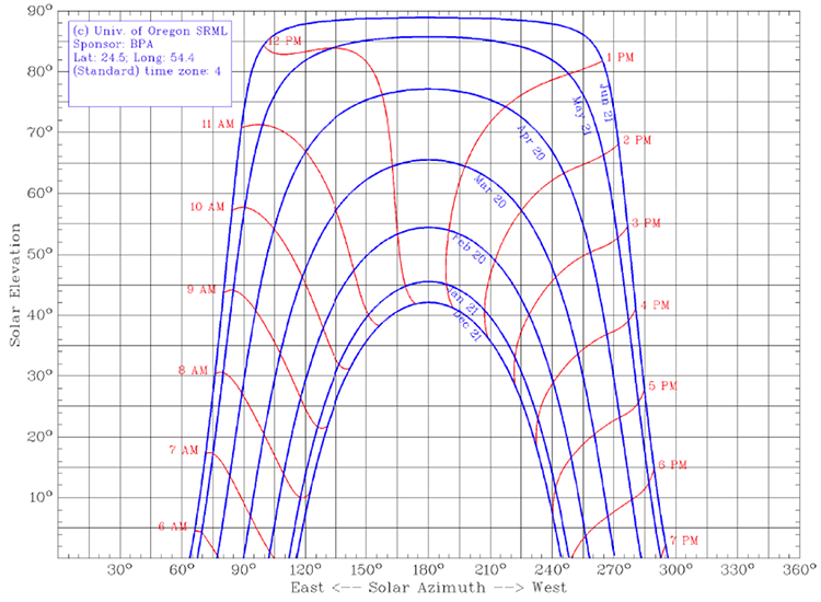
In this diagram, the solar altitude (elevation) is plotted versus solar azimuth, as shown by the blue curves for each date. There are a few representative dates shown, and January 21 is the closest to the calculation example previously given. Note that the solar azimuth is given on the 360o scale, with 180o corresponding to the south. Alternatively, Kalogirou uses the coordinate system and formulae to calculate solar parameters versus 0o as true south, with negative azimuth values corresponding to morning and positive azimuth values corresponding to afternoon hours. So beware of that difference if you try to match data from both sources. On the Sun Path diagram, the hourly position of the sun is marked by the red curves. In this particular case, the local standard times are plotted, while a similar diagram can be made in terms of solar time.
Check Your Understanding - Questions 1-3
Check Your Understanding - Question 4
Is it possible for the sun to reach 90° altitude at any time in a year in the following states? Type "yes" or "no" for each location. Can you explain why?
Arizona
Pennsylvania
California
Hawaii
Problem 3-1: Solar path calculation
(This calculation will be submitted as part of Lesson 3 problem set).
- Go to the Sun Path Chart Program calculator [33] and calculate the sun path for a location of your choice. Use the orthogonal projection. Save your diagram.
You may need to find geographical coordinates and time zone for your location as input. Here is one of the websites that can be conveniently used for that purpose: TimeandDate.com [34]. Just type in your location and get the data.
- Using equations (3.1) and (3.2) in this lesson, perform a manual calculation of the sun position (solar altitude and solar azimuth) for the same location on February 20th, at 12 pm and 3 pm local time.
- Mark your manual points on the diagram. Are you able to match your calculations with the plot?
The above materials and activity make sure that you can employ proper tools for defining solar position on the sky dome. Further on, the receiver positioning algorithms will use this information as the operational basis. Different types of tracking systems are discussed in the next section of the lesson.
Additional Reading
NREL Report: Reda, I.; Andreas, A. (2003). Solar Position Algorithm for Solar Radiation Applications. 55 pp.; NREL Report No. TP-560-34302, Revised January 2008. [35] (1.9 MB PDF Document)
3.3. Cosine Effect
3.3. Cosine Effect
In technical sense, sun tracking is a method to keep the surface of the solar panel or a collector perpendicular to the incident solar rays. This is the ideal condition, when maximum amount of solar energy is transmitted to the receiving surface.
When the incident ray is not perpendicular to the surface (which is often the case with fixed-tilt systems), the angle of incidence is not zero (q ¹ 0), and part of the incident energy will be lost due to so-called cosine effect. To maximize efficiency of the system, we should always seek ways to minimize the cosine effect at any particular moment of time.
The figure below shows two scenarios: the left image illustrates an ideal situation, when solar rays come down on the surface of solar collector (PV panel) at the 90o angle; the right image shows what happens when the Sun moves across the sky while the panel remains fixed.
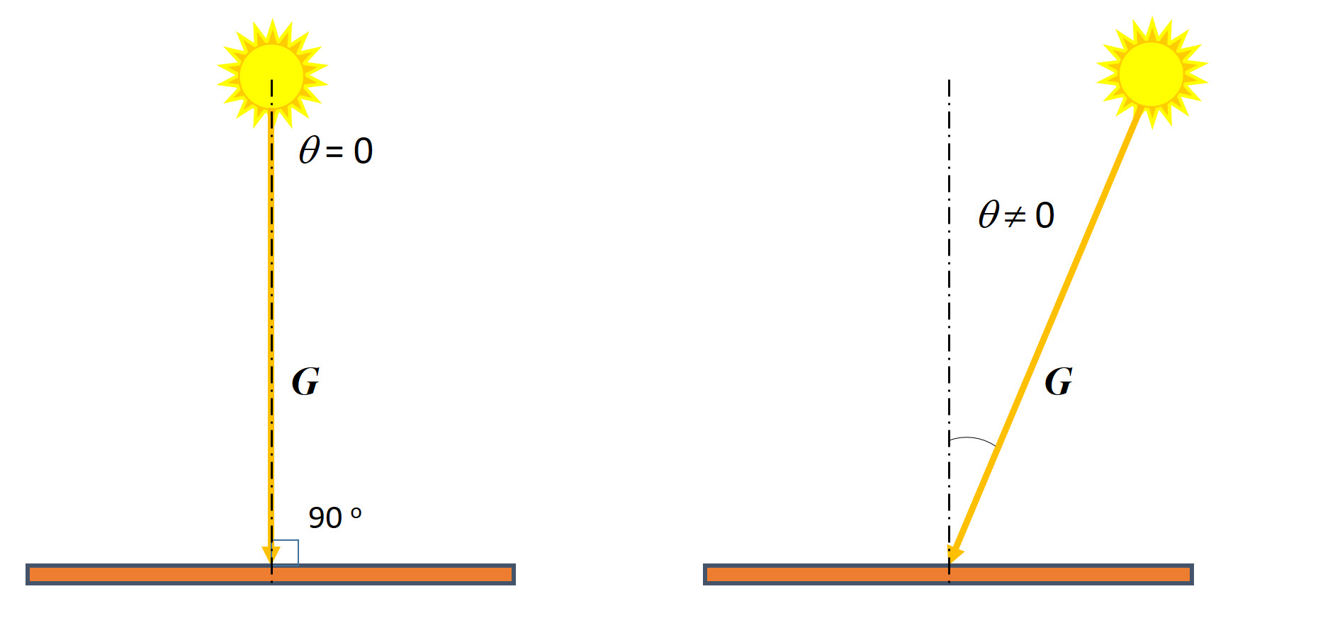
In the second case, the sun rays come down to the surface at an angle q, which will decrease the amount of energy absorbed by the surface, and thus will lower the system efficiency. By how much?
We can try to estimate this reduction due to cosine effect if we break down the G vector into two components: one perpendicular to the surface (G^) – useful component that would be absorbed, and one - parallel to the surface (G||) – non-useful component that would be reflected or somehow lost.
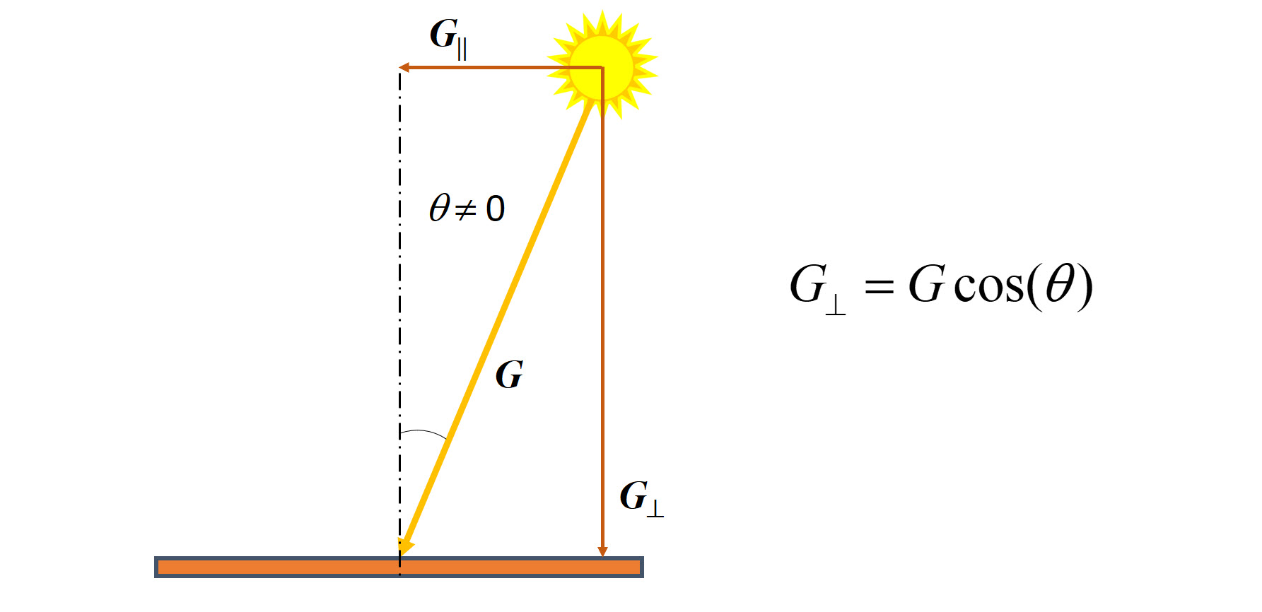
For example, if we assume incident irradiance to be 1000 W/m2, and angle of incidence 30o, then
G^ = 1000 x cos(30o) = 866 W/m2
Thus, without considering other inefficiencies, losses due to cosine effect are expected to be around 13.4% at this angle, which is quite substantial.
Tracking can be an effective solution to minimize these performance losses. Tilting the panel by the angle (b) equal to the zenith angle would set the panel perpendicular to the sun rays once again.
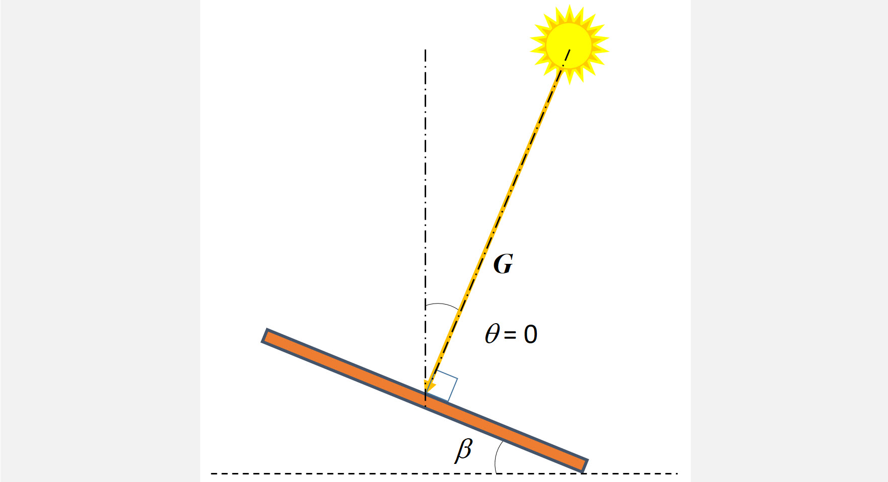
The early attempts to eliminate cosine effect would involve annual adjustment of panel angle throughout the day. But that would be tedious, inaccurate, and too discrete, while the Sun stays in constant motion on its daily path. Present-day automatic trackers use algorithms that are able to continuously track the Sun with accuracy of ±0.0003o.
3.4. Types of tracking systems
3.4. Types of tracking systems
Tracking systems are classified by the mode of their motion. We can define three axes for a moving surface (which represents a receiver): two horizontal axes and one vertical axis (Figure 3.3). The surface can be rotated around each axis (tilted) to achieve an appropriate angle with respect to the incident solar beam. When movement or adjustment of the surface is done by rotating around one axis (tilting), it is single-axis tracking. When rotation of the surface is done around two axes simultaneously, it is two-axis tracking. Two-axis tracking allows for the most precise orientation of the solar device, is reported to provide 40% gain in energy absorption, but it is more complex and costly. Such two-axis systems are also used for controlling astronomical telescopes.
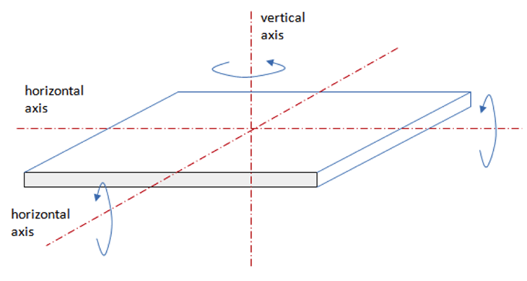
In case of single-axis tracking, the axis of rotation is usually oriented in the N-S direction or E-W direction. Tilting is performed in a way to minimize the incidence angle. In case of two-axis tracking, ideally, the incidence angle is always zero, i.e., the surface is kept perpendicular to the solar beam.
Read about various tracking modes in the following sources.
Reading Assignment
Book chapter: Kalogirou, A, Solar Energy Engineering, Chapter 2: Environmental Characteristics. pp. 64-71. (See E-Reserves via the Library Resources tab.)
This reading is the continuation of the same chapter you read in the previous section of the lesson. It describes different types of single-axis and dual-axis tracking systems and compares their performance by the amount of received solar energy.
Book chapter: Brownson, J.R.S., Solar Energy Conversion Systems, Chapter 7. Applying the Angles to Shadows and Tracking, pp. 192-196. (See E-Reserves via the Library Resources tab.)
This reading gives a few more descriptions of tracking modes, some different from those listed in Kalogirou's book. You will also read here about specific advantages of particular types of tracking systems.
So, from reading these chapters, you now have quite complete list of different ways of tracking, and corresponding formulae to describe the relative position of the sun and inclined surface. The following activities will give you an opportunity to practice the basic calculations involved in two-axis and single-axis tracking. The first problem considers a simple case of two-axis tracking. As long as we know the solar coordinates, we can orient the receiver in that direction. But the tracking system that moves the plane needs precise input data, which we try to obtain here.
Problem 3-2: Dual-axis tracker data
The system is a heliostat with two-axis tracking: one vertical axis, and one horizontal (SN) axis. The goal is to determine the azimuth for the heliostat orientation and tilt angle for the horizontal axis at any time of the day to supply these data to the tracking system. A sketch of the collector is given below, and the blue line is the horizontal axis we want to tilt. The red line denotes the vertical axis, about which the collector can be rotated.
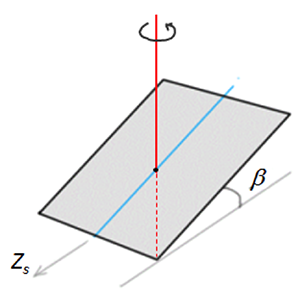
Calculate and tabulate a set of Zs-β data for every hour during the daylight period on March 21 at your chosen location. Feel free to use any available resources (solar path diagrams or appropriate equations) to determine the position of the sun.
In this calculation, we can assume that incidence angle on the surface of the collector will be zero at any moment.
Please provide references and explanation to your work.
This calculation will be submitted as part of Lesson 3 problem set.
The second problem on this topic considers the single-axis tracking case - one with horizontal NS axis and EW tracking (see Kalogirou's chapter, p. 69). In this case, the receiver has only one degree of freedom, so its motion is limited. We will not be able to reach the zero incidence angle, but we will try to minimize it in order to maximize the solar radiation on the plane.
Problem 3-3: Single-axis tracker data
Consider a flat collector with a fixed horizontal NS axis and tilting EW axis (see sketch below, side view). Because the NS axis is fixed, the surface azimuth (Zs) is either -90o when it tilted east, or +90o when it is tilted west. The β angle defines the tilt, which is applied to minimize the incidence angle on the surface.
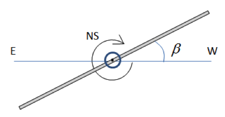
For your chosen location, determine and tabulate the surface position parameters (Zs-β ) for every hour on March 21st. Feel free to use any available resource to determine the sun position. Make sure to provide references and explanation to your work.
This calculation will be submitted as part of Lesson 3 problem set.
3.5. Engineered devices for solar tracking
3.5. Engineered devices for solar tracking
The main elements of a tracking system include [Rockwell Automation, 2011]:
- Sun tracking algorithm: This algorithm calculates the solar azimuth and zenith angles of the sun. These angles are then used to position the solar panel or reflector to point toward the sun. Some algorithms are purely mathematical based on astronomical references, while others utilize real-time light-intensity readings.
- Control unit: The control unit executes the sun tracking algorithm and coordinates the movement of the positioning system.
- Positioning system: The positioning system moves the panel or reflector to face the sun at the optimum angles. Some positioning systems are electrical and some are hydraulic. Electrical systems utilize encoders and variable frequency drives or linear actuators to monitor the current position of the panel and move to desired positions.
- Drive mechanism/transmission: The drive mechanisms include linear actuators, linear drives, hydraulic cylinders, swivel drives, worm gears, planetary gears, and threaded spindles.
- Sensing devices: For trackers that use light intensity in the tracking algorithm, pyranometers are needed to read the light intensity. Ambient condition monitoring for pressure, temperature, and humidity may also be needed to optimize efficiency and power output.
- Limit switches are used to control speed and prevent over travels. The mechanical over travel limits are used to prevent tracker damage.
- Elevation feedback is accomplished by either 1) a combination of limit switches and motor encoder counts, or 2) an inclinometer (a sensor that provides the tilt angle).
- An anemometer is used to measure wind speed. If the wind conditions are too strong, the panels are usually driven to a safe horizontal position and remain in the safety position until the wind speed falls below the set point.
Three classes of tracker drive types to operate the moving receiver:
- Passive trackers use the sun's heat to expand the compressed gas, which is used to move the panel. Selective heating of some cylinders versus others create more expansion on one side of the panel and make it tilt. These systems are relatively simple and low-cost, although may lack due precision necessary for the solar conversion systems using concentrated sunlight.
- Active trackers use hydraulic or electric and an actuator to move the panel based on sensor response. Light sensors are positioned on the tracker at different locations for higher precision. These systems work best with the direct sunlight and are less efficient with cloudy skies.
- Open-loop trackers use pre-recorded data on the sun position for a particular site. Simple timed trackers move the panel at discrete intervals to follow the sun position, but do not take into account the seasonal variations of the sun's altitude. The altitude/azimuth trackers employ astronomical data to determine the position of the sun for any given time and location.
Actuators
Linear actuators are common technical tools that proved to be effective solution for moving the solar receivers. An electric linear actuator is a device that converts the rotational motion of an electric motor into linear motion. With linear actuators you can lift, slide, adjust, tilt, push or pull objects of various mass, and they are easy to implement in many different applications. Mechanically, linear actuators are quite simple devices that have been extensively deployed in 2-axis and 1-axis trackers due to their precision and service reliabilty.
The following video provides a rather detailed overview of the design, principle of operation, and specifications of electric linear actuators:
Video: Linear Actuators 101 (19:43)
Hello, everyone. In this video, I'm going to be talking about linear actuators. Linear actuators are really cool. And in this video, I want to explain what they are, how to use them, how to drive them, and how to pick them based on the various specs for your application. So, let's get started.
So, first off, what is a linear actuator? Well, really, linear actuators are just motors, but instead of moving around in a rotational direction, they move in and out along a linear plane. So, a normal motor would spin around like this. It just kind of spins, and it spins indefinitely. If you apply voltage one way, it goes this way.
If you apply it the other way, it goes the other way. Whereas linear actuators, when you apply voltage to the motor, the shaft here either goes out this way, or if you reverse it, it goes back the other way. Ultimately, you drive them in the same way that you would a standard DC motor. If you go positive to positive, negative to negative, it will go usually out. And if you flip the polarity of those around, it will go the other way.
I will be taking one of these apart later so that you can kind of see how it works. But as you can see, each one of these basically has this big motor on the end of it. Right there, right there and right there. And that motor spins around, essentially a lead screw, which pushes that lead screw out or pushes it back in. Now, with standard rotational motion, there are no end stops.
It kind of just keeps spinning indefinitely. But when you have something like this, there is an end stop to where it can hit the end on the extended travel, or it can come all the way back in. And there's a couple of little mechanisms that stop that from basically causing damage to the actuator. But that's really all there is to it. You can use these in any application where you want linear motion rather than rotational motion, like lifting up forks on something.
They're used a lot of times in combat robots for lifting up, clamping down. Or I used it in my little wheelchair snowblower thing for actually lifting the blade up and down. They are really good for any kind of linear motion. Just like with standard DC motors, there's a lot of various sizes and configuration to linear actuators, but ultimately, they all pretty much do the same thing. They provide linear movement.
There are a couple different variations that you need to look out for when purchasing a linear actuator for your application. If we look at the end of this service city one, we see that there are five wires coming off the end of it. And if we look at these two that I salvaged from the wheelchairs, there are two wires and two wires. Now, the difference is all of these can be driven just like a standard motor. You apply voltage, it goes out, you switch the voltage, it goes back in.
However, this one actually has a feedback mechanism inside of it. What I was saying earlier about the shaft reaching the end of travel, on either extreme, all of these have some sort of protection mechanism or some sort of electronics inside that stop them from overextending themselves. It's usually in the form of just a diode, so that when it goes out to the far end of its reach, the diode will stop current from flowing in that direction, and then you can only reverse it back the other way. Almost every linear actuator has that. There's probably some exceptions.
I'm sure there's some really cheap ones out there that don't have that, but generally speaking, that's a feature of a linear actuator. So, what does the servo city one have that is different? And this isn't unique to servo city, by the way. It's just the one that I have here that has the feedback mechanism inside of the base of this. When I open up, you'll see it in better detail.
There is essentially just a potentiometer that is connected to this output shaft, and it is, I guess, wired proportionately so that when this shaft is all the way in, that potentiometer is at one end of its range. And then when this shaft is all the way out, it is at the other end of the range. And this happens to be a ten k potentiometer. So here it's going to read zero, and all the way out there it's going to read ten kilo ohms. So this is very useful when hooking up to a motor controller or something else to determine pretty much where this is in the travel.
Now, with both of these, they were for a wheelchair, I think this was like the power lift for the seat, and this was like a tilt for the seat, something like that. You're less concerned with where that is. And in some applications, you might not really care where this shaft is. You just kind of want to move it forward and backward, much like a standard motor. You just want to move it at a certain speed in a certain direction.
So that is something to look out for, is some of them do have some kind of feedback mechanism, and others do not. You might not need it, or you might need it. The other thing to look out for is some of these are actually linear servos. So, they take it one step further, and they actually take the motor controller and put it directly inside. So, you control it much the same way you would with a servo.
You just send it a pulse command, and then it travels wherever you dictate. So if you say, I'm going to give it this pulse, then it would go halfway, or you can go like 80%, 20%, whatever it is. And so linear servos are very different. Servo city does have a very good video that shows you the difference between a standard linear actuator, one with feedback, and a linear servo. So that's worth checking out.
And that is linked below. But that is something that you might want to look at, because not all of these have the exact same features inside of them. Driving linear actuators is pretty straightforward because they are just motors. So, you drive them the same way you would a standard motor. I have these leads connected up to my benchtop power supply over there, and this has 12 volts on it.
So if I connect one lead down here and then the other one up there, this will just start moving. There we go. So, it's moving in. And if I switch these around, this one up here, it will move out once I clip it in. Right?
And now it moves out the other way. As you can see, linear actuators are not the fastest thing in the world. There's a lot of power. There is absolutely no way I could stop this from moving, but they are relatively slow, and I will get into that a little bit later. But the speed at which these move is one of the things that you should factor in when you are picking these out.
So if we look over at the Servo city, we have all these five wires coming out. We can just ignore these three for now, and then we can connect it and control it the exact same way. I'm just going to go red to red and black to black. This one is a little bit zippier, and then we can reverse it and it will go the opposite direction. So, it's really that simple.
And some of these actually do come with a little toggle switch that is pre wired for these. But if you don't have that, or if you want to make your own, you can use any dual pole, dual throw switch. Basically one that has six connections like this. You wire a power supply into the middle. One side is one polarity, and then the other side is a different polarity.
So let's say this is red from the supply, this is black from the supply. You would just go red and black directly to the motor, but in this side, you would actually flip them to the other side. And I will have a link to a wiring description down below if that's confusing. But you're going to want a motor that is not latching like this one. You're going to want kind of a toggle that goes like a normal toggle switch.
This isn't the right one to use, and I didn't have one on me, so I won't show that. In addition to using just a simple switch, which will just go full speed one direction or full speed the other direction, you can use a motor controller. The main difference between using just a switch directly up to a power supply and a motor controller is with a motor controller like this, Roboclaw is, you can actually vary not only the speed, but the direction on the fly. This you can connect to a microcontroller. You can connect it to all sorts of other things.
And this is what I'll be using for my application. But the real big difference is controlling the speed and other parameters. This can actually also accept the encoder feedback, and we can do all sorts of fun things. But for basic control, you really don't need anything, really, beyond a switch and a power supply. So they're pretty easy to drive.
Now it's time to disassemble this, dissect it, and show you what's going on inside the linear actuator. I'm using the servo city one only because it's actually the most well laid out and the easiest to get into. So let's just start taking it apart. There's three screws at the bottom of this, so I'm just going to go ahead and take those out.
You can see we've got some plastic gears around here, and at the very bottom, you can see that is our potentiometer. Now, don't fear, these plastic gears actually have nothing to do with the driving of the actuator. This is just for the feedback side. So I'm going to take this off, take this shell off, and then we can actually see the gears that are driven by the motor directly. But this is, I want to say, maybe probably a five turn or ten turn potentiometer.
And it spins directly with the output shaft, and that gives you the feedback that ends up going on these main wires. So, it's a pretty simple little mechanism that as this main output shaft turns, it also turns the potentiometer. And then you just read the potentiometer. So, nice and simple. All it.
So, now that we've got this open, there's yet another gasket here. And then you can see all the output gears. Let me see if I can get a little bit better shot of that. So you've got the motor right there, and that is a plastic pinion gear. And then it moves into all the metal gears right here.
So this particular motor comes in a couple of different configurations. And ultimately, the difference between the stroke or how far this travels out is really just going to be the gear reduction here, because the pitch of the linear rail inside here, all of that good stuff. But this is just the gear train that slows down the motor and drives the linear actuator inside this shell. And you can see you've got a lot of decent gears in here. There's a lot of nice oil.
So awesome. That is pretty cool. So that's really all there is to it inside, it's just basically a really simple gearbox that drives a linear shaft over here. So, let's take this outer shell off, and then you can see what's inside of here. It.
So there you go. There's a little gasket that goes all the way at the bottom down here. Let's get that out of the way. And then you can see we've got two little micro switches. One here and then one here.
And then we have a couple of diodes in place. Now, this one does not appear to have adjustable end of travel. So, basically, as this comes down, it will hit against there. And as it goes out to this side, it will hit against there. So, it's just this little nub or this little piece right there that travels up and down and is hitting your end stop.
So, pretty cool. Some of the higher end ones actually do have adjustments. So, where you can kind of slide these along and you can have different end stops. However, this one does not have that. So you would need to rely on software to do that.
And if you do use something like the roboclaw, which I misplaced, if you use something like this roboclaw, you can actually put that into the software in here and configure that separately. And then right here, you can see we just have a simple lead screw right there, and it's all nice and greased up. And then this just simply slides along the lead screw. So when the motor turns, it turns these gears, it turns this and that, either presses this out or brings it back in. It is really that simple.
There's not a whole lot to it. And then this is just a cover to protect the whole thing. So, yeah, that's all there is to a linear actuator. Let's put this back together. Okay, so we've talked a little bit about what a linear actuator is, how it functions.
Taken a look inside and I've kind of covered the very basics on how to control them, either directly with a power supply or just wiring them up to a switch. If you want to take this further, I will be doing another video as a supplement to this that shows you some of the more, I guess, advanced parts of controlling these with something like the roboclaw or another type of motor controller. That's a little bit beyond the scope of this video, but I will be coming out with that separately because I am working on my own project using a couple of these linear actuators. So, the next thing that we need to talk about is how to spec them for your project. As I discussed earlier, linear actuators are essentially just motors, and you can treat them the same way in terms of specking them out.
For your project, you're going to need to pay attention to the voltage that the motor runs at and the current requirements behind that. And really you can run these at different voltages and that's a larger discussion. But essentially the amount of voltage that you put into a DC motor is going to proportionately relate to how fast it spins. However, if you over voltage, a DC motor apply more voltage than it is speced at, you will lessen the lifespan of that motor. So keep that in mind.
And a lot of these have a duty cycle rating that is only like 25%. I. E. This is not meant to run 100% of the time. It is spec to run 25% of the time.
Now, the big difference in driving these motors with just a power supply directly and driving them with a motor controller like, let's say the roboclaw is going to be being able to vary the speed. If you put 12 volts into this motor, it's always going to run at that exact same speed, either forward or backwards. It's always going to be the same. If you use a motor controller, that gives you the opportunity to control it at different speeds. And that's really the only reason why you would want to use a motor controller, is to vary that speed of how fast the shaft moves.
There are a couple specifications for linear actuators that are unique to them, and you won't find them on a normal DC motor like the voltage and the current. You're going to want to pay attention to the stroke. The stroke is probably the most important part of the linear actuator. And it basically means how far the shaft can travel. It's a total travel, not necessarily the total size of it, but just how much it can travel.
This one is a twelve inch, meaning when this is all the way in to all the way extended, it moves twelve inches. These are somewhere around like six inches. So definitely pay attention to the stroke. The other spec that you're going to want to pay attention to with a linear actuator is going to be the load rating. There's going to be two load ratings.
Usually there's going to be the dynamic load and the static load. The static load is quite simply how much force can you put against this before it will fail statically? So let's say it was just sitting there like that and it had a load on top of this. This one's rate, I think like a 500 pound static load. It means it can just sit there with 500 pounds resting on it without failing.
The dynamic load is how much force it can actually exert on the thing that you're trying to use it with. I want to say this one's rated like 100 and 5175 pounds. So that means it can actually press or exert a force of 175 pounds. So that is the difference between a static and a dynamic load. The last thing that you want to look at is the speed at which these things move.
Usually it's some kind of like inches per minute or something like that, and it's going to be how fast it can move. That's something that you really want to pay attention to because this has a twelve inch stroke. Let's say it was one inch per hour. That means it's going to take 12 hours to fully extend from fully non extended. So that is something you really want to pay attention to.
Now, when you look at these linear actuators, you will see that there's usually multiple variations of the same thing. For Instance, with this model, there are, I think, three different versions of it, and they're all the exact same price. One of them has like a 50-pound loan rating. One's like 100 and 5175, and the other is like 500. Let's say.
Why are they all the same price? Why wouldn't I go with the one that's like rated 500 pounds? Well, there's no free lunch here. These all have a fixed amount of power that they contain, and power is equal to work done over time. So guess what?
That one that has the really high load rating is also going to be incredibly slow because it is the amount of work done over time. You're doing it in a lot longer time, so then the work can be a lot higher. And likewise, on the other side of the spectrum, a really fast one just can't do as much work because it's doing it in a much shorter period of time. So that's something you want to pay attention to when you're specking. These is not only the stroke, which is how much they can move, but how fast they can move.
And then of course, you want to pay attention to the static load rating because if you're trying to lift something really heavy, but something's pushing against it, you want to make sure that it can handle those static forces as well as the dynamic ones. So I think that's about all I wanted to talk about with linear actuators. I think the last point to talk about is where to find them. These two were salvaged from an electric wheelchair. I do a lot of electric wheelchair salvaging because there's a lot of good parts in there.
Look for some that have a dead battery, dead charger, dead controller, and you can usually find a linear actuator in there. If they have some kind of tilting seat mechanism, usually the fancier ones do. Just keep in mind the voltage is almost always going to be 24 volts and they are going to be a weird form factor that might be really difficult to use. And typically, they have a very short stroke and they are very, very slow. So there's a lot of caveats to getting them free out of a wheelchair or really inexpensive out of a wheelchair.
But you can find them on eBay. There's a lot of sellers that have them on eBay, and there's a lot on Amazon. Just keep in mind, the ones on Amazon and eBay tend to not have any feedback. They're just two wires. Some of them do have feedback, but they tend to start getting kind of pricey.
And sometimes the load ratings are not really exactly what you're looking for and they have limited strokes, stuff like that. Also, you might want to check out Servo City. Servo City has a really nice selection of them, and I'm not just simply plugging them. They really do have a nice selection of linear actuators in all shapes and sizes. So it's at least worth a look to see what's available for your project.
As always, thanks for watching this very long and informative video on linear actuators. You can check out my Facebook page for all my little project updates and such. And down below there's a lot of links that you can check out. There's an Amazon link down below that. If you use and shop with Amazon using that link, you can give a little bit of a kickback to my channel to help support my projects and my videos.
As always, thanks for watching. See you next time.
The technical details of all the components of tracking systems would be beyond the scope of this course. It is important to understand though that additional components and more complexity, while improving efficiency of the solar panels and reflectors, add to the cost of the whole system and consume additional energy.
This following video (4:25) demonstrates some technical features of a single-axis tracking system:
Video: Renewable Energy: Single-Axis Tracker (4:24)
THOMAS JENKINS: Here we have an example of something that might be at more of a commercial application of photovoltaic systems. We have several photovoltaic panels. We have two sets, we have one type on this structure, we have another type on the structure behind it. Both are mounted on what's called one-axis trackers, in that there are electric motors which turn these panels such that they track the sun as it goes from the east to the west.
With this type of tracker, it's fairly sophisticated in that it's a computer-controlled tracker. There is a little computer in here that runs some very sort of mid-complexity algorithm that knows the latitude of your location, where you are-- Las Cruces, New Mexico, 32 degrees latitude-- and it knows the day of the year-- for example, January 28, day 28-- and it knows the time of the day-- 2:00.
With that information, it can predict exactly the angle of the sun, relative to east and west, and it knows to turn the tracker exactly that many degrees every day to point directly to the sun. This increases the efficiency or the amount of electricity that comes from the solar panels, but you have some additional complexity in your system. These are what's called active trackers, in that it requires electrical motors, it requires some mechanical components, some electrical components, and it tracks the sun, but you get more electricity from this type of system.
This system is a German design, and it's being tested here at SWTDI. Right next to it, we have a good bit of data collection that is brand new, very sophisticated, and it's connected via cell phone and land lines such that all the data-- which is being collected real time-- can be accessed through a cell phone from anywhere in the world. For example, at the headquarters of the German company, who's looking at the system design and the system components and seeing how they're interacting.
You can see on this structure here that we have a couple of instruments that are being used to characterize the sun's energy. These are called pyranometers. They are reading the amount of sunlight so we know how much energy is striking the surface. And, from that, we can see how much energy the panels are delivering to us and determine the efficiency of the panels. So a lot of instrumentation is going in this because this is an evaluation system, but this might be a system that might go into, for example, a desert environment over several acres that might be a large scale electrical production.
Tracking the sun, in some cases, is very important, especially on systems that use a new type of system with lenses, called Fresnel lenses that are used to concentrate the sun onto a smaller section of photovoltaic, so the total amount of photovoltaics that you need is smaller, but they produce the same amount of energy because you're concentrating the sunlight onto the cell. So we're looking at two different types of modules on the same structures, under the same ambient conditions, the same location, the same amount of sunlight, and we're comparing those, seeing how efficient they are relative to one another and relative to traditional solar photovoltaic systems.
PRESENTER: The preceding was a production of New Mexico State University. The views and opinions in this program are those of the author and do not necessarily represent the views and opinions of the NMSU Board of Regents.
Additional Reading
Journal paper: Mousazadeh, H. et al., A review of principle and sun-tracking methods for maximizing solar systems output, [39] Renewable and Sustainable Energy Reviews 13 (2009) 1800–1818.
Summary and Activities
Summary and Activities
In Lesson 3, we discussed the benefits of sun tracking for performance of the solar energy conversion systems. It is clear that although tracking helps to collect more solar radiation per square unit of solar receiver, the tracking systems may be complex and costly, and hence should be used only when benefits in terms of efficiency outweigh the expenses for extra energy and equipment. We reviewed the fundamentals of solar motion, and you should now be comfortable using the key equations to calculate the sun position at any time at any location on the earth. This lesson included description of different modes of tracking - single-axis and two axis - and gave you an opportunity to perform some basic calculations and work with available data on solar path. I hope you found the resources in this lesson useful and that, in the future, you will feel confident applying those calculation methods to the systems of your choice. Tracking certainly is a worthy technology when we look at the utility scale solar systems, as this technology provides an even more significant boost when scaled up. A number of companies are currently specialized in tracking technologies, constantly innovating and creating more and more robust systems for future solar plants.
The table below summarizes all activities that are due for this lesson. Some of those have been included in the body of the lesson, and this list simply repeats them for your reference.
| Type | Description/Instructions |
|---|---|
| Reading | Complete all assigned reading for this lesson. |
| Discussion | Discussion "Tracking systems": Lesson 3
|
| Written Assignment | Problem set on sun position and tracking Please complete the Problem Set posted within this lesson (you can also download this problem set as a single document from Canvas module):
You can type your solutions or hand-write them and scan to a PDF file (just make sure that all is legible). Submit your work to the respective Dropbox in Lesson 3 Module. |
References for Lesson 3
Barbose, G., Darghouth, N., Weaver, S., and Wiser, R., Tracking the Sun VI. An Historical Summary of the Installed Price of Photovoltaics in the United States from 1998 to 2012. US Department of Energy, July 2013.
Brownson, J.R.S., Solar Energy Conversion Systems, Elsevier, 2014.
Kaligirou, A, Solar Energy Engineering, Elsevier, 2014.
LINAK Group Inc., We Catch the Sun [40]. 2015.
Rockwell Automation, Solar Tracking Application [41], White Paper. 2011.
UO SRML - University of Oregon, Sun Radiation Monitoring Laboratory, Sun Path Chart Program, 2007.
Wikipedia [28]
Lesson 4: Photovoltaics
Overview
Overview
This lesson contains materials describing the main principles of photovoltaic conversion of light. You will learn what properties of PV materials determine the performance of the solar cells, and how that performance is measured. You should be able to look at the performance curve and say if it is good or not, if you deal with a single cell or a module. We will also see what happens to the parameters of the PV actions on system scale-up. Different types of PV materials and systems will be discussed here, and recent innovations and trends to improve solar cell efficiency will be reviewed.
Learning Outcomes
By the end of this lesson, you should be able to:
- understand and explain the principle of photovoltaic effect;
- analyze the photovoltaic cell performance data;
- discuss innovative ideas and recent trend in PV development.
Readings
Duffie, J.A. and Beckman, W.A., Solar Engineering of Thermal Processes, 4th Ed., John Wiley and Sons, 2013. Parts of Chapters 2 and 7. Please refer to particular sections of the lesson for more specific assignment.
Honsberg, C and Bowden, S., Photovoltaic Education Network [42], Accessed: May 2020.
Kalogirou, S.A., Solar Energy Engineering. Processes and Systems. Elsevier, 2009, Chapter 9. Photovoltaic Systems, pp. 483-486.
4.1 Photovoltaic effect
4.1 Photovoltaic effect
The word "photovoltaic" immediately indicates the connection between light (phot- greek) and electricity (volt, unit for electric potential). The key property of a photovoltaic material is to convert light energy to electric current. This conversion takes place due to the photovoltaic effect - a physical phenomenon in a semiconductor, which we are going to discuss next.
Semiconductors are a special class of materials, whose conductance is not permanent, but rather depends on the energy available to activate electrons in the crystal lattice. Crystalline silicon is a semiconductor material widely used in photovoltaics. It becomes conductive when the energy of the photons absorbed by the crystal surface is sufficient to raise the electron state from the valence band to the conduction band. This required amount of energy to excite an electron is defined as band gap. Band gap is an intrinsic property of semiconductors and eventually has a direct influence on the photovoltaic cell voltage. The following schematic (Figure 4.1) provides a demonstration of the band gap concept.

In this picture, we can visualize the difference between different classes of materials: conductors (metals), semiconductors, and insulators. The valence and conduction bands in a metal overlap, so it does not take any significant energy to free the electrons. They are available for conduction as soon as the potential gradient is provided. In insulators, the gap between the valence and conduction bands is very large, so it requires so much energy to free the electrons that it can damage the material itself. For semiconductors, the situation is somewhere in between. The band gap is big enough to prevent spontaneous conduction and to provide separation of charges, and small enough to be matched by photon energy.
The band gap energies of several different materials are listed in Table 4.1 below. Some of those materials are more suitable for photovoltaic applications than others. How suitable the materials are for photovoltaic applications would be determined by how close the photon energy is to the band gap of the material, and if the energy of photon is sufficient to cover the band gap.
| Material | Band Gap (eV) | |
|---|---|---|
| Si | Silicon | 1.11 |
| Ge | Germanium | 0.67 |
| CdTe | Cadmium telluride | 1.5 |
| Cu2O | Copper oxide | 2.1 |
| Cu3N | Copper nitride | 1.75 |
| GaP | Gallium phosphide | 2.26 |
| GaAs | Gallium arsenide | 1.43 |
| PbS | Lead sulfide | 0.37 |
| Si3N4 | Silicon nitride | 5 |
| C | Diamond | 5.5 |
| SiO2 | Silica | 9 |
For example, if we have a photon with energy of 2 eV hitting silicon surface, 1.1 eV of that energy will be used to move an electron to the conduction band; the rest of the energy (0.9 eV) will be dissipated as heat. However, if a material with a greater band gap is used, for instance copper oxide, 2 eV is not enough to free the electron. We would need a higher energy photon there.
By the way, you may remember from physics that photon energy is dependent on the wavelength of light. The shorter the wavelength (λ), the higher the frequency of the light (ν), and the more energy it brings:
(where h is the Plank constant, and C is the speed of light)
For instance, for the red side of the visible light spectrum, , so we can find:
At the same time, for the violet side of the visible spectrum, , and:
Obviously, the photons associated with high frequency radiation (violet, UV) deliver more energy and can be used with larger band gap materials.
Check this out
Photon energy calculator from the PVEducation website. [45]
Check the numbers given in the above example. You may also want to see what light wavelengths would be suitable for the materials listed in Table 4.1.
Based on these reflections, we see that low band gap materials (such as germanium), can be used to capture low energy photons (like those in the red and IR parts of the spectrum), and high band gap materials (e.g. copper nitride or gallium phosphide) can be used for using high energy photons. Combination of different materials in one system allows for more efficient use of available radiation. At the same time, if the band gap of the PV material is too small compared to the incident photon energy, a significant amount of energy will be converted to heat, which is not a good thing for PV cell itself. No matter how much higher the photon energy is compared to the band gap, only one electron can be freed by one photon. This is the reason for the limited efficiency of the photovoltaic cells.
The data in Figure 4.2 show how the maximum efficiency of a solar cell depends on the band gap. If the band gap is too high, most photons will not cause photovoltaic effect; if it is too low, most photons will have more energy than necessary to excite electrons across the band gap, and the rest of energy will be wasted. The semiconductors commonly used in commercial solar cells have band gaps near the peak of this curve, for example silicon (1.1eV) or CdTe (1.5eV). The Shockley–Queisser limit (33.7%) defined at the peak of the curve has been exceeded experimentally by combining materials with different band gap energies into tandem solar cells.

Next, please refer to the following reading to learn more about the background of the photovoltaic effect:
Reading Assignment
Brownson, J.R.S., Solar Energy Conversion Systems, Chapter 14: Systems Logic of Devices: Optoelectronics, pp. 349-356. (See E-Reserves via the Library Resources tab.)
Based on the above reading, we can summarize that the photovoltaic effect essentially includes three main steps:
- Absorption of light (photons)
- Generation of charge carriers
- Separation of charge carriers between electrical contacts
When all these steps occur, the system is able to generate electric current (flow of charge carriers), which can do work.
Answer the following questions for self-check:
Check Your Understanding - Question 1 (Multiple Choice)
Check Your Understanding - Question 2 (Essay)
Calculate the photon energy corresponding to the radiation wave length of 500 nm.
Check Your Understanding - Question 3 (Essay)
List three main stages of the photovoltaic effect:
4.2 P-N Junction
4.2 P-N Junction
While photovoltaic effect readily takes place in a number of materials, the third step - separation of the charge carriers - is probably most tricky from the technical point of view. For example, in a regular silicon crystal, when absorption of a photon induces the release of an electron from the valence to the conduction band, a hole (positively charge locus) is formed in its place in the crystal lattice. Further, the excited electron and the hole can recombine to release heat. This is not what we want! So doping is often used to modify silicon structure. For example, boron (B) can be included into the structure in place of silicon. Because boron has valence of 3 (versus silicon valence of 4), there is a "gap" in the structure, which can accept an electron. This type of semiconductor, which has positive centers to accept electrons, is p-type semiconductor. Alternatively, silicon can be doped with phosphorus (P), which has valence of 5 and brings an extra valence electron, which is not involved in covalent bonds. This electron can be donated. This type of semiconductor is n-type semiconductor.
Thus, the p-semiconductors have excess of positive charge carriers, and the n-semiconductors have excess of negative charge carriers. If p- and n-types are put together, the interface between them will represent the p-n junction.
To understand how the p-n junction works, please watch the following video (10:36):
Video: The PN Junction. How Diodes Work? (10:36)
We can find semi-conductor PN junctions in many places. They form part of electronic and opto-electronic devices, such as solar cells, that transform solar energy into electrical energy, light-emitting diodes, known as LEDs, rectifier diodes, and transistors.
To understand what semiconductor materials are, and how PN junctions are fabricated, we need to dive into the atomic world. Currently, the most well-known semiconductor is silicon. In silicon crystal, each atom is bonded to its neighbors by four electrons, forming covalent bonds.
At low temperatures, these electrons remain in the covalent bonds. When the temperature rises, some of the electrons in the bonds are able to gain thermal energy, and escape. They are now free to move, and to conduct electricity. At the same time, the broken bonds can be occupied by electrons from other bonds.
For these electrons to move, no additional energy is required on average. This broken bond, or new state, is termed hole, and behaves as a particle of positive charge and mass.
Impurities can be introduced into the semiconductor, substituting atoms of a different atomic species for the silicon atoms. If the new atom has 5 electrons in its outer shell, four of them will replace the four electron bonds of silicon. The extra electron will be loosely bound to the impurity.
At room temperature, this fifth electron is liberated from its original atom, becoming a conduction electron. Consequently, the impurity acquires a positive charge. This may result in the number of electrons in the doped material exceeding the number present in a pure semiconductor.
The number of implanted impurities can be controlled using the fabrication technology. A semiconductor containing these impurities is called an N semiconductor, since it has negative charge carriers. The impurities are named donor impurities, since they donate electrons.
An impurity with only three electrons in its outer shell can also be used. The three outer electrons complete three of the four bonds. The fourth bond remains unoccupied. However, at room temperature, the electrons from other bonds can move in to occupy this free space, creating a hole in the material, and a negatively charged impurity.
As in the previous case, the number of implanted impurities can be controlled using the fabrication technology. So the number of holes in this doped material can be much greater than the number of holes in a pure semiconductor. A semiconductor of this type is called P semiconductor because it has positive charge carriers. And these impurities are named acceptor impurities, since they accept an electron.
A PN junction is a structure formed by neighboring regions, with different dopings. P type N type semi-conductors. The PN junction is a crucial part of many devices, such as for example, the diode. If a positive voltage drop is applied between the P terminal and the N terminal of a diode, a large current can be observed experimentally. If we change the connectors and a positive voltage drop is applied between the N terminal and the P terminal, an extremely small current, negligible for most practical applications, is observed experimentally.
The PN junction shows this asymmetric behavior. The current can flow in one direction, but not in the other. This is a peculiar behavior which enables a wide spectrum of applications in circuits. To understand this particular feature of the PN junction, we must consider two mechanisms that create an electric current. The diffusion mechanism, and the drift mechanism.
One way to understand the diffusion mechanism is to imagine two sets of different colored particles concentrated in two distinct zones. If the particles are free to move in different directions, their random motion tends to equalize their concentration in the whole volume. Diffusion is the physical mechanism which gives rise to free particles trying to occupy the maximum possible volume.
The drift mechanism is a movement caused by an electric field. This electric field makes the positive charge carriers move in one direction, and the negative charge carriers in the other. If there is an electric field in a region of space, there will be an electric potential associated with it. The electric field points in the direction in which the electric potential decreases. The varying electric potential acts as a barrier, preventing the charged movement.
Its effects can be understood with the following analogy. Let us consider a body moving at a certain speed in the gravitational field. If the body rises. It loses kinetic energy, and gains potential energy. If the initial kinetic energy is not sufficient, the body will be unable to cross the barrier. But in the event that the initial kinetic energy is enough, the body may be able to surmount it, and even have sufficient kinetic energy left to enable it to continue its movement.
Similarly, the electric potential behaves like a barrier to the charged particles. It allows the particles to surmount it, whenever the kinetic energy is great enough.
The process of fabricating a PN junction begins with an N type or P type doped semi-conductor, into which the opposite type of impurity is introduced. To understand how this structure works, and what physical processes take place in it, a didactic model is used. To model consists of a P semi-conductor, perfectly matched to an N semiconductor.
The P semiconductor has a much higher hole concentration than the N semiconductor. Therefore, holes from the P region will diffuse into the N region. Similarly, electrons from the N region will diffuse into the P region. The diffusion of electrons and holes creates a region depleted of free charged particles, leaving behind the ionized impurities from which these charged particles come. This a region of positive ionized impurities, and a region of negative ionized impurities, appear in the PN junction.
This special distribution of charges creates an electric field. The electric potential associated with this field acts as a barrier that prevents the displacement of the electrons and holes. Equilibrium is reached when the diffusion current equals the drift current.
The potential barrier is an obstacle for the diffusion current in the device. It is possible to reduce the height of this potential barrier by the application of an external voltage. This increases the electric current.
By applying an external voltage from a battery, the height of the potential barrier in the junction is modified. If a positive voltage drop is applied between the P and N regions, the barrier height is reduced. A reduced barrier cannot prevent electrons and holes from diffusing across the structure. An electric current appears in the junction due to the diffusion mechanism, under these conditions, PN the conjunction is said to operate under a forward bias.
If the voltage is reversed, and becomes greater in the N than the P region, the barrier height increases, preventing the electron hole diffusion. The electric current is then negligible. In conclusion, the PN junction can only conduct in a single direction, giving rise to a current which increases very rapidly when the potential barrier is significantly lowered.
Besides being present in countless circuits and electronic components, PN junctions can also be found in optoelectronic applications, in devices such as LEDs, photodiodes, and solar cells. The origin of the light emitted from an LED can be found in the physical phenomenon of recombination.
Recombination is a process where an electron and a hole are annihilated, releasing energy. In the case of certain materials and under forward bias, this energy is emitted as light. The more electron, hole pairs recombine, the more intense this light is.
The operation of the photodiodes and solar cells is based on the opposite physical phenomenon, generation. Thus, a photon can create an electron, hole pair, which by its movement can generate an electric current. To summarize, PN junctions are ubiquitous in our environment, close and distant. It seems unbelievable that such a simple device is so useful, and affects so much in our lives.
As we understand from the video, the p-n junction creates an internal electric field due to diffusion of charge carriers between two types of semiconductors (Figure 4.3). In this diagram, p-semiconductor is on the left, and n-semiconductor is on the right. p-semiconductor has excess of holes (positive charge carriers), as seen from the high position of the red curve on the left side, and the n-semiconductor has excess of electrons (negative charge carriers), as seen by the high position of the blue curve on the right side. At the junction region, which is defined as space charge region, there is a zone depleted of charge carriers: negatively charged impurities (shown as blue circles) "push away" the electrons in the n-semiconductor, and similarly, the positively charged impurities (shown as red circles) "push away" the holes in the p-semiconductor. This creates charge carrier separation. Also, in the depleted central region, co-presence of the negative and positive impurity atoms on both sides of the p-n boundary creates an electric field, which maintains that separation.
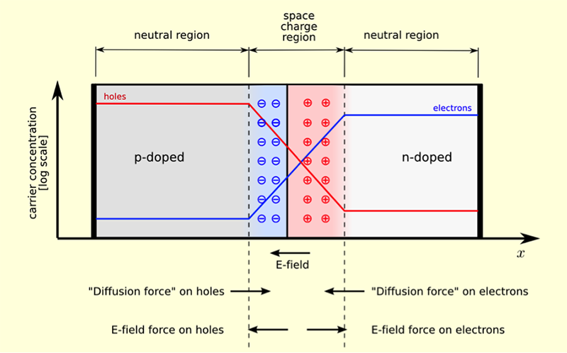
When light shines on the surface of the p-n material, photons excite electrons into conduction band, thus creating an electron-hole pair. If this happens in the n-doped side of the p-n junction, the newly excited electron is driven away from the junction, and the hole is swept across the junction to the p-doped side. This separation of the electron-hole pair is achieved by the action of the electric field in the space charge region. Then providing the external circuit (a wire) between the p- and n- semiconductors, we can initiate movement of the electron from the n-doped side to the p-doped side, where it recombines with a hole. This photo-induced electric current is the usable energy that can be harvested.
Please see the animated explanation to the light-induced current on the PVEducation website [49].
4.3. How PV performance is measured
4.3. How PV performance is measured
In the previous section, we understood how the photo-induced electric current is be generated at the p-n junction due to photovoltaic effect. How can we estimate the magnitude of that electric current?
To answer this question, first let us define the electron traffic across the band gap as generation or light-induced current (IL). Therefore, each photon absorbed is responsible for contributing one electron to the generation current inside the device. Hence, we can write:
where IL is light-induced generation current, q is the electron charge, N is the number of photons absorbed, and A is the surface area of the semiconductor exposed to light. Logically, we see that the more photons are absorbed, the higher the generation current. Also, the greater the area of semiconductor exposed to light, the higher the generation current. To be independent of the size of the cell, we can express this relationship in terms of current density (JL), which is current normalized by area:
For example, we can try to use this equation to estimate the current density of a photovoltaic device corresponding to the typical terrestrial light spectrum. Inputting values for electron charge (1.6 x 10⁻¹⁹ C) and number of photons in the absorbed range of spectrum for crystalline silicon (4.4 × 10¹⁷) to the above equation, we obtain:
(4.3)
This is the maximum current density that could be expected from a silicon cell, if there were no losses, and if all of the electrons were perfectly transferred through the external circuit. In reality, current losses take place, so the actual measured current density will be less than that ideal value (Markvart, 2000).
Next, let us see how the solar cell voltage can be estimated. The maximum voltage of a solar cell is determined by the semiconductor band gap. The electrostatic energy available due to separation of electrons and holes cannot exceed the band gap energy; otherwise, recombination would occur. The cell voltage (V) upper limit is therefore set by the following expression:
Numerically, the maximum voltage in volts is equal to the band gap energy in electron-volts. For example, the maximum voltage for a silicon solar cell is Vmax = 1.1 V
The same as with maximum current, the maximum voltage is never achieved practically because of losses and process limitations. However, in general, based on Eq. (4.4), the semiconductors with greater band gap indeed produce higher voltage (Markvart, 2000).
In summary: the maximum electric current of a solar cell is determined by the generation current, and the maximum voltage of a solar is determined by the material band gap.
In the above description, for simplicity, we assumed that all the photons (with energy above the band gap) reaching the surface are absorbed and transfer their energy onto electrons. This would be ideal and would give us ideal generation current. As a matter of fact, absorption of photos by semiconductors is material dependent and is controlled by the absorption coefficient. This is an important property to take into account, since it directly affects the charge carrier generation rate.
Reading Assignment
Absorption Coefficient / PVEducation.org [50]
Generation Rate / PVEducation.org [51]
The absorption coefficient role is well explained by these articles. Read through it to understand how the absorption coefficient affects the generation rate and how it changes with depth of the semiconductor material.
At this point, we have already recognized that the key parameters describing the performance of a solar cell are current density and cell voltage. We have looked into their origin - how they develop in the cell due to the photovoltaic effect, and looked at some factors that affect that process. Now, we will proceed to examination of the I-V characteristic (a.k.a. performance curve) and see how it is obtained and what different parts of this curve tell us about.
Using electric circuit notation, a solar cell can be represented by a diode, which represents the p-n junction.
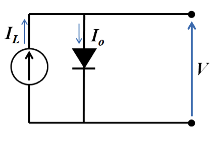
The current through the diode (Io) is the exchange current present when the element is in the dark. This is a small current compared to light-induced current (IL), which passes through the external load. The net current is the difference between the light and dark currents, or including Shockley diode equation:
where V is cell voltage, q is the charge of electron, k is the Boltzmann constant, and T is absolute temperature. This is the main equation that describes the relationship between voltage and current in the solar cell in operation. If we plot the cell voltage versus current (or current density), we will obtain the curve that generally looks like this (Figure 4.5):
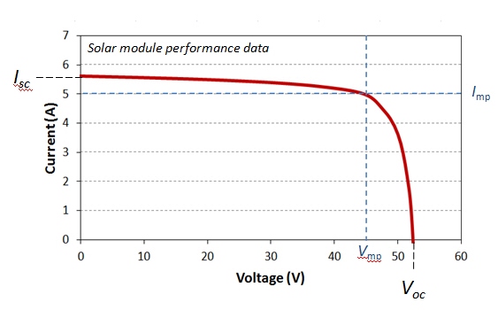
There are several important conditions to note on this curve. We see that at current being zero, the cell has the highest voltage. Because there is no current, the cell does not produce any work, but the voltage magnitude indicates the potential of the cell to do work. This is the open circuit voltage (Voc or OCV). The OCV is a very important characteristic of any galvanic cell (including solar cells), and it depends on the cell material. By re-arranging equation (4.5), and setting the net current to zero, we can express the open circuit voltage as follows:
At cell voltage set to zero, the cell current reaches some maximum limiting value, which is called short-circuit current (Isc). This is the kinetic parameter that shows the maximum current the cell is able to generate. It depends on the number of photons being absorbed by the material, optical properties of the cell and its size. You can imagine that if the sunlight intensity decreases for any reason, we will see a decrease in the short circuit current for a particular device. In an ideal case, the short-circuit current is equal to light-induced current: Isc = IL.
At any point on this curve (in Figure 4.5), we can define power output as follows:
At some point, the power will reach its maximum point, and the current and voltage corresponding to that point are defined as maximum power voltage (Vmp) and current (Imp):
These parameters are shown in the diagram in Figure 4.5. by blue dashed lines. They characterize the conditions when the cell produces the highest power output. This point is important because it is where the cell efficiency is usually determined.
At the maximum power point, we can also define the characteristic resistance of the cell (Rch). If the resistance of the external load is equal to Rch, then the maximum power is transferred to the load. The characteristic resistance can be determined from the Ohm's law:
The next term we need to define, when talking about the cell power output is the fill factor (FF). Please refer to the following reading to learn about the fill factor.
Reading Assignment
Fill Factor / PVEducation.org [52]
You are also welcome to try the FF calculators provided, which utilize the equations described on that website.
As you should have noted from the reading, the fill factor can be calculated as follows from the cell performance parameters:
The fill factor is a convenient metric to characterize the solar cell performance. For cells that work well, FF>0.7. Typical parameters of the single-crystal silicon solar cell are (Kalogirou, 2009):
Jsc = 32 mA/cm2
Voc = 0.58 V
Vmp= 0.47 V
FF = 0.72
Pmax = 2273 mW
Based on equation (4.10), the maximum power output of the PV system can be readily found using equation (4.11) if we know open-circuit voltage, short-circuit current, and fill factor.
The I-V characteristic is a convenient tool to explore the effect of various external variables on the cell performance. What is going to happen to a module output if temperature rises? What if light intensity drops because of the clouds? If cell is damaged or has bad contact with current collectors, how will it be reflected on the performance curve? Learn about these effects from the following readings:
Reading Assignment
Each of the following links will take you to a PVEducation web page that describes a certain effect on the solar cell performance. Read and take a note what events during the cell operation can cause these negative (parasitic) or positive effects (PVEducation.org).
Effect of Light Intensity [54]
Effect of Resistance [55]
Check Your Understanding - Question 4 (Essay)
Find the characteristic resistance of a solar cell that displays voltage of 40 V and current of 4 A at the maximum power point.
Rch =
Check Your Understanding - Question 5 (Essay)
Find the maximum power output of a PV system, if the open circuit voltage is 0.6 V, the short-circuit current is 0.32 A, and the fill factor is 0.8.
Pmax=
Check Your Understanding - Question 6 (Multiple Choice)
4.4. PV systems across scale
4.4. PV systems across scale
As we understand from the previous sections of this lesson, the electricity output of a single solar cell is relatively small, so cells need to be combined to provide enough power for any applications. Cells can be connected in series or in parallel. For example, when two identical cells are connected in parallel, the voltage of the system remains the same as for a single cell, but the current is doubled. When the same two cells are connected in series, voltage is doubled, while current remains the same. Examples of these combinations are shown in Figure 4.6.
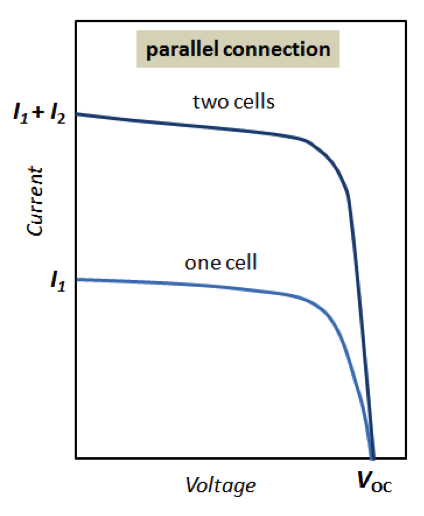
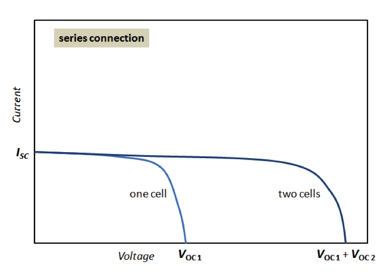
To provide significant power output, solar cells are typically grouped into modules. A module is an engineered system consisting of multiple solar cells, wiring, frame, and glass. A module is a typical commercial stand-alone unit for solar cell applications. Each module can consist of a variable number of cells arranged in two-dimensional structure (Figure 4.7). In one direction, cells are connected in series to a branch. Then several branches are connected in parallel to complete a module (Figure 4.7).
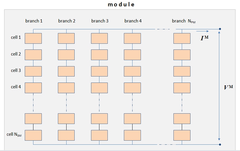
In Figure 4.7, the module voltage is denoted VM and module current is denoted IM (respectively, the single cell voltage and current will be denoted VC and IC in this presentation). This scheme depicts an example module that consists of NSM single solar cells connected in series and NPM parallel branches (subscript SM stands for series connection within module, and PM - for parallel connection within a module). The modules differ in design and may have variable number of parallel branches in order to deliver a certain current level. Many commercial modules may have simply one branch, i.e., all cells connected in series. To describe the electrical performance of a solar module, we can look at the model described in the reading material referred below. The model allows estimating the generated current and voltage of a module based on I-V characteristics of single cells.
Probing Question
Why would cells be normally connected in series, not in parallel, within modules?
If all the cells were connected in parallel, then the module would have an open circuit voltage of only 0.6 V, and a short circuite current of, for example 100 A. To transport this current, one would need an extremely thick cable. Furthermore, PV plants would need much higher voltages to be compatible with the grid.
The next step up the size scale will be grouping modules into an array (the same as it was done with grouping single cells into a module). A number of modules are connected in series within each branch, and then several branches are connected in parallel to form an array. Arrangement of modules in an array is shown in Figure 4.8.
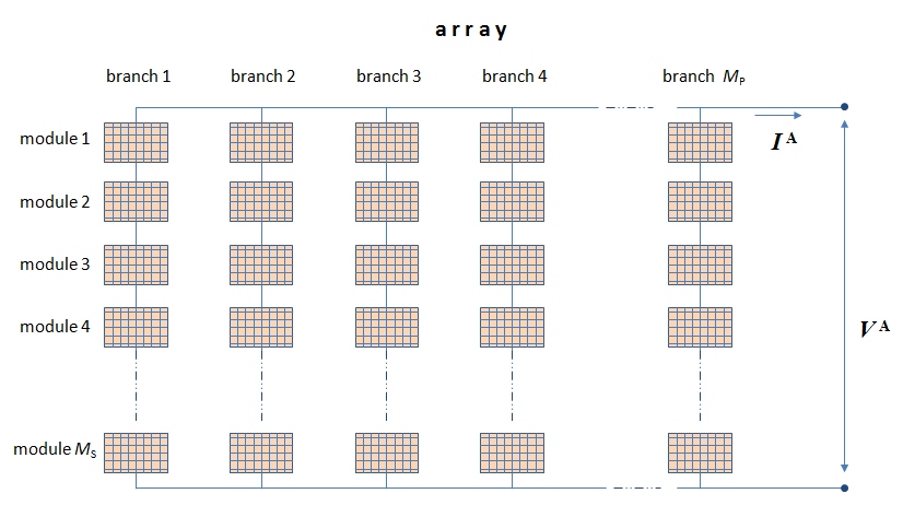
In Figure 4.8, each element is essentially a thumbnail of the arrangement shown in Figure 4.7. The total array current is IA depends on how many branches the arrays has, and the array voltage VA depends on how many modules are connected in one branch. Modules are common at the scale of distributed power generation (e.g. rooftops) and are also used as unit elements of larger solar facilities. Arrays are more typical for utility scale solar farms and plants. Next, you will learn how to calculate the voltage and current for large arrangements and thus to estimate the order of magnitude of power output.
Proceed to the following reading to become familiar with the basic models that describe the performance of solar modules and arrays.
Reading Assignment
Book Chapter: Kalogirou, S.A., Solar Energy Engineering. Processes and Systems. Elsevier, 2009, Chapter 9. "Photovoltaic Systems," pp. 482-486. (See E-Reserves via the Library Resources tab.)
Answer the following self-check questions to assess your learning of this section.
Check Your Understanding - Questions 7 & 8 (Multiple Choice)
Check Your Understanding - Question 9 (Essay)
What would be the voltage of the 5x5 module (consisting of the 5 parallel branches 5 single cells each connected in series), if each cell produces voltage of 0.4 V and current of 0.2 A?
V(module) =
I(module) =
4.5. Types of PV technology and recent innovations
4.5. Types of PV technology and recent innovations
There are different types of photovoltaics, some developed long ago, and others that are relatively new. Descriptions below provide a brief overview of a few well-developed PV materials. As you read through, please also open the links within each paragraph to get more information about each technology.
Monocrystalline silicon
Monocrystalline silicon solar cells are probably the oldest type of solar cells. They are made from pure silicon crystal, which has continuous lattice and almost no defects. Its properties provide for high efficiency of light conversion (typical ~15%; recent developments by SunPower boast improved efficiencies up to 22-24% ). Manufacturing of the Si crystals is rather complicated, which is responsible for high cost of this type of photovoltaics. Recent developments have decreased the total thickness of Si material used in monocrystalline cells to reduce cost. The monocrystalline silicon cells have a typical black or iridescent blue color. The monocrystalline silicon cells are believed to be very durable and last over 25 years. However, their efficiency will gradually decrease (about 0.5% per year), so replacement of operating modules might be needed sooner. The main disadvantages of the monocrystalline silicon panels are high initial cost and mechanical vulnerability (brittle). (Solar Facts and Advice: Monocrystalline Silicon [56], 2013)
Polycrystalline (or multicrystalline) silicon
Polycrystalline cells are made by assembling multiple grains and plates of silicon crystals into thin wafers. Smaller pieces of silicon are easier and cheaper to produce, so the manufacturing cost of this type of PV is less than that of monocrystalline silicon cells. The polycrystalline cells are slightly less efficient (~12%). These cells can be recognized by their mosaic-like appearance. Polycrystalline cells are also very durable and may have a service life of more than 25 years. The cons of this type of PV technology are mechanical brittleness and not very high efficiency of conversion. (Solar Facts and Advice: Polycrystalline [57], 2013)
Amorphous silicon (Thin-film)
Thin film photovoltaic cells are produced by depositing silicon film onto substrate glass. In this process, less silicon is used for manufacturing compared to mono- or polycrystalline cells, but this economy comes at the expense of conversion efficiency. Thin-film PV have efficiency of ~6% versus ~15% for single crystal Si cells. One way to improve the cell efficiency is to create a layered structure of several cells. The main advantage of the thin-film PV technology is that the amorphous silicon can be deposited on a variety of substrates, which can be made flexible and come in different shapes and therefore can be used in many applications. The amorphous silicon is also less prone to overheating, which usually decreases the solar cell performance. Amorphous silicon is most developed among the thin-film PV. (Solar Facts and Advice: Thin Film [58], 2013)
Figure 4.9, below, shows the trend of development and commercial implementation of different types of silicon PV technologies. There is no clear domination of a specific type of silicon substrate, as they all present a trade-off between cost and efficiency.
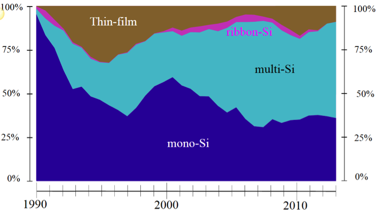
Cadmium Telluride, CdTe (thin-film)
CdTe PV are another kind of thin-film solar technology. It has become quite popular due to the lower cost per kW-hour. The best efficiency obtained with CdTe cells is around 16%. One of the advantages of the CdTe cells is that they capture shorter wavelengths of light than silicon cells can do. There are some environmental concerns related to the limited supply of tellurium and potential toxic impact of cadmium at the stage of CdTe panel disposal. Developing effective closed-loop recycling technologies can be a game-changing factor in favor of this technology. (Solar Facts and Advice: Cadmium Telluride [60], 2013)
Copper Indium Gallium Selenide (CIGS)
CIGS PV have become a popular new material for solar cells, as it does not contain toxic Cd, and has higher efficiency (just under 20%). At this moment, the CIGS are the most efficient among the thin-film PV technologies. While lab results confirmed high promise of this kind of photovoltaics, the mass production of CIGS proved to be a problem. The CIGS cells are manufactured by thin film deposition on a substrate, which can also be flexible (unlike the silicon cells). Similar to CdTe cells, the CIGS cells demonstrate good resistance to heating.
Polymer and organic PV
Organic materials are quite attractive since they can be involved in high-output manufacturing and also because they can be made in various thicknesses and shapes. These types of cells are relatively lightweight (compared to silicon cells). Also, they offer flexibility and relatively low fabrication cost. They, however, are much less efficient (about 1/3 of a typical Si cell efficiency) and sometimes prone to quicker degradation (shorter service life). More technical details about this type of PV technology can be read in this Wikipedia article: Organic Solar Cell [61].
These are a few most well-known varieties of PV technology, but there are many more innovations that are at the research and development stage. Breakthrough in new materials and cell design may be responsible for the growth of the PV industry in the upcoming decades. For this lesson discussion forum, you will be asked to do a search of recent innovations and share a quick synopsis of one that you believe especially interesting.
Summary and Activities
Summary and Activities
This lesson intended to provide you with the key concepts and terminology on the photovoltaic light conversion. It covers the basics of the photovoltaic effect and physical phenomena behind it, although it does not go into the depth of the science, but rather focuses on the practical understanding. Materials in this lesson also provide explanation to how the performance of the solar systems - cells, modules, arrays - is measured. Now, you should have an idea what the main parameters of the solar cell performance are, how to obtain them, and interpret them. You have learned how some of the key environmental parameters, such as temperature, light intensity, etc., affect the PV cell performance. The question of combining PV cells into bigger systems is discussed and illustrated with some examples, and we will return to the analysis of the larger-scale solar systems in Lesson 6, when more details will be given.
| Type | Description/Instructions | Deadline |
|---|---|---|
| Discussion Forum | Search recent research articles, press releases, and other sources for recent innovations in photovoltaic technology. Introduce this innovation at the discussion forum. In your post, try to deliver answers to the following questions:
|
Please submit your post by Sunday night. Responses are due by the following Wednesday. |
| Reading Quiz | Complete Lesson 4 Activity Quiz. | Please submit this assignment by next Wednesday night. |
References for Lesson 4
Markvart, T., Solar Electricity, John Wiley & Son, 2000.
Kalogirou, S.A., Solar Energy Engineering. Processes and Systems. Elsevier, 2009.
Honsberg, C. and Bowden, S., PVEducation.org, Photovoltaic Education Network., 2013.
Lesson 5: Concentrating Photovoltaics
Overview
Overview
Concentrating photovoltaic systems use lenses or mirrors to concentrate sunlight onto high-efficiency solar cells. Light concentration increases the flux of photons to the surface, which increases the photovoltaic current dramatically and opens ways to raise the conversion efficiency. There are predictions that concentrating photovoltaics (CPV) will be the next big trend in solar technology, although the price of electricity delivered by CPV systems is still too high to be commercially competitive. In this lesson, we will study the principles of concentrating photovoltaic systems and see how the concentration affects different parameters of solar cells. Also, we will review materials used for manufacturing concentrating photovoltaics. Finally, in this lesson, we will turn to the examples of recently commissioned CPV plants, some of them reaching the scale of multi-megawatt power generating facilities.
Learning Objectives
By the end of this lesson, you should be able to:
- understand and explain the principle of concentrating photovoltaics (CPV);
- analyze the effect of light concentration on PV cell performance;
- discuss examples of CPV applications on utility scale.
Readings
Cotal H. et al., III-V multijunction solar cells for concentrating photovoltaics, [62] Energy Environ. Sci., 2009, 2, 174–192
Montgomery, J., CPV Outlook: Demand Doubling, Costs Halved by 2017 [63], Renewable Energy World, Dec 12, 2013. Available from: Renewable Energy World [64]
Wesoff, E., Biggest CPV Plant in US Now on the Grid at Alamosa [65], GreentechSolar, May 15, 2012. Available from GreentechSolar [66]
5.1. What are concentrating photovoltaics?
5.1. What are concentrating photovoltaics?
One of the ways to increase the output from the photovoltaic systems is to supply concentrated light onto the PV cells. This can be done by using optical light collectors, such as lenses or mirrors. The PV systems that use concentrated light are called concentrating photovoltaics (CPV). The CPV collect light from a larger area and concentrate it to a smaller area solar cell. This is illustrated in Figure 5.1.
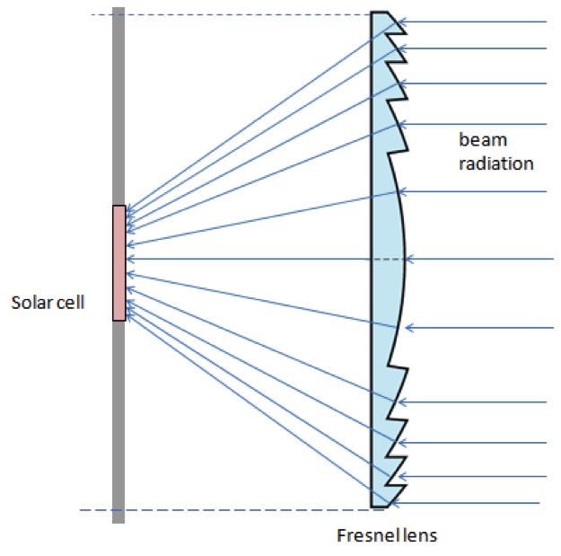
Lower efficiency CPV technologies may employ silicon, CdTe, and CIGS (copper indium gallium selenide) cells, but the highest efficiencies can be achieved with multi-junction cells. Field efficiencies for these multi-junction cells are in the 30% range, and laboratory tests have achieved upwards of 40% efficiency (Kurtz, 2011).
The CPV can only use direct beam radiation and cannot use diffuse radiation (diffused from clouds and atmosphere). Therefore, these systems are suited best for areas with high direct normal irradiance. For proper light concentration, sun tracking is needed for achieving high cell performance. Tracking is especially critical for high concentration systems. In general, the CPV can be classified into low-concentration, medium-concentration, and high-concentration.
| Low-concentration | Medium-concentration | High-concentration | |
|---|---|---|---|
| Concentration ratio | 2-10 | 10-100 | 100-400 (and above) |
| PV materials | Silicon | Silicon, CdTe, etc. | Multijunction cells |
| Cooling | not required | Passive cooling | Active cooling |
| Tracking | not required | 1-axis tracking | 2-axis tracking |
The high concentration of sunlight achieved with multijunction cells requires more sophisticated cooling and tracking systems, which can potentially result in higher energy costs.
CPV technology is expected to grow and to expand on market. The cost effectiveness of CPV technology is related to the fact that much smaller sized solar cells are used to convert the concentrated light, which means that much less expensive PV semiconductor material is used. Also, the optics added to the system are made from glass and are usually less expensive than the cells themselves.
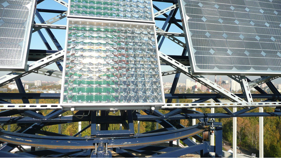
| Advantages | Disadvantages |
|---|---|
| Less PV material, hence less cost | With concentrated sunlight, formation of hot spots is possible |
| Increased efficiency | Tracking systems increase complexity |
| Higher productivity throughout the day due to tracking | CPV can properly function only under direct beam radiation |
CPV systems can produce significantly increased temperature on the surface of the PV material, so the energy should be distributed evenly over the cell area to avoid local overheating (hot spots), which can damage the material. Also, the thermodynamic efficiency of the photovoltaic conversion is less at elevated temperatures, so some kind of cooling may be beneficial. Active or passive cooling can be used. For the CPV cells with low and medium concentration ratios, active cooling is not necessary, since the temperatures reached are moderate. The high-concentration cells require high-capacity heat sinks to avoid thermal destruction of the materials.
5.2. Light concentration effect on PV performance and efficiency
5.2. Light concentration effect on PV performance and efficiency
Let us find out how the concentration of light affects the I-V characteristics of a solar cell. We remember from Lesson 4 that the generation current of a solar cell (IL) is a function of number of photons (N) hitting the photovoltaic surface:
where q is the electron charge, and A is the surface area of the cell. When light is concentrated, the number of photons increases according to the optical concentration ratio, so does the cell current. So, for the short circuit current of a solar cell (Isc), we can write:
where Copt is the optical concentration ratio (its definition was covered in Lesson 3). For convenience, we can denote cell performance parameters at concentrated light with an asterisk:
This equation essentially shows how much the cell short circuit current will change when the available light is concentrated Copt times. Then, we can substitute this equation to the I-V characteristic equation, which describes the cell performance over ranges of voltage and current:
where Voc* is the open circuit voltage (at concentrated light), k is the Boltzmann constant, T is the absolute temperature, and Io is the dark saturation current. Now, we are going to modify this equation because we want to find how the open circuit voltage at concentrated light would be related to the open circuit voltage at ambient light. We know that the short circuit current is the highest current a solar cell can show, while the dark current is a very low number, so the quotient in the parenthesis should be much greater than 1, and therefore, a simplified form of Equation (5.4) should be true:
Next, this equation can be modified by extending the natural log as follows:
The second term here is equal to Voc - the open circuit voltage without concentration, so we can write finally:
From Equation (5.7), it is obvious that there is logarithmic dependence between the cell open circuit voltage and the light concentration ratio. For example, if Copt = 10, the (kT/q)lnCopt term would be equal to 60 milivolts at 25oC - this is by how much the cell voltage will increase with tenfold light concentration. In case of higher concentration, for example, Copt = 1000, the voltage increase would be expected to be closer to 178 mV at 25 °C, which is relatively modest compared to current increase.
To estimate the concentration effect on maximum power output, we will use the equation (which was introduced in Lesson 4):
Substituting here Equations (5.3) and (5.7) and re-arranging, we obtain:
\[P_{\max }^* = {P_{\max }}{C_{opt}}\left( {1 + \frac{{kT}}{q}\frac{{\ln {C_{opt}}}}{{{V_{oc}}}}} \right)\]Self-Check Question 1
A solar cell generates maximum power of 2.3 W at regular light conditions at 25 °C. The open circuit voltage is measured at 0.55 V. Can you apply Equation (5.9) to estimate the maximum power of the solar cell if the light is concentrated 10 times (Copt = 10)?
As you can see, the cell power can raise dramatically because of light concentration, mainly because the cell current is significantly increased.
From the maximum power equation, we can further derive the effect of concentration on cell efficiency:
In this equation efficiency, (η) is expressed as the ratio of maximum cell power output to the irradiance on the cell surface. So, for concentrated light, the irradiance will be amplified to G* (which is proportional to Copt). The maximum power output at the concentrated light, Pmax, can be expressed as Voc*Isc*FF according to equation (4.9) in Lesson 4. Therefore, the expression for efficiency at the concentrated light can be modified as follows:
The algebraic transformation above is done by substituting Equations (5.3) and (5.7) into the equation (you can check). As a result, we see how "concentrated" efficiency (η*) is related to "non-concentrated" efficiency (η) through the optical concentration ratio. Try to apply this equation to find out what happens with the efficiency if you concentrate light ten times:
Self-Check Question 2
A solar cell has efficiency of conversion 15% at 25 oC (298 K). Open circuit voltage of the cell is 0.55 V. What efficiency ideally can we expect from it, when light is concentrated ten times (Copt = 10)? Use equation (5.11) and type your number (in percent) below:
As you can see, the efficiency of the solar cell increases slightly in concentrated light, but this increase is not as apparent as for absolute output parameters (e.g. power). This is because in efficiency we always consider a ratio of the output to input energy. Both output and input energies increase due to concentration, so based on Eq. (5.10) the efficiency does not change much. Moreover, the efficiency of real solar cells cannot increase indefinitely because of power losses to heat. The amount of those losses is determined by the cell series resistance (Rs). The higher the series resistance, the bigger the power losses:
Because the current flowing through the cell is proportional to the light concentration ratio, the power wasted can be presented as:
The power loss will grow very rapidly as the concentration ratio increases because of the exponent factor. So, there is no sense to increase concentration infinitely because those efforts may not pay off in terms of useful power increase. According to some studies (Luque, 1989), there is an optimum concentration ratio for each type of cells. It is pretty much dictated by the cell series resistance and can be expressed as follows:
Example
We are going to use Equation 5.14 to estimate the optimal concentration ratio for a solar cell of internal series resistance of 0.01 Ohm and producing short circuit current of 150 mA (at regular light).
The factor (kT/q) at 25 °C will be equal to 0.026 V, so for the optimal concentration, we can write:
That means that concentrating light at much greater than x17 ratios becomes unfeasible because of excessive losses.
Many solar cells designed for concentrated light in fact have special features to reduce the series resistance, but the limits of design may still be dependent on the cell material. For silicon, for example, it is hard to create cells that would be efficient at concentration ratios higher than 200 (Markvart, 2000).
5.3. Advanced materials for CPV
5.3. Advanced materials for CPV
Traditional PV systems use a large amount of silicon; in contrast, CPV systems use a small amounts of high‐efficiency PV materials. A typical example of such high-efficiency cells employed in high concentration CPV systems is a multijunction cell. The term multijunction refers to the cell structure, which has multiple p-n junctions combined within a single cell. Each junction is responsible for absorbing light within a particular wavelength range. All the junction currents are then combined to one output.
Combination of multiple p-n junctions within one cell is achieved by blending several semiconductor materials in layers or in other heterostructural formations. Manufacturing those formations can be tricky, and therefore costly. However, the pay-off on the efficiency side of the technology proves to be worthy. While single junction PV cells have the maximum theoretical efficiency around 34%, multiple junction cells can achieve in ideal case the limiting efficiency of 86.8% under concentrated sunlight (Wikipedia, Multijunction PV cell).
Consider the two single junction cases below (high band gap and low band gap) (Figure 5.3.1 and 5.3.2).
.png)
.png)
Figures 5.3.1 & 5.3.2 show two scenarios that illustrate the use of low band gap (top) and high band gap (bottom) materials. They both have limitations, which are responsible for low efficiency of single-junction PV cells. This is why tuning the different bandgaps to different components of light is a good idea in terms of minimizing power losses. Specific disadvantage of each scenario is stated under the plots. Combining different materials with different band gaps allows the cell to absorb a wide range of wavelengths and thereby to reach the highest efficiency.
To combine different materials in the multijunction cell, certain requirements need to be met for lattice-matching, current matching, and providing high opto-electronic performance. Regarding the first requirement of lattice-matching, one needs to make sure that the lattice constants of materials included are close. If the mismatch is significant, intercrystal defects can lead to quick degradation of electronic properties. For current matching, ordering of semiconductor layers within the multijunction cell is done in such a way that high-bandgap materials are placed on the top of the "sandwich," while the low-bandgap materials are placed on the bottom (Figure 5.4). That allows the light with low energy (greater wave lengths) to transmit to the lower layers and to be usefully absorbed. This concept is demonstrated in Figure 5.4. In this design, the suitable bandgaps need to be chosen so that the currents generated at each p-n junction are matched. If, for example, one of the junctions produces much lower current, it will be detrimental to the total current of the cell (because the layers are connected in series).
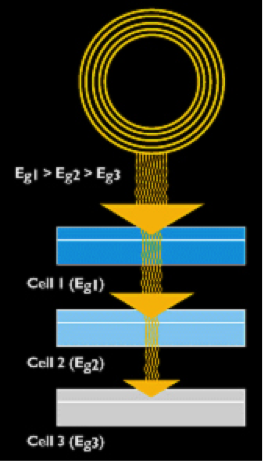
Check Your Understanding - Question 3 (Essay)
The configuration of layers shown in Figure 5.4 is logical in order to allow the maximum amount of light to be absorbed. What would happen if we accidentally put Cell 3 on top of the "sandwich"? Explain, then click for answer.
Next, we will refer to the following review on multijunction cell materials, their materials and design.
Reading Assignment
Journal Article: Cotal H. et al., III-V multijunction solar cells for concentrating photovoltaics, Energy Environ. Sci., 2009, 2, 174–192. [62]
Reading this article, note the basic principles of operation of multijunction cells and define the key parameters that are responsible for their high efficiency. The reading quiz in this lesson is largely based on this material.
Reading Quiz
Now it would be the best time to take the Reading Quiz. Go to Canvas Module 5 to complete the assignment.
5.4. CPV Market overview
5.4. CPV Market overview
CPV systems have been much less represented on market compared to traditional PV. In 2012, the only utility-scale CPV plant in operation was a 5 MW project in Hatch, New Mexico, (commissioned in June 2011) (Mendelsohn et al., 2012). However, the number of CPV projects launched for utility electricity production was rapidly growing. In 2012, CPV market was characterized by NREL as follows:
"The limited commercial success of CPV to date is partly due to the fact that these systems are more complex than PV systems. During 2008, as silicon prices were reaching new market highs, CPV systems appeared ready for a commercial breakthrough. Prices have since collapsed, however, and this has changed the economics of several alternative technologies, including CPV. Despite the dramatic decreases in silicon and conventional module pricing, the CPV market looks to be entering a tentative growth stage. According to NREL’s database, at least 10 utility-scale CPV projects, representing about 471 MW, are currently in development and hold long-term PPAs with utilities. San Diego Gas and Electric (SDG&E) holds the majority of these PPAs, both in terms of megawatts (410 MW, or 86% of total) and absolute numbers. One CPV project, the 30 MW Alamosa Solar Generating Project in Colorado, will be the largest CPV installation in the world when completed in 2012. Project developer Cogentrix received a DOE loan guarantee of $90.6 million in September 2011; this was the only loan guarantee awarded to a CPV project. Continued market growth for CPV will be the most important factor in keeping its costs competitive with traditional PV and with fossil fuels. Without manufacturing in the tens of megawatts per year, it is unlikely that CPV will achieve the cost reductions necessary to make it an economic technology, despite its high efficiencies" (Mendelsohn et al., 2012)..
Obviously, there is a certain degree of skepticism related to the economic viability of CPV utility-scale facilities, which currently rely on loans from government and investors. In spite of this fact, many energy analysts predicted fast growth of concentrated photovoltaics during the second decade of 21st century. The following web article talks about this trend based on some actual data.
Reading Assignment
Web Article: Montgomery, J., CPV Outlook: Demand Doubling, Costs Halved by 2017 [69], Renewable Energy World, Dec 12, 2013. Available from: Renewable Energy World
Check You Understanding Question 4 (Multiple Choice)
Check Your Understanding Question 5 (Essay)
Name some leading companies dealing with CPV installations mentioned in the article:
Check You Understanding Question 6 (Multiple Choice)
Check Your Understanding Question 7 (Essay)
Explain the Levelized Cost of Electricity (LCOE) metric.
Check You Understanding Question 8 (Multiple Choice)
Recent Updates
The above analysis and predictions were made seven years ago. Since then, PV market experienced rapid changes, and the rate and scope of those changes went beyond many predictions and proved to be disruptive to a number of current energy markets. CPV development has also been impacted. Let us take a look at a more recent NREL report that analyzed the status and promise of the CPV technology.
5.5. Ongoing activities and projects in CPV
5.5. Ongoing activities and projects in CPV
With the fast progress in research and development of concentrating photovoltaic technology, projects started to grow to implement CPV on the commercial scale. This section of the lesson introduces some examples of such implementations.
A summary of CPV projects now operating in the U.S. is given in Table 5.3 below. While CPV is less common in other world's locations, it would be worth to mention Golmud Plant [71] in China (2012-2013), with two phases adding up to 137 MW capacity and Touwsrivier CPV Project [72] in South Africa (2014), which is also one of the largest installations - 44.2 MW .
| Project | State | DNI (kWh/m2 yr.) | Land area (ha) | Company operating | Capacity (MW) |
|---|---|---|---|---|---|
| Alamosa Solar Project | CO | 2482 | 91 | Arzon Solar | 35.28 |
| Arizona Western College | AZ | 2628 | 1 | PPA Partners | 1.25 |
| Craftons Hill College | CA | 2263 | 3 | Craftons Hill College | 1.61 |
| Eubank Landfill Solar Array | NM | 2449 | - | Suncore PV Technology | 1.21 |
| Newberry Solar 1 | CA | 2650 | 10 | Soitec | 1.68 |
| Nichols Farms | CA | 2263 | 2 | Nichols Farms | 1.28 |
| Victor Valley College | CA | 2592 | 2 | Victor Valley College | 1.26 |
The Alamosa Solar Plant is one of the biggest project commissioned in the US, and represents one of the cover stories of CPV implementation. Some more details on this case are presented below.
Alamosa Solar Project
The Alamosa solar plant is located on 225 acres of land in Colorado and supplies electricity to the grid of the Public Service Company of Colorado. At the time of commissioning, Alamosa was the largest CPV plant in the world, but was later surpassed by the newly built plants in China. The plant boasts a set of the advanced controls to ensure grid efficiency. The loan issued on the project guarantees low risk profile, while it is clear that the CPV development still needs to provide lower electricity prices in the future to be long-term competitive with regular silicon PV and fossil fuel power plants. The news releases about the Alamosa plant are linked below.
Reading Assignment
Web Article: Wesoff, E., Biggest CPV Plant in US Now on the Grid at Alamosa, GreentechSolar [73], May 15, 2012. Available from GreentechMedia.
Web Article: Wesoff, E., Korean Utility Kepco Buys 30 MW Alamosa CPV Plant for $34M [74], August 30, 2016. Available from GreentechMedia.
Alamosa demonstrates the robustness and reliability of the Amonix CPV modules (Amonix 7700). The modules are grouped by seven into CPV systems (7 modules each). Every one of those systems has a separate inverter and controls.
Check out the design of the Amonix module in the following documents:
Summary and Final Tasks
Summary and Final Tasks
In this lesson, you learned about the special type of PV systems - concentrating photovoltaics. There are a few important features that make this technology attractive. They include:
- high efficiency of light conversion (reaching 40% and above based on some laboratory tests);
- small size of cells, which allows the use of less expensive PV materials;
- economic land use by CPV systems.
At the same time, sophisticated design, necessary for precise tracking and cell cooling, is responsible for higher cost of CPV systems and high price of electricity compared to regular PV or non-renewable power generation systems. The activities in this lesson are oriented towards understanding some fundamental parameters of PV and CPV system analysis.
The table below summarizes all activities that are due for this lesson. Some of those have been included in the body of the lesson, and this list simply repeats them for your reference.
| Type | Description/Instructions | Deadline |
|---|---|---|
| Reading Quiz/Reflection | This assignment presents you with a set of questions, which check your knowledge and understanding of some concepts discussed in the paper assigned for reading: Cotal H. et al., III-V multijunction solar cells for concentrating photovoltaics, Energy Environ. Sci., 2009, 2, 174. | Due date - next Wednesday |
| Written Assignment |
|
Due date - next Wednesday |
References for Lesson 5
Lesson 6: PV Power Conditioning
Overview
Overview
This lesson considers the principles of connecting solar cells to modules, and modules to arrays and larger systems for utility-scale electricity generation. To ensure the high-efficiency operation of an array or plant, a number of system components and pieces of equipment are needed. Here you will learn about some of those items and their purpose. Some of the designer's questions are: How do we put those components together and properly connect them? How do we select and match the electrical parameters of those components? What electrical and civil works are required to build a large scale PV plant? We will see how these questions are answered for different scales and different structural variations of photovoltaic systems.
For grid-connected PV systems, such parameters as voltage, current, and frequency should be matched to the ranges used by the grid. DC voltage may need to be stepped up or stepped down to match the grid requirements, and finally, DC power needs to be converted to AC power. All these steps constitute power conditioning, which is performed by an inverter - a special device that is responsible for seamless integration of solar power into the electric grid. In this lesson, we will learn about different types of inverters, their operation principle, their role, and conversion efficiency. The activities for this lesson will include a discussion forum and a reading quiz.
Learning Objectives
By the end of this lesson, you should be able to:
- explain basic strategies for the design of large scale PV plants;
- name the key components of PV systems and explain their purpose and basic principle of operation;
- list the main types of solar inverters and explain their role and efficiencies;
- discuss the key issues related to the connection of PV systems to the grid.
Readings
Book Chapter: Mertens, K. and Hanser, K.F., Photovoltaics: Fundamentals, Technology, and Practice, John Wiley & Sons, 2013. Chapter 6: Solar Modules and Solar Generators, pp. 133-159.
Book chapter: Mertens, K and Hanser K.F.,Photovoltaics: Fundamentals, Technology and Practice, Chapter 7: Photovoltaic System Technology, pp. 161-181.
Book Chapter: Komoto, K., Ito, M., van der Vleuten, P., Faiman, D., and Kurokawa, K., Energy from the Desert, Chapter 7. MW-Scale PV System Installation Technologies, pp. 86-98.
Industry Guide: "Inverters and PV System Technology (Industry Guide) [78]"Solarpraxis AG, Berlin, Germany, 2011.
6.1. Main components of large PV systems
6.1. Main components of large PV systems
The electric power generated by PV modules goes through a series of transformations before it reaches the grid. Those transformations specifically include adjustments of current and voltage, DC-AC conversion, and also distribution of power between storage and transmission paths. Cumulatively, we can call these operations power conditioning.
Power conditioning is an important function of any utility-scale solar plant, which ensures that the energy generated can be effectively and safely delivered to consumers. To accomplish the proper power conditioning, we need a number of specialized components (in addition to the PV modules), and we are going to take a closer look at some of those components and their operation principles in this lesson.
Photovoltaic plants contain a large amount of supporting equipment, which serves to balance the system and to make it sustainably operational. The extra components include inverters, controllers, transformers, wiring, connector boxes, switches, monitoring devices, charge regulators, energy storage devices - all of which help prepare electric power for utilization. PV systems are typically modular in design, so that additional sections can be added to the plant or removed for repairs without significant disruption of its infrastructure. The energy flow at the solar plant runs through a variety of devices, which are connected by wire network and related hardware. This supporting infrastructure is often referred to as balance of system (BOS). The quality of the BOS is very important for providing lasting and efficient operation. The industry goal is to provide PV systems with an operational lifetime of at least 25 years. [Foster et al., 2010].
The general line-up of the key components of the BOS is illustrated in the generic system scheme below.
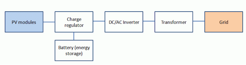
Let us briefly discuss the main components in this scheme and describe their functions.
Charge controllers or regulators manage the flow of electricity between the solar modules (arrays), energy storage, and loads. The appropriate charge control algorithm and charging currents need to be matched for the batteries (or other energy storage devices) used in the system. The main purposes of a charge controller is to protect batteries from damage and to prevent overcharging or excessive discharging. Typically, these devices operate in the switch on / switch off mode. For example, when the terminal voltages supplied from a PV system to the battery increases above a certain threshold value (Vmaxoff), the switch disconnects the PV array. The array is connected again when the terminal voltage drops below a certain value (Vmaxon). This hysteresis cycle protects the battery from overcharging. Similarly, charge controllers help prevent battery excessive discharging. When the current of the load connected to the battery is higher than the current delivered by the PV array, the load is disconnected as the terminal voltage falls below Vminoff and is connected again when the terminal voltage increases above a certain threshold Vminon. Charge controllers also participate in voltage conversion and maximum power tracking [Kalogirou, 2009].
Inverters - devices that convert DC power coming from the solar modules to AC power (necessary for grid) are critical components of any PV systems. Inverters convert DC power from the batteries or solar modules into 60 or 50 Hz AC power. As with all power system components, the use of inverters results in energy losses due to interferences. Typical efficiency of an inverter well matched to the array is around 90%. Inverters are key components in both grid-connected and distributed power applications, and usually are a significant part of system cost. The AC current produced by inverters can have square, modified sine, and pure sine wave output (Figure 6.2). The pure sine is high cost and has the best power quality. The modified sine is medium cost, but has less efficiency. The square wave is low cost and lowest efficiency, which is only used by some applications. Square wave signals can be harmful to certain electronics due to high-voltage harmonic distortion. Inverters are common sources of electromagnetic noise, which can interfere with sound and video equipment. So, the inverters boxes must be grounded according to the code requirement and safety reasons [Foster et al., 2010].
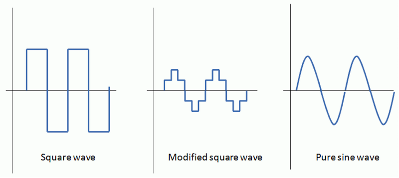
Grid-tied inverters are used to tie the PV system to the utility grid. They convert DC power to AC power in synchronization with the grid. For example, if grid fails for any reason, the inverter will shut down as well. The main considerations related to PV-grid interconnection include safety, power quality, and anti-islanding. Islanding is the condition when in case of power grid going down, inverter attempts to power the grid and can result in equipment damage and safety risks to technical personnel. Grid power line with PV modules connected to it is a typical islanding situation. After the grid is down, the PV panels still continue to power the line as long as the solar radiation is present. Thus, we have an "island" of powered line within un-powered grid. Most AC grid-ties inverters have anti-islanding feature, so the inverter will reduce power to zero within 2 seconds of the grid shut-down.
Inverters are rated by the total power capacity (from hundreds to a million watts). Some inverters have a good surge capacity for starting motors, but others may have limited surge capacity. So, designers should specify both type and size of the load to be connected to the inverter [Kalogirou, 2009].
DC-DC converters or transformers are used to step up (boost) or step down (buck) voltage of DC current. Therefore, the voltage of the solar array can be chosen independently of the voltage of the load. This kind of convenience comes with a cost - DC-DC converter always have losses, although the good models have efficiency as high as 95%, with some waste heat generated [Mertens and Hanser, 2013]. Ideally (if there were no losses):
\[{P_1} = {V_1} \times {I_1} = {V_2} \times {I_2} = {P_2}\]
Where V1 and I1 are voltage and current at the input (from solar module) and V2 and I2 are voltage and current at the output, respectively.
Batteries are used in many types of PV systems to supply power at low sun conditions (night or low irradiance). Additionally, batteries are required in solar systems because of the fluctuating nature of the PV output. The battery size/capacity is selected according to the load. They are usually connected in parallel to match higher capacity. There are several types of batteries commercially available for solar applications, including lead-acid, nickel-cadmium, nickel hydride, and lithium-ion. The main requirement for the batteries that are used as energy storage for solar systems is that they must be able to go through deep charging and discharging cycles without too much degradation. Batteries are classified by the nominal capacity (qmax), which is the maximum number of ampere-hours that can be extracted from the battery under certain standard conditions.
The efficiency of a battery can be defined as the ratio of the charge extracted during discharge to the amount of charge needed to restore that state of charge. The efficiency depends on State of Charge (SOC), which is the ratio between the present capacity of the battery and the nominal capacity (SOC = q/qmax). For example, SOC=1 when the battery is fully charged, and SOC=0 when the battery is fully discharged. The battery lifetime is often presented as the number of charge-discharge cycles the battery can sustain before losing 20% of its nominal capacity [Kalogirou, 2009].
Batteries used in power generating solar systems are actually different from car batteries. The car batteries are not designed to withstand the deep charge-discharge cycles and therefore should not be used with solar power generation. Batteries are usually installed in well-ventilated locations - (e.g., utility rooms) to minimize hazards from spills and made them available for easy maintenance or replacement. More details of energy storage technology will be covered in Lesson 9.
Grounding and bonding of related DC and AC circuits is important to maintain system integrity. According to the U.S. electric code, the systems operating under 50 V are not required to be grounded, although chassis grounding is required for all hardware.
6.2. Connections in large PV systems
6.2. Connections in large PV systems
Power output from the solar arrays would be dependent on the arrangement and connection of the modules within the plant and can be varied based on local preference. To know how we can manipulate power output, we need to understand the principles of interconnections of PV cells in the modules and connections of those modules to the direct current equipment. From the following reading, you will learn about different types of connections and how they determine the module response to disturbances such as shading or formation of hot spots. Additionally, we will see how the module performance may be affected by different environmental parameters, such as irradiance, temperature, and type of solar cell material. Finally, this reading will describe how the cable connections are made between the solar modules and a generator.
Reading Assignment
Book Chapter: Mertens, K. and Hanser, K.F., Photovoltaics: Fundamentals, Technology, and Practice, John Wiley & Sons, 2013. Chapter 6: Solar Modules and Solar Generators, pp. 133-159. (See E-Reserves via the Library Resources tab.)
Note: The quiz at the end of this lesson will include a few questions on this reading. Please refer to the Summary and Activity page for more details.
6.3. Architecture of the large-scale PV systems
6.3. Architecture of the large-scale PV systems
Development of large solar PV plants has been underway in a number of countries, especially where the government-backed incentives and legislation were in place to support renewables. Since 2000, installation of MW-scale PV systems has been initiated in Germany, Spain, Italy, Greece, and further taken into even larger scale in U.S., China, India, and Brazil. The trend really picked up after 2007, when the number of the more than 1 MW systems grew from 20 to over 100 within a few years. Industry experts predict that the trend will hold and perhaps even accelerate into the future as the demand for renewable energy resources escalates. The average and maximum size of the utility solar plants (typically 5 MW to 500 MW) increases as well. The Topaz Solar Farm, located in San Luis Obispo County, California, is one of the largest solar photovoltaic power plant in the U.S. (Figure 6.3). This facility has the capacity to generate 550 megawatts (MW) of solar electricity using 5 million panels.
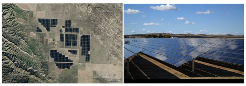
Credit: Pacific Southwest Region via Wikimedia [79]
The list of the world's largest PV plants [80] is updated from year to year, and you can see that Topaz benchmark has been already beaten repeatedly now, and the top facilities currently exceed GW limit. One of the attractive factors of the utility PV plants is that those facilities can be built relatively quickly (within 6-12 months) due to modular structure, unlike major hydroelectric, geothermal, or fossil fuel facilities, which would be typically developed over 3-5 year span. This presents a great opportunity for emerging economies to effectively meet their growing energy demands, especially since many of those countries possess an excellent solar resource.
Initially, the PV plant design is developed at the stage of feasibility assessment, which includes estimation of solar resource and expected yield. Then, the plant design is further improved, taking into consideration other local limitations and constraints. The feasibility stage also includes site measurements, topography mapping, environmental setting assessment, and social impacts. Key design features include such technical information as PV module type, tilting angle, mounting and tracking systems, module arrangement, and balance of system (BOS) components - inverters, connections, switches, and storage solutions. Further optimization of plant design would deal with such issues as shading, performance degradation, and economic trade-offs between increased complexity and energy yield.
The design of a utility scale PV plant is a complex endeavor. With many available choices of components and options for optimizing performance, it is important to strike a balance between cost savings and quality. Engineering decisions require significant technical expertise and should be "informed" decisions based on both optimization models and practical experience.
The following reading will introduce the main principles of the design of very large PV systems.
Reading Assignment
Here you will have a chance to study different aspects that need to be considered during the PV plant design and construction. Advances in system architecture, civil works, operational regimes allow significant cost reductions and better marketability of the solar energy in those regions.
Komoto, K., Ito, M., van der Vleuten, P., Faiman, D., and Kurokawa, K., Energy from the Desert, Chapter 7. MW-Scale PV System Installation Technologies, pp. 86-98.
Abbreviations in the reading:
- VLS-PV - very large scale photovoltaic
- PCU - power conditioning unit
- MVA - megavolt ampere
- DC - direct current
- AC - alternate current
- IGBT - insulated gate bipolar transistor
- EPC - engineering, procurement, construction
Following this reading, please take the reading quiz in Canvas (see Module 6).
6.4. Inverters: principle of operation and parameters
6.4. Inverters: principle of operation and parameters
Now, let us zoom in and take a closer look at the one of the key components of power conditioning chain - inverter. Almost any solar systems of any scale include an inverter of some type to allow the power to be used on site for AC-powered appliances or on the grid. Different types of inverters are shown in Figure 11.1 as examples. The available inverter models are now very efficient (over 95% power conversion efficiency), reliable, and economical. On the utility scale, the main challenges are related to system configuration in order to achieve safe operation and to reduce conversion losses to a minimum.

The three most common types of inverters made for powering AC loads include: (1) pure sine wave inverter (for general applications), (2) modified square wave inverter (for resistive, capacitive, and inductive loads), and (3) square wave inverter (for some resistive loads) (MPP Solar, 2015). Those wave types were briefly introduced in Lesson 6 (Figure 11.2). Here, we will take a closer look at the physical principles used by inverters to produce those signals.
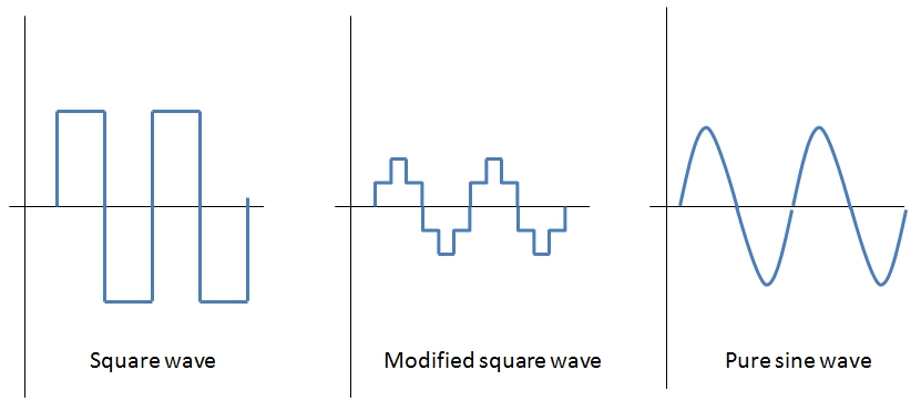
The process of conversion of the DC current into AC current is based on the phenomenon of electromagnetic induction. Electromagnetic induction is the generation of electric potential difference in a conductor when it is exposed to a varying magnetic field. For example, if you place a coil (spool of wire) near a rotating magnet, electric current will be induced in the coil (Figure 11.3).
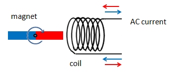
Next, if we consider a system with two coils (Figure 11.4) and pass DC current through one of them (primary coil), that coil with DC current can act analogously to the magnet (since electric current produces a magnetic field). If the direction of the current is reversed frequently (e.g., via a switch device), the alternating magnetic field will induce AC current in the secondary coil.
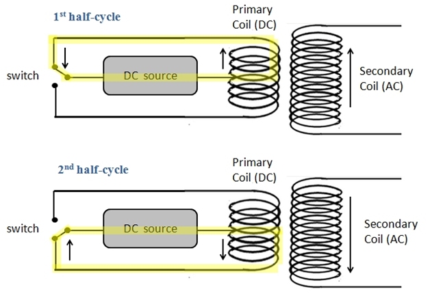
The simple two-cycle scheme shown in Figure 11.4 produces a square wave AC signal. This is the simplest case, and if the inverter performs only this step, it is a square-wave inverter. This type of output is not very efficient and can be even detrimental to some loads. So, the square wave can be modified further using more sophisticated inverters to produce a modified square wave or sine wave (Dunlop, 2010).
To produce a modified square wave output, such as the one shown in the center of Figure 11.2, low frequency waveform control can be used in the inverter. This feature allows adjusting the duration of the alternating square pulses. Also, transformers are used here to vary the output voltage. Combination of pulses of different length and voltage results in a multi-stepped modified square wave, which closely matches the sine wave shape. The low frequency inverters typically operate at ~60 Hz frequency.
To produce a sine wave output, high-frequency inverters are used. These inverters use the pulse-width modification method: switching currents at high frequency, and for variable periods of time. For example, very narrow (short) pulses simulate a low voltage situation, and wide (long pulses) simulate high voltage. Also, this method allows spacing the pulses to be varied: spacing narrow pulses farther apart models low voltage (Figure 11.5).
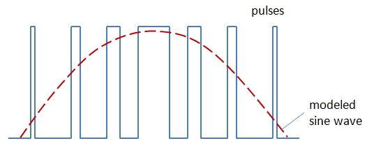
In the image above, the blue line shows the square wave varied by the length of the pulse and timing between pulses; the red curve shows how those alternating signals are modeled by a sine wave. Using very high frequency helps create very gradual changes in pulse width and thus models a true sine signal. The pulse-width modulation method and novel digital controllers have resulted in very efficient inverters (Dunlop, 2010).
6.5. Efficiency of Inverters
6.5. Efficiency of Inverters
The efficiency of an inverter indicates how much DC power is converted to AC power. Some of the power can be lost as heat, and also some stand-by power is consumed for keeping the inverter in powered mode. The general efficiency formula is:
where PAC is AC power output in watts and PDC is DC power input in watts.
High quality sine wave inverters are rated at 90-95% efficiency. Lower quality modified sine wave inverters are less efficient - 75-85%. High frequency inverters are usually more efficient than low-frequency.
Inverter efficiency depends on inverter load.
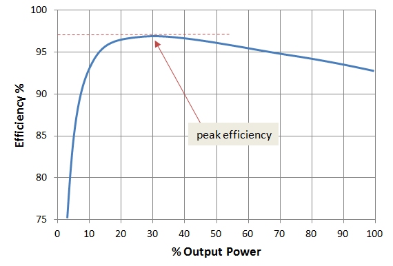
Figure 11.8. Typical generic inverter efficiency curve. Below 10-15% of power output, efficiency is quite low. At high output power, the efficiency is steadily high with some small variations.
The behavior in Figure 11.8 partially results from the fact that stand-by losses for an inverter are the same for all output power levels, so the efficiency at lower outputs is affected more.
There are three types of efficiency ranking used for inverters. You may come across those numbers as you research different models and manufacturers. Those three types are:
- Peak efficiency (shown by arrow in Figure 11.8) indicates the performance of the inverter at the optimal power output. It shows the maximum point for a particular inverter and can be used as a criterion of its quality.
- European efficiency is the weighted number taking into account how often the inverter will operate at different power outputs. It is sometimes more useful than peak efficiency, as it shows how the inverter performs at different output levels during a solar day.
- California Energy Commission (CEC) efficiency is also a weighed efficiency, similar to the European efficiency, but it uses different assumptions on weighing factors.
The main difference between the European and CEC efficiencies is that the assumptions about the importance of each power levels for a particular inverter are based on the data for Central Europe in the former case, and California in the latter. Hence, different formulae are used to calculate those values:
These methods of calculations need to be taken into account when using inverter specifications (Martin, 2011).
To learn more details about inverter efficiency, please go to the following reading.
Reading Assignment
Book chapter: Mertens, K and Hanser K.F., Photovoltaics: Fundamentals, Technology and Practice, Chapter 7, Section 7.2.4 Efficiency of Inverters, pp. 177-181.
Please answer the following self-check questions based on the above material.
Check Your Understanding
Question 1
What is the efficiency of an inverter that outputs 2000 W of AC power using an input of 2200 W of DC power?
Question 2
Question 3
See if you can estimate the European efficiency for an inverter that has the following efficiency curve data: at 5% power output η=85%, at 10% η=91%, at 20% - η=96%, at 30% η=97%, at 50% η=96%, and at 100% power η=95%. Input your value below, compare with the answer.
6.6. Switching devices
6.6. Switching devices
Switching function in inverters is needed to alternate the direction of the DC current in order to produce AC power. Usually, electronic semiconductor devices are used to perform switching, such as transistors and thyristors.
Thyristors are used in basic models of inverters. They have three leads and usually "switch on" in response to current applied to one of the leads. Thyristor have only two modes: ON and OFF, the same as mechanical switches. More details on thyristors can be found on this Thyristor Wikipedia Page. [82]
Transistors are similar in switching capability to thyristors, but they instead respond to voltage applied rather than current. That allows to smoothly vary the transistor's internal resistance. So in addition to ON and OFF functions, transistors also allow dimmer capability. More details on transistors can be found on this Transistor Wikipedia Page [83].
There are two main types of transistors used in solar inverters:
- Metal Oxide Semiconductor Field Effect Transistors (MOSFETs)
- Insulated Gate Bipolar Transistors (IGBTs)
The MOSFET type is suitable for very high switching speeds (up to 800 kHz), but operate at relatively low voltage. The IGBT type switch at lower speeds (below 20 kHz), but withstand higher voltage and high current (Dunlop, 2010).
Switching Control
Switching devices, such as thyristors and transistors, need to be controlled by an external signal. In the basic inverter designs, switching is controlled by the utility power line. Such switching devices are referred to as line-commutated. They are turned on and off by alternating half-cycles of the utility voltage, thus synchronizing the inverter output with grid line current. Although efficient, the line-commutated inverters have one disadvantage: they cannot operate independently of the grid.
Some inverters may contain an internal device that controls switching. Such a device is usually a microprocessor that provides precise timing. Such inverters are called self-commutated. Self-commutated inverters have additional capabilities of shaping the AC output and suppressing harmonics. And they can operate independent of utility power. There are two varieties of self-commutated inverters: voltage-source and current-source. They take the DC input as voltage source or current source, respectively, for conversion of the power to the AC output. Most of the present day inverters involved in solar plants are self-commutated (Dunlop, 2010).
6.7. DC/DC Conversion
6.7. DC/DC Conversion
A typical output voltage of PV panels can be on the order of 30 V, and it is too low for being converted to AC and fed to the grid. Therefore, DC/DC conversion is often a necessary step before the DC current from the PV system is supplied to the inverter. Most of the power conditioning units include some type of DC/DC converter. Direct current converter transforms the DC voltage V1 to DC voltage V2 via adjusting the current (I):
This is an ideal case, when input power is equal to the output power. In reality, there are always conversion losses, which lead to typical efficiencies in the range 90-95%.
DC/DC conversion allows keeping the voltage on the PV and voltage on the load separately controlled. There are two main types of DC/DC converters depending on the direction of voltage change: (1) boost converters transform smaller voltage to higher voltage and (2) buck converters transform higher voltage to lower voltage.
Please proceed to the following reading to learn more details about the operating principles of the DC/DC converters.
Reading Assignment
Book chapter: Mertens, K and Hanser K.F., Photovoltaics: Fundamentals, Technology and Practice, Chapter 7, Section 7.1.2 DC/DC Converter, pp. 161-168. (See E-Reserves via the Library Resources tab.)
MPP tracking
One of the important functions that DC/DC converting devices can perform is maximum power point (MPP) tracking. The idea behind it is to keep the solar power system operating constantly at the maximum power, i.e., at the voltage Vmp and current I mp. These parameters were discussed in Lesson 4, and Figure 4.4 illustrates the concept.
Assume that at a certain ambient irradiance, a solar cell or an array operate at the maximum power. Then, if the irradiance conditions change, the performance characteristic (I-V curve) of the cell changes (Figure 11.6). Thus, if the output voltage is kept constant, the output current drops significantly. The MMP tracker is used to adjust the voltage to the new Vmp value, thus maintaining the maximum power output.
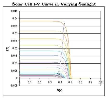
I-V performance curves of a solar cell in varying sunlight. The upper curves demonstrate the cell performance at higher irradiance conditions. The vertical path crossing the performance curves indicates the shift of the maximum power point.
In large solar facilities, it is beneficial to have an individual MPP tracking unit to be connected to each array output, since different arrays may have different I-V characteristics (due to varying irradiance, orientation etc.). This improves the overall performance of the plant.
An algorithm for MPP tracking is discussed in Section 7.1.3 of the above-referenced reading.
Please answer the following self-check questions before proceeding to the next section.
Check your understanding
Question 4. The principle of the buck DC/DC converter is based on periodically switching on and switching off the signal and then smoothing the output. Which parameter is used to regulate the switch-on/switch-off regime?
Question 5. Can you calculate the output of the boost DC/DC converter that uses the duty factor of 0.6 to convert 10 V of DC?
6.8. PV--Grid connection
6.8. PV--Grid connection
Interconnections in solar systems and their connection to the public grid are regulated by National Electrical Code®(NEC). The NEC is a nationally recognized standard for safe electrical installation and is routinely applied all over the U.S. It is intended for use by trained personnel and is applied to integration of all wiring, overcurrent protection, disconnects, grounding, and equipment regulations. Article 690 of NEC is specifically dedicated to solar photovoltaic systems, and article 490 is applied to large utility-scale systems (over 600 V). Importantly, the NEC addresses the circuit requirements for solar systems, such as maximum current and voltage.
Maximum Voltage Rating
The first condition for determining the maximum DC voltage is that it should be lower than the voltage limits defined for any component on the DC side of the system. The maximum DC voltage output (Vmax) from a PV system can be estimated using the following formula (Dunlop, 2010):
where Voc is the open circuit voltage of a module at 25 oC, nser is the number of modules connected in series, and CT is the temperature correction factor. The CT factors account for the voltage increase with decreasing temperature and can be found in Table 690.7 in Article 690—Solar Photovoltaic (PV) Systems [85] of NEC.
For Example
What would be the total maximum output voltage of the system including 20 modules connected in series, each module having open circuit voltage of 18 V, if the minimum expected temperature at the locale is -25 oC?
Applying the formula (11.1): Vmax = 18 V × 20 × 1.20 = 432 V
Maximum Current Rating
Per NEC code Article 690.8, which deals with circuit sizing and rating, there are two different PV circuits distinguished:
(1) PV source circuits - conductors between PV modules and to the common point of connection, i.e., junction box
and
(2) PV output circuits - conductors between the junction box and the inverter or DC loads
These two types of circuits are schematically shown in Figure 11.7. The PV source circuits and PV output circuits are rated differently with respect to the maximum current.
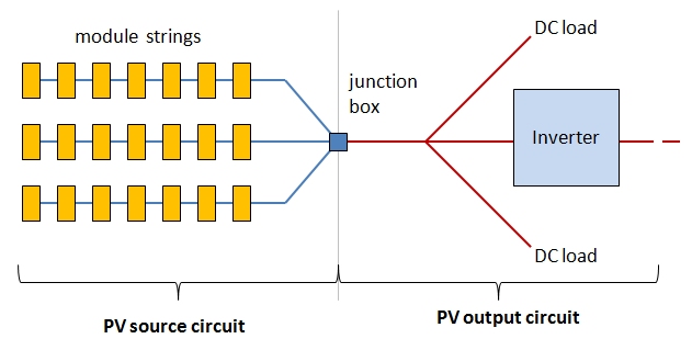
The maximum DC current rating for PV source circuits is considered at 125% of the sum of all short-circuit currents rating of all modules. This assumption is based on the fact that under enhanced irradiance conditions, modules can occasionally generate currents higher than nominal Isc values. The maximum source current is determined for each single string.
For example:
If the module short circuit current Isc = 4.8 A, then
Imax(source) = 4.8 × 1.25 = 6 A
The maximum DC current rating for PV output circuit needs to take into account all parallel strings, and in this case the source maximum current needs to be multiplied by the number of strings (npar) involved in the system.
For example:
If we have three parallel strings of modules (like shown in Figure 11.7), each with source maximum current of 6 A, then
Imax(output) = Imax(source) × npar = 6 A × 3 = 18 A
In summary, the cables within each string should be able to withstand currents of 6 A, but the cables on the inverter side should be ready for 18 A.
The estimates of the system maximum voltage and currents are key factors for choosing the inverters, determining wiring, conductor size, and required overcurrent protection.
Interconnection types
By the type of interconnections, there are several inverter types employed at different PV systems. They include stand-alone, interactive, and bimodal inverters.
The stand-alone mode does not involve grid connection, but rather uses the battery storage to collect the power from PV and convert it to AC for specific applications (Figure 11.8a). If the battery storage is depleted, the system becomes stressed.
The interactive mode does not use any energy storage, and the inverter serves as the interface between the PV and the utility grid (Figure 11.8b). In this case, power can flow in both directions. If the on-site power demand is higher than the amount supplied from the PV, the system can draw power from the grid. If the produced power is greater than the on-site power demand, the excess power is fed to the grid.
Finally, the bimodal connection (Figure 11.8c) combines both stand-alone and interactive options. Here, the energy storage provides backup for critical loads, while the excess power is fed to the grid, like in the interactive mode. If for any reason the grid loses power, this bimodal system uses a separate dedicated distribution panel to support the critical loads (such as computers, lighting, water pumping, etc.) (Dunlop, 2010).
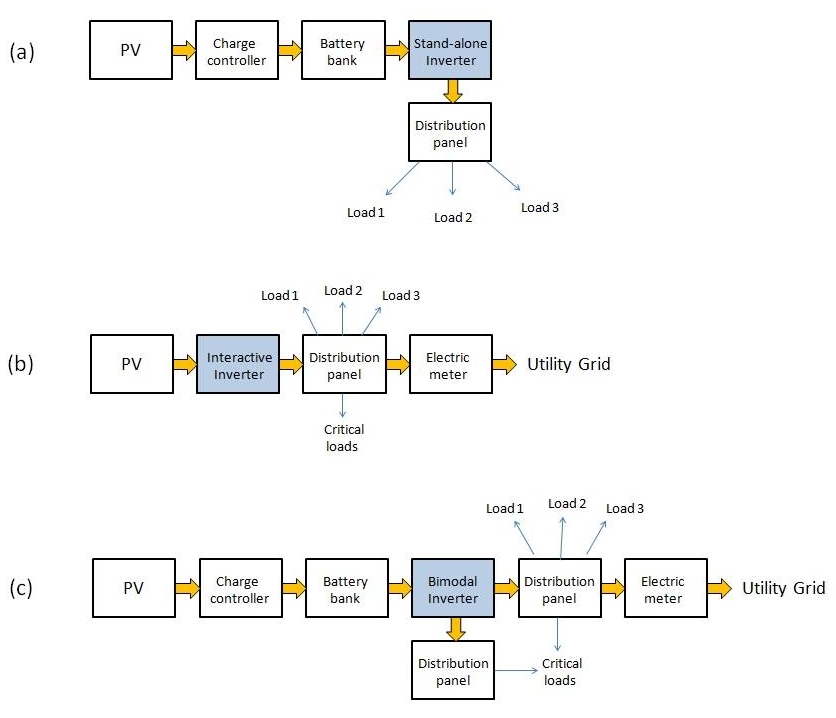
A. PV to charge controller to battery bank to stand-alone inverter to distribution panel (to load 1,2,3)
B. PV to interactive inverter to distribution panel (to load 1,2,3 & critical) to electric meter to utility grid
C. PV to charge controller to battery band to bimodal inverter (to distribution panel to critical load) to distribution panel (to load 1,2,3 & critical) to electric meter to utility grid
Please refer to the following reading to gain more insight in inverter operation in grid-connected systems.
Reading Assignment
Book chapter: Mertens, K and Hanser K.F., Photovoltaics: Fundamentals, Technology and Practice, Chapter 7, Section 7.2 Grid Connected Systems, pp. 168-177. (See E-Reserves via the Library Resources tab.)
Grid-connection challenges
The following are some known concerns arising from interconnection of different scale PV systems to the utility grid.
- Islanding is the condition when the solar power facility keeps supplying power to the grid during grid outage. This is a serious safety hazard, since utility workers who repair the grid may be exposed to unexpected voltage present in the utility line. To prevent damage to personnel and equipment, all grid-bound inverters must be able to detect outages and block power transfer. Inverters with such capability are referred to as anti-islanding inverters. Bimodal inverters may remain in stand-alone mode of operation while being disconnected from the utility grid line.
-
Power quality is reflected in the several electrical performance parameters, such as voltage, frequency, harmonic distortion, noise, etc. Many loads and equipment connected to the grid are designed to operate at certain prescribed conditions and may not be able to withstand voltage fluctuations and other disturbances. Low-quality inverters can cause poor power quality, which can cause damage to the sensitive equipment, or create hotspots in transformers.
-
Phase disbalance can occur if single-phase inverters are connected to three-phase power systems. Solution to the mismatch may be connection of three small inverters, each to a different phase, or employing a single three-phase inverter.
Please answer the following self-check questions before proceeding to the next section.
Check your understanding
Question 6. Will the PV cell voltage be higher or lower if the outdoor temperature drops to -10 oC? Find the temperature correction factor for this case.
Question 7. If a PV cell outputs 20 V at 25oC, what voltage can we expect from it at -10oC?
Question 8. Which of the following is usually true with grid-connected solar plants?.
Additional Reading on Inverters
Dunlop, J.P., Photovoltaic Systems, 2nd Ed., Chapter 8: Inverters. American Technical Publishers, 2010.
King, D.L., Gonzalez, S., Galbraith, G.M., and Boyson, W.E., Performance Model for Grid-Connected Photovoltaic Inverters [86], Sandia Report SAND2007-5036, 2007.
Summary and Final Tasks
Summary and Final Tasks
This lesson addresses multiple issues related to the scale up and deployment of photovoltaic technology. PV arrays generate DC power, sometimes a lot of it. It takes a lot of hardware and engineering effort to use that power safely and efficiently. Here, we looked into the principles of connection of various components within PV plants, overviewed the key pieces of equipment necessary for plant operation, and became familiar with some engineering practices used in construction and servicing of very large scale PV systems. We also discussed some technical aspects related to transformation of the energy supplied by PV into the usable grid power. Although the technologies involved in power conversion and conditioning are not directly solar, but rather supporting systems, it is important to understand their types, role, and specifications.
Please complete the following activities to complete this lesson.
| Type | Description / Instructions | Deadline |
|---|---|---|
| Readings | Complete all necessary reading assigned in this lesson. | |
|
Reading Quiz |
This assignment presents you with a set of questions based on the readings assigned in this lesson. |
Wednesday night |
| Discussion Forum |
Grid Safety Consider this scenario: A customer who has grid-connected PV modules on their property finds themselves in the natural disaster zone. Power is down! Can the customer use the PV generator to power their property? To answer this question competently, you may need to explore safety requirements for inverters for grid-bound PV systems. What is UL 1741 SA and how is it related to utility grid regulations? (Resource: https://www.energy.gov/energysaver/grid-connected-renewable-energy-systems [87])
|
Sunday night |
References for Lesson 11
Dunlop, J.P., Photovoltaic Systems, 2nd Ed., American Technical Publishers, 2010.
Martin, J II, Types of Solar Inverter Efficiency, Solar Choice, 2011. Accessed via URL: http://www.solarchoice.net.au/blog/types-of-solar-inverter-efficiency/ [88]
Mertens, K and Hanser, K.F., Photovoltaics: Fundamentals, Technology and Practice, John Wiley & Sons, 2013.
MPP Solar, Schematic and operation of an inverter, 2014-2015. Accessed via URL: http://www.mpptsolar.com/en/how-does-an-inverter-work.html [89]
Foster, R., Ghassemi, M., and Cota, A., Solar Energy. Renewable Energy and the Environment, CRC Press 2010.
Kalogirou, S.A., Solar Energy Engineering. Processes and Systems, Elsevier 2009.
Lesson 7: Concentrating Solar Power Technologies
Overview
Overview
In this lesson, we overview various Concentrating Solar Power (CSP) technologies, with emphasis on those that have been proved effective supplying utility scale power. The most well-known ones are parabolic trough systems, parabolic dishes, and 3D central receiver systems, such as solar power tower. The main purpose of a CSP technology is to convert solar radiation into thermal energy, which is in turn used to drive a heat engine. CSP plants have been commercialized and operate in a number of countries as part of power infrastructure. According to Renewable Energy World [90], the current global power generated by CSP exceeds 1095 MW. It is definitely a growing industry which works towards cost-effective solutions with renewable power, and may possibly become a major player in electricity generation in the U.S. over the following decades.
Here, we also review different types of power conversion cycles that are used for conversion of solar thermal energy to mechanical energy of the turbine. Such cycles are also called heat engines. They are crucial elements of any thermal plants, because in most cases mechanical energy or electrical energy are more practical than thermal energy. In this lesson, you will explore the principles and differences between several power conversion cycles and their varieties. One key question to answer will be which type of cycle would be suitable for a particular type of solar thermal plant and which parameters should be considered in that decision.
Learning Outcomes
By the end of this lesson, you should be able to:
- Describe the principle of operation of the most important CSP technologies;
- Apply performance metrics to characterize the utility scale CSP systems;
- Understand the purpose and design of power conversion cycles;
- Justify the choice of power conversion cycle based on solar system parameters and goals.
Readings
Book: Lovegrove, K., Stein W., Concentrating Solar Power Technology, Woodhead Publishing, 2012.
Book chapter: Stine, W.B. and Harrigan, R.W., Power from the Sun, Chapter 12 Power Cycles for Electricity Generation [91], 2001.
Book chapter: Duffie, J.A. and Beckman, W.A., Solar Engineering of Thermal Processes, Chapter 17: Solar Thermal Power Systems, pp. 621-633, Wiley 2013.
7.1 Introducing Concentrating Solar Power
7.1 Introducing Concentrating Solar Power
The term Concentrating Solar Power (CSP) covers a range of technologies that utilize optical devices, such as mirrors and lenses, to concentrate the beam solar radiation and to provide for higher efficiency of its conversion into other forms of energy. Typically, in many sources, CSP systems are associated with the solar thermal power; although, in a general sense, CSP can work with both thermal solar power and photovoltaic applications. Conversion of the concentrated sunlight can follow three routes: (1) conversion to heat, (2) conversion to electricity, and (3) conversion to fuels. The large utility scale plants primarily use the concentration of thermal energy, which is used to operate a steam turbine generator and produce electric power on site. In this case, the solar heat is used as any other source of heat (such as coal combustion, etc.) to generate steam.
The video animation below (2 min.) presents the CSP plant strategy in brief. For that cycle to run smoothly, day by day generating power, a few key technologies are linked together. These include light concentration, thermal transfer fluids, energy storage, steam powered turbines.
CSP systems can only benefit from the direct beam radiation and therefore are best suited to the regions with a high percentage of clear sky days. The locations that have significant cloudiness, smog, or dust are not favorable.
By concentrator configuration, the commercial CSP systems are represented by:
- parabolic trough systems
- central receiver towers
- parabolic dish systems
- linear Fresnel concentrators
These are the main technologies that you will read about in this lesson.
The CSP technology is one of the competitive options in energy industry for combustion-free electricity generation. Because the fuel cost is zero, the cost of the CSP technology is mainly associated with the significant initial capital investment. However, cost reduction trend for CSP is confidently predicted in the near future. The main avenues for cost efficiency are linked to:
- technical progress in CSP technology, research and development efforts, and lesson learned from operating plants; and
- scaling up to larger plant size, which allows for the use of more cost effective turbines for power conversion.
The CSP technology has been commercialized and has experienced rapid growth since 2005, in part stimulated by the international concern for increased fossil fuel combustion and climate change. Worldwide, the CSP expansion was led by Spain, which has most CSP plants currently installed. Over the past decade, the CSP sector experienced a significant slowdown due to the surge of photovoltaic systems in the renewable energy markets.
Check out these websites:
These sources provide well-organized summaries of all functional CSP facilities all over the world.
National Renewable Energy Laboratory: Concentrating Solar Power Projects [92]
If you review projects by country and click on the country name, you get the list of the operating CSP plants. Further you can check the type of technology used at that location and various specifications for the facility.
Solar Paces: CSP Projects around the World [93]
Check the world maps showing projects that are operational, under development, or shut-down.
By technology type, CSP the current CSP market is led by the parabolic trough plants (over 75%). In spite of much slower growth than PV, solar thermal plants are nevertheless expected to be significant players in future energy economy. The main barrier to the CSP market growth remains high costs of electricity (average 0.20 USD/kWh compared to 0.05-0.10 USD/kWh for PV).
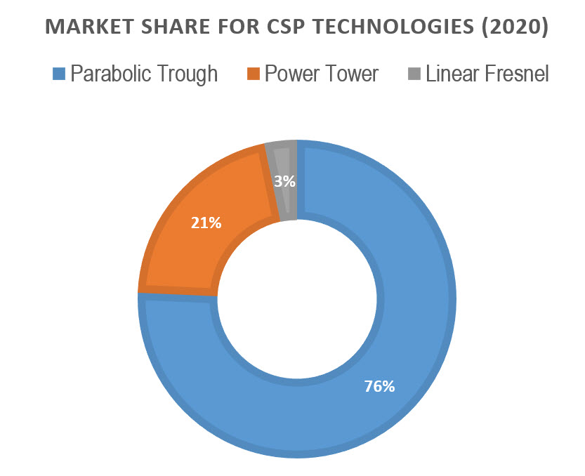
Further, in this lesson, you will learn about different configurations of CSP plants, which differ in design of optical systems (reflectors and light collectors), position of the receiver, and heat transfer networks. These various technologies have their pros and cons and are applied based on the target application, location, and other factors.
7.2. Parabolic Trough CSP Technology
7.2. Parabolic Trough CSP Technology
As was noted earlier in this course, parabolic trough technology is the most widespread among utility-scale solar thermal plants (Figure 7.1). The potential of this type of solar concentration is very high and can provide output fluid temperatures in the range 400-500°C. Parabolic trough is the linear-focus collector, which consists of a cylindrically curved parabolic mirror, which reflects the sunlight onto a tubular receiver positioned in the focus line of the parabola. The tubular receiver contains the fluid that absorbs heat and transfers it via circulation to the boiler or another device to produce steam.
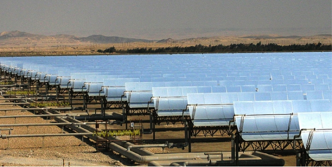
We covered the basics of light concentration by parabolic reflectors in Lesson 2. Now, we go on to look at all different aspects of the parabolic trough technology, including materials, operation parameters, system design, field layout, energy storage associated with this kind of plant. Please refer to the following reading material:
Reading Assignment
Book chapter: Zarza Moya, E. Parabolic-Trough Concentrating Solar Power (CSP) Systems, Chapter 7 in Concentrating Solar Power Technology. Principles, Developments, and Applications., Lovegrove K., and Stein W., Eds., Woodhead Publishing, 2012. pp. 197-237. (See E-Reserves via the Library Resources tab.)
Based on the above reading, please go through the following self-check questions.
Check Your Understanding - Essay Question
Question 1. How do the small and large parabolic trough collectors (PTC) compare in size? Put in typical numbers for trough width:
Small collector:
Large collector:
Question 2. What is the purpose of the glass pipe in the design of a tubular receiver?
Question 3. What are three main blocks of a typical parabolic-trough solar thermal plant?
Question 4. What are the maximum theoretical and actual concentration ratios determined for the parabolic trough collectors (approximately)?
Theoretical:
Actual:
Question 5. What four factors are responsible for optical losses of the parabolic trough collector?
7.3. Central Tower CSP Technology
7.3. Central Tower CSP Technology
Unlike linear concentrating systems (troughs), which reflect light onto a focal line, the central receiver systems send concentrated light onto a remote central receiver. A typical example of such a system is a solar power tower system, which consists of multiple tracking mirrors (heliostats) positioned in the field around a main external receiver installed on a tower (Figure 7.2). Such systems are capable of reaching of much higher levels of concentration than linear systems. Concentrated radiation is further used as heat to produce steam and convert it to electricity (like in a regular power plant), or the generated thermal energy can be stored in a molten salt storage.
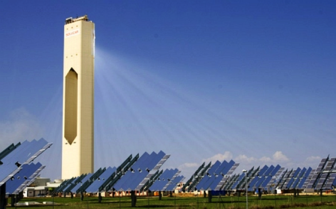
Please proceed further to the following chapter reading, which covers some basic configurations and design of the central receiver CSP technology, approaches used to convert and store energy, specifications of the heliostats and receivers utilized in some known facilities of this type.
Reading Assignment
Book chapter: Vant-Hull, L.L., Central Tower Concentrating Solar Power (SCP), Chapter 8 in Concentrating Solar Power Technology. Principles, Developments, and Applications., Lovegrove K., and Stein W., Eds., Woodhead Publishing, 2012. pp. 240-281. (See E-Reserves via the Library Resources tab.)
It is clear that central receiver CSP systems are typically large-scale plants that are usually built to power a steam cycle. The central position of the receiver offers a universal advantage to collect all energy at one location and save on transport networks. At the same time, the fixed position of such a central receiver results in limitation of light collection: heliostats are always oriented at an angle to the direct beam, so the amount of energy collected is less compared to parabolic concentrators. Therefore, to reach the necessary efficiencies of light concentration, the size of the collecting field is increased, which brings into considerations such issues as land use, higher environmental impacts, and higher capital costs. Significant potential for developing large-scale central receiver solar plants is hence attributed to deserts and flat arid areas, which have plenty of sunshine and lower land value with respect to other applications and industries.
Check Your Understanding - Essay Question
Question 6. Can you name and explain the three main configurations of the central receiver CSP systems?
(1)
(2)
(3)
Question 7. What are the main disadvantages of the external cylinder receiver system compared to cavity receiver system?
Question 8. What are the main advantages of the external cylinder receiver system compared to cavity receiver system?
Question 9. What are the insolation requirements for a good central receiver CSP facility?
Peak direct beam insolation:
Annual bean insolation:
Question 10. What are most typical options for heat transfer fluids at the central receiver CSP plants?
7.4. Parabolic Dish CSP Technology
7.4. Parabolic Dish CSP Technology
Parabolic dish geometry concentrates light in a single focal point, i.e., all sun rays that are parallel to the axis of the parabola are directed towards the central receiver. This allows this type of collector to achieve the highest concentration ratios among all other type of solar collectors. The dish concentrator must be oriented towards the sun. Usually, losses in this technology are associated with the imperfections of dish alignment and non-ideality of reflection. The engine that converts the concentrated solar energy into electricity is placed at the focal point. This technology can be used for both large-scale power plants (with many dishes grouped in arrays) and autonomous small-scale power generation systems that would provide power to off-grid remote facilities. Example of such a system is shown in Figure 7.3.
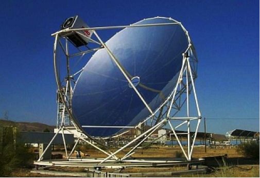
Go to the following chapter reading to learn the fundamentals of the parabolic dish CSP technology:
Reading Assignment
Book chapter: Schiel, W., and Keck, T., Parabolic Dish Concentrating Solar Power (CSP) Systems, Chapter 9 in Concentrating Solar Power Technology. Principles, Developments, and Applications., Lovegrove K., and Stein W., Eds., Woodhead Publishing, 2012. pp. 284-321. (See E-Reserves via the Library Resources tab.)
As we can see from this reading, the parabolic dish is a very efficient and flexible technology, which comes in various designs and is suitable for various applications. There are many cases (some described in the history section) of applying this technology in remote locations to provide self-sustained power for water heating, water pumping, and alternative power. One of the features of the dish Stirling systems is their low "inertia" - they start producing power very quickly as soon as direct beam radiation hits the reflector, but, at the same time, they are very sensitive to variations in solar intensity and results in sharp variation in power output and frequent interruptions if the meteorological conditions are not perfect. Because of the high intermittence, energy storage applications which would buffer the power output, would be desirable, but at the moment are not well developed.
Note:
Please take a note of pros and cons of this technology. In the end of this lesson, you will be asked to make a comparison of a few technologies by common metrics. You can revisit some quick facts of the dish Stirling technology by answering the following self-check questions
Check Your Understanding Questions 11-15 (Multiple Choice)
7.5. Thermal - electric power conversion
7.5. Thermal - electric power conversion
To make usable energy from solar heat collection in CSP plants, thermodynamic power conversion cycles (heat engines) are used. The main idea is quite simple. The heat transfer fluid, which is directly heated in the solar receivers, delivers heat to the boiler, which generates steam. Further steam is used in the heat engine to generate mechanical work to run electric generator. This scheme is very much the same as at conventional fossil fuel power plants, except for the heat being created not through combustion but through concentration of solar radiation.
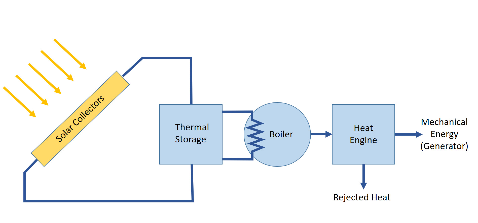
Note
The physics of thermodynamic cycles is something you might have learned in a typical thermo class (if you have ever taken one). If not, this topic may be somewhat challenging to grasp outside the general thermodynamics context. I should note, however, that the main goal of our activity in this lesson will be to understand the general principle and applicability of different power conversion cycles to solar systems, not learning thermodynamics in detail. So, while going through readings in this lesson, you can try to filter things down to the information that would be useful from the solar project development perspective.
In general, the thermodynamic power cycles can be categorized into gas cycles and vapor cycles. In gas cycles, the working fluid is only present in the gas phase throughout the entire cycle. In vapor cycles, the working fluid can be transformed from the vapor phase to the liquid phase in different parts of the cycle. Rankine cycle, commonly used in stationary steam power plants, is an example of a vapor cycle with water as a working fluid.
In the course of a thermodynamic power cycle, the working fluid goes through a series of temperature and pressure (T,P) parameters. Changes in temperature and pressure result from heating, condensing, pressurizing, and expanding the fluid medium. Expansion creates the physical force to perform mechanical work, which is the main purpose of the system. The efficiency of the cycle is typically higher when the difference between the lowest and highest temperatures is maximized. For example, Carnot efficiency is:
The maximum temperature is set by the heating source - for example, solar concentrator. The minimum temperature is set by the ambient conditions or cooling system - for example, air, river. The Carnot efficiency of 50% is considered good for a real system.
Note
One of the problems of this conversion system is that the efficiency of a solar collector decreases as its operating temperature rises (due to increased heat losses), while it is the opposite for the heat engine part of the system, which benefits from the higher maximum temperatures. So optimization of the system has to be done to find the best operating conditions.
Several thermodynamic cycles that may be considered in connection to solar thermal applications are:
- Rankine Cycle
- Brayton Cycle
- Stirling Cycle
- Kalina Cycle
One of the criteria to combine these cycles with the solar thermal plants is the compatibility of temperature. The concentrating technologies must be efficient enough to generate high temperatures for efficient power conversion in the thermodynamic cycle. So, depending on the technology and type of solar collectors, one or another cycle may be chosen.
Another important criterion to consider is the choice of the working fluid. For higher temperatures (600 oC), steam is the best choice. For lower temperature conversions (100-400 oC), organic fluids are more suitable (Batton, 2000). The desirable properties of the working fluid are:
- low cost
- non-corrosive nature
- thermal stability
- high cycle and turbine efficiency
Possible choices for the working fluids include:
- water
- refrigerants
- organics
- ammonia
- toluene (under development)
- mixtures of above
- fully fluorinated benzene ring fluids
Currently, Rankine cycles are most promising for handling the collector temperatures.
7.6. Rankine cycle
7.6. Rankine cycle
We are going to overview the principle of thermodynamic cycle operation using Rankine cycle example, since most of solar power cycles currently operating are Rankine cycles.
The Rankine cycle system consists of a pump, boiler, turbine, and condenser. The pump delivers liquid water to the boiler. The boiler heated by the solar heat converts water to superheated steam. This steam is used to run the turbine which powers the generator. Steam leaves the turbine and becomes cooled to liquid state in the condenser. Then the liquid is pressurized by the pump and goes back to the boiler. And the cycle continues. Schematically, this process is represented in Figure 10.1.
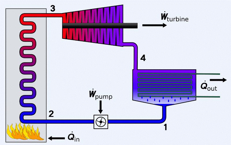
In an ideal Rankine cycle, all the units operate with the steady-state flow, and the kinetic and potential energy of the fluid are considered to be negligible compared to the temperature and pressure effects.
The work terms for each component of the cycle can be expressed as follows.
The work done by the pump to compress water (Wpump) can be represented as the change in enthalpy (H) of the water (fluid) before entering the pump and after leaving the pump:
In this case, we assume there is no heat exchange with the surroundings, so the energy is not lost (which is an ideal scenario). The process, which is not accompanied by any heat exchange with the environment, is termed "adiabatic." So, this step 1-2 is adiabatic compression.
The next process 2-3 takes place in the boiler. The energy balance in the boiler can be expressed as the change in enthalpy of the fluid from the "before" state (compressed liquid) to "after" state (superheated steam):
Where Qin is the heat used by the boiler. This heat is supplied to the boiler from the solar concentrator. There is no pressure change in the boiler, only heat transfer to the fluid; therefore, no mechanical work is done here.
The next process 3-4 is expansion of the steam in the turbine. The work done through that process is the useful work, which is the main purpose of the cycle:
Here, we again assume that there is no heat exchange with the surrounding, so all the fluid energy change is converted to work. Note that the enthalpy change is written as "before" minus "after" because the energy of the superheated compressed steam is higher than the expanded steam after it exits the turbine. So, this expression gives us the positive work value.
Lastly, the process 4-1 is steam cooling and condensation. The energy balance on the condenser will be:
At this stage, the extra heat is withdrawn from the system, and water returns to liquid state. This is important for the Rankine cycle from technological standpoint, since pumps employed in the system require liquid medium to work efficiently and may have problems with water-vapor mixtures.
The energy balance for the whole cycle is then can be expressed via the following equation:
The net work done by the system is Wturbine-Wpump. Therefore, the thermal efficiency of this cycle can be presented as follows:
The basic Rankine cycle is presented in terms of temperature and entropy change in Figure 10.2. The ideal state of this cycle is reflected in the vertical lines 1-2 and 3-4, when the fluid compressed and expanded. Those processes are shown to proceed isentropically, i.e., without entropy change. That rarely happens in real life. Some fluid friction losses and dissipation of some heat to the surrounding usually makes this system deviate from the ideality (as for example, shown by the dashed lines).
In a non-ideal cycle, fluid friction results in the lower pressure in the line. To compensate for this pressure drop, the water needs to be pumped to a higher pressure. Heat loss can happen when steam flows through the connecting pipes and the cycle components, which are not perfectly insulated. To maintain the same work output, more heat needs to be transferred to the steam in the boiler.
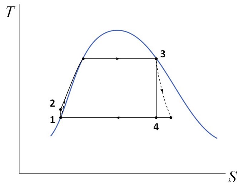
Varieties of the Rankine Cycle
There are several scenarios of employment of the Rankine steam cycle in power plants, including solar plants. Those scenarios intend to increase the overall efficiency of the system.
There are three ways to increase the efficiency of the basic Rankine cycle (Gramoll, 2015):
- Decreasing condenser pressure. This results in lower heat rejection temperature of the fluid in the condenser (pushing point 4 on the diagram in Fig. 10.2 downward), thus allowing the system to produce greater net work.
- Superheating steam to a higher temperature allows achieving higher temperature differential, thus increasing the amount of work done by the cycle.
- Increasing the boiler pressure results in higher average steam temperature in the boiler. This effect allows additional work to be done in phase 2-3 (Fig. 10.3c). However, there is some loss of useful work in phase 3-4 because of necessity to re-heat the steam. Reheating is used to mitigate higher moisture content of the high-pressure steam.
The above-described efficiency modifications are illustrated in Figure 10.3.
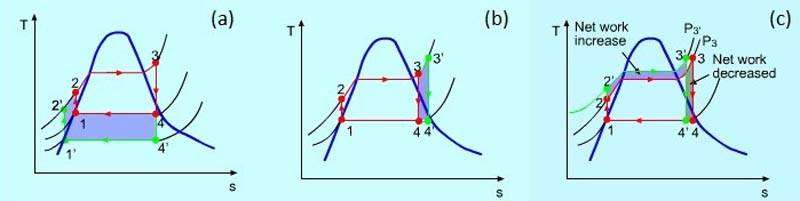
Another variety of Rankine cycle is the Regenerative Rankine. The idea behind the regenerative cycle is to increase the temperature of the feed water that is supplied to the boiler. Why is it desirable? Higher water temperature would allow some energy savings for steam generation. So, some of the steam that exits the turbine is used for pre-heating the feed water for the boiler. This process is called regeneration. Heat transfer can be achieved using a heat exchanger (regenerator). There are two types of feed water heaters: open and closed.
The open feed water heater is essentially a mixing chamber, where the steam extracted from turbine is combined with water from the pump. The fluid that exits the mixing chamber is saturated water. The closed feed water heater is a heat exchanger, inside which the steam condenses on the outside of the tube carrying the feed water. As a result, the feed water temperature is increased. The pressures of the steam and the feed water do not need to be matched since the flows are not mixing. Without heat regeneration, the feed water temperature would be much lower and would require more energy from the heat source for the boiler. Regeneration helps raise the overall efficiency of the system.
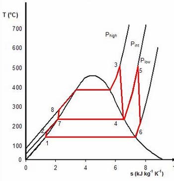
Reading Assignment
The following reading material contains more details on the Rankine cycle and other power conversion cycles that potentially (now or in the future) can be applied to utility-scale solar power systems.
Book chapter: Stine, W.B. and Harrigan, R.W., Power from the Sun, Chapter 12 Power Cycles for Electricity Generation [91], 2001
This reading contains some thermodynamic language that may be beyond the scope of this course, but stay cool. Your goal of studying this material will be quite practical - compare the Rankine, Brayton, and Stirling cycles and extract information on the following:
- Main principle of the each cycle: how steps of compression, heating, and expansion (work performing) are performed
- Temperature range: this will be important for matching a specific power-conversion cycle with a certain type of solar thermal system
- Working fluid
- Efficiency
- Compatibility with solar and examples of that if available.
Note: This material will be needed to answer questions in this Lesson quiz!
Summary and Activities
Summary and Activities
In this lesson, we looked at the types, design, and components of the Concentrating Solar Power (CSP) systems - parabolic trough, solar power tower, and parabolic dish. All of these types of CSP systems essentially differ in the way how they collect and concentrate light, and how the thermal energy is transferred. There is not as much difference in the final application (with some exceptions of course), as the output energy is primarily used to produce steam and run a turbine for electricity generation. The second half of this lesson reviewed the power converion cycles that accomplish that task. Based on this lesson, you should have a clear idea on the principle of operation of each of those types of systems and should be able to explain and compare the key specifications of CSP plants. Certainly, planning of a large-scale CSP plant is a complex task, which includes not only the technical principles of energy concentration and conversion. The major decisions are also made regarding the climate setting, solar resource, policy, and cost. Those considerations involved in strategic planning of CSP projects will be addressed further in Lesson 8.
The thermodynamic power conversion cycles used to convert heat into mechanical energy (and eventually electric power) are not novel technologies. Most of those cycles were technologically developed through 20th century and were widely applied in traditional fossil fuel fired plants. However, integration of those systems in solar CSP power plants may require some adjustments to match both system parameters. Rankine cycle has been most applicable to solar power plants to date as it operates in the lowest temperature range and therefore requires the lower concentration ratios. Stirling and Brayton cycles require higher temperature range and are suitable for higher concentration ratios, like those in central receiver systems. This lesson gives you a few examples of practical implementation of power conversion cycles in existing solar facilities.
| Type | Description/Instructions | Deadline |
|---|---|---|
| Readings | Complete all necessary reading assigned in this lesson. | -- |
| Reading Quiz |
|
Sunday night |
| Activity |
Comparative Table 1. Search and compile information on the key CSP technologies:
You can use the materials given in Lesson 7 and/or search other resources. 2. Identify several key metrics to compare those systems. These should include operational parameters (e.g. concentration ratios, efficiency, output), compatible power conversion cycles (e.g. Rankine, Brayton etc.), and cost metrics (e.g. LCOE etc.) 3. Create a summary table to classify the information you collected by those metrics. This will be the main outcome of your work. 4. Cite sources for the information included in your table. |
Wednesday night |
References
Batton, W., Organic Rankine Cycle Engines for Solar Power, Solar 2000, Madison WI. URL: http://organicrankine.com/orc_documents/theory/21036.pdf [101]
Gramoll, K., Multimedia Engineering Thermodynamics, Ch. 10 Rankine Cycle, eCourses, Accessed 2015. URL: http://www.ecourses.ou.edu/cgi-bin/ebook.cgi?doc=&topic=th&chap_sec=10.0 [102]
Duffie, J.A. and Beckman, W.A., Solar Engineering of Thermal Processes, Wiley 2013
Stine, W.B. and Harrigan, R.W., Power from the Sun [103], (online book), 2001.
Lesson 8: Concentrating Solar Power Strategies
Overview
Overview
Lesson 8 will cover a few important issues related to planning the large-scale CSP facilities. As we have already understood, performance of solar systems is very dependent on the locale, weather, and other physical conditions. Therefore, selection of a good site for a CSP project is a strategic step to take in order to ensure that the technology performs to its potential. So, criteria to consider in site selection are addressed in this lesson. Next, we will take a look at some factors in the social and economic spheres that pertinent to success of the solar projects. Finally, this lesson also touches upon the life cycle assessment of the CSP technology - LCA study examines a variety of metrics, which help to constrain the project with available resources and produced environmental impacts. In this lesson, you will be assigned to learn from a couple of published papers which present different methods of project assessment. Also, a lesson activity done in SAM software will give you some practical exercise with system parameters.
Learning Outcomes
By the end of this lesson, you should be able to:
- understand the prerequisites for location of a CSP plant;
- demonstrate the basics of the feasibility analysis for CSP systems;
- define the key metrics used in socio-economic and environmental assessment of the CSP projects;
- generate CSP system performance data in SAM software.
Readings
Report: Stoddard, L., Owens, B., Morse, F., and Kearney, D., New Mexico Concentrating Solar Plant Feasibility Study [104], Report to New Mexico Energy, Minerals and Natural Resources Department, 2005.
Journal article: Lechon, Y., de la Rua, C., and Saez, R., Life Cycle Environmental Impacts of Electricity Production by Solarthermal Power Plants in Spain [105], J. Solar Energy Eng., 130, (2008).
Journal article: Caldes, N., Varela, M., Santamaria, M., and Saez, R., Economic impact of solar thermal electricity deployment in Spain [106], Energy Policy 37, 1628-1636 (2009).
8.1. CSP site selection and feasibility analysis
8.1. CSP site selection and feasibility analysis
Solar energy systems rely on the natural solar resource, which is unevenly distributed over the planet. Clearly, some locations may be considered very favorable for harvesting sunlight, while others - much less favorable for a number of reasons. Choice of the CSP development site has therefore a strategic importance for the long-term feasibility of the project. Meteorological availability of sunlight is the first, but not the only, limitation to be considered when planning a CSP site development. One should also look at the physical geography of a potential site, available land area, available infrastructure, energy market, political and social situation. All these factors, being location-specific, can have a critical influence on the success of the CSP development in the area. In essence, the project development approach to CSP is no different from other project developments, such as those involving conventional fossil fuel power plants, photovoltaic solar, wind, etc. However, CSP has its own specific features that require special knowledge when site selection and feasibility study are performed.
Any site targeted for CSP should be carefully examined with respect to the key criteria. The most important of them are listed below:
- Direct normal irradiance (DNI). This is the amount of solar radiation received by a unit area that is perpendicular (i.e., normal) to the incoming sun rays. DNI converts to energy, which, in turn, converts to monetary return from the project. It is generally believed that DNI should be at least 2000 kWh/m2 per year to provide a viable energy yield [Lovegrove and Stein, 2012]; however, the threshold would depend on the local market, and should be assessed individually for each case. The accuracy of the DNI data is very important for estimating predicted energy output from the future plant. It is recommended to perform on-site DNI measurements for at least one year to characterize a complete seasonal cycle.
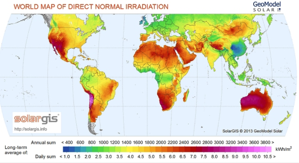 Figure 8.1. World map of DNI.Credit: SolarGIS © 2014 GeoModel Solar. Refer to the SolarGIS [107] website to get the DNI maps for specific locations.
 - Available land area and topography. These conditions are different for different CSP technologies. For example, parabolic trough setup tolerates up to 2o slope, while Fresnel reflector systems can tolerate up to 5o slope. Solar tower systems can accommodate more variegated topography as long as the slopes properly support the arrangement of the heliostats. Typically, utility scale CSP plants requires substantial area of open land (~ 2-5 km2) free from obstructions. Typical land use by CSP plants was estimated by NREL at ~40,000 m2/MW [NREL, 2013].
- Soil and subsoil structures. The land should allow some leveling works to be performed. This requires the analysis of soil and rock conditions. Some soft soils may be unstable and undermine the alignment of optics; so, it may need to be replaced. Rocky formations underneath may bring extra costs for leveling works.
- Weather profile. Long-term data analysis of meteorological and satellite data helps to create predictions for the cloudiness in the area over the system lifetime. Also, strong tendencies for rain, water run-off, or flooding may have effect on site topography. Strong winds may have a direct impact on power generation since they create vibrations and deformations on concentrators and thus affect sunbeam focusing precision. Some sites benefit from wind-breaking barriers and other mitigation measures. Dry bulb and wet bulb temperatures are assessed to define the achievable cold-end temperatures of the power plant. This has effect on the steam turbine efficiency.
- Local water resources. Water is needed for CSP plants first of all as the cooling agent for steam turbine condenser. Both subsurface and surface water can be used. However, the locations with highest DNI are typically arid areas (e.g., deserts), where water is scarce. Associated need for water use authorization may become an additional obstacle for site approval. Other water use includes service, mirror cleaning. Water-steam cycle requires demineralized water, which would require an additional on-site water treatment plant.
- Grid connections. The power produced must be delivered to customers, so the connection to the high voltage electricity line is necessary. CSP plants of 20 MW and above capacity usually use the lines in the range of 60-400 kV. The distance to the grid should be minimal to avoid additional investments for power transmission. If auxiliary routes for power transmission need to be constructed, authorization and environmental concerns should be addressed up front.
- Proximity of roads. Roads are needed at the stage of plant construction for transport of materials and equipment to the site. Further, at the operation stage, access roads become permanent structures.
The simultaneous analysis of the multiple factors make the site assessment a complex iterative process. The main successive phases of this process are illustrated below (Lovegrove and Stein, 2012):
1. Market Analysis
- Analysis of interest and suitability of CSP
- Identification of targeted markets
2. Regional Stud and Site Identification
- GIS data assessment: is DNI promising for this region?
- Infrastructure analysis for the main phases of the project
- Finding potential sites for the project
- Identification of CSP technologies and technical concept
3. Feasibility Analysis
- DNI assessment / measurement
- Identification of potential fatal flaws, risks
- Geotechnical and topographic site assessment
- Detailed economic analysis / financial modeling
- Socio-economic analysis
4. Project Qualification
- Expert assessment of solar resource and yield
- Environmental impact assessment
- Geotechnical and topographic survey
- Obtaining permits and authorizations
- Contract negotiations
- Obtaining equipment price quotes
5. Contract Closing
- Completion of legal steps
- Risk assessments
- Construction contract
- Equity and debt agreements
Each subsequent stage in the above scheme requires more specific information and additional expertise. This process of site characterization and selection is to some extent illustrated in the report by Stoddard et al. (2005) - the study that considered various alternatives for CSP plant development in New Mexico:
Reading Assignment
Report: Stoddard, L., Owens, B., Morse, F., and Kearney, D., New Mexico Concentrating Solar Plant Feasibility Study [104], Report to New Mexico Energy, Minerals and Natural Resources Department, 2005.
Please read Section 3.0 of the document. Especially pay attention to Table 3-1, which provides a comparative matrix for nine different sites with potential for CSP development.
Water considerations
The water use strategy at the CSP facility is one of the keystones of the project, as it would influence many other factors and choices and may become a go/no-go tipping point for the project. This is because water shortage is being identified as a severe environmental problem in many regions, and, therefore, is subject to strict environmental regulations. So, let us take a closer look at the water requirements in CSP systems and associated technological options.
The biggest consumption point of water in CSP is cooling for the steam turbine condenser. Cooling systems can utilize both salt and fresh water, which can be taken from both surface and subsurface reservoirs. Agreement on water withdrawal should be reached prior to the project start, and that should be part of the project feasibility analysis. There are wet-cooling and dry-cooling systems. The wet cooling usually implies using a cooling tower, and that is the most efficient technology for cooling as long as water is affordable and continuously available for plant operation.
If you are not familiar with those, watch the following video (3:16) to see how they work:
Video: How Cooling Towers WorkV (3:16)
Cooling towers are devices used to transfer heat or cool water for reuse.
The basic operation is fairly simple. Hot water is pumped in from an outside source and sprayed into the tower. The hot water flows over what is called the fill. This spreads the water over a larger surface to allow for more cooling. Cool air flows over the fill, which transfers more heat through evaporation. The heat exits the tower, and the now cooler water gathers in the basin. This cooler water is then pumped back into the system to be used again.
Cooling towers are just one part of the cooling system. In this lesson, we will cover the basic process of how a cooling tower works, define the components, and describe their purposes, and we'll also cover some common terminology that is used when discussing cooling towers.
Within a cooling tower, you will see the use of plastic or wooden slats. These are called fill, and are used to direct the flow. The purpose of this is to increase the area of contact between the hot water and the cooler air.
There are two types of heat loss that occur in this process, sensible heat loss and evaporation. Sensible heat is what can be felt or measured. Evaporation accounts for the majority of the heat transfer and is the most critical aspect of the entire process.
Many factors can affect the efficiency of the evaporation in a cooling tower. Things such as relative humidity, outside temperature, and wind velocity can affect the efficiency. Even the design of the tower, water contamination, and outside equipment will also play a part.
Cooling towers are classified by how airflow is produced. This allows them to be broken down into two categories, atmospheric and mechanical draft. These two will be covered in detail in a separate video, but for now here's a quick description.
To see the rest of this video and many more, please visit us at CTESkills.com.
However, cooling towers use up to 85-90% of all process water. When water is in short supply, dry-cooling systems can be an alternative. Dry-cooling systems use ~10 times less water than wet cooling systems do; even truck-based supply may suffice. However, from an economic point of view, dry cooling systems are less beneficial. In dry cooling systems, air is used as heat transfer medium, and air has much lower heat transfer coefficient than water. Furthermore, the cooling effect of evaporation, which is the core mechanism of cooling in cooling towers, is not available. This results in lower efficiency of the water-steam cycle. Another drawback of the dry-cooling systems is additional power consumption by fans blowing air for cooling. For the above reasons, the wet-cooled projects have an economic advantage over dry-cooled projects. The decision involving the trade-off of water versus energy is to be made individually in each particular case based on available resources. One of the compromise options for water use is hybrid cooling tower, which combines dry cooling and wet cooling. In this technology, water is sprayed on the condenser allowing for evaporative action, but the water consumption is significantly lower compared to conventional wet cooling method.
According to water use estimation by Andrew Eilbert (Worldwatch Institute), on the average, CSP plants use only 120 Gal of water per megawatt-hour of energy. For comparison, this number is lined up against typical values for other types of power plants in Table 8.1. [Eilbert, 2010]. Visit the WorldWatch website [109] for specific data on water use by different CSP plants in California.
| Type of power plant | Average lifecycle water use |
|---|---|
| CSP (with dry or wet cooling) | ~120 gal/MWh |
| Powder River Basin coal power plant | 523 - 1,084 gal/MWh |
| Conventional natural gas combined cycle power plant with wet cooling | 152 - 525 gal/MWh |
| Conventional nuclear power plant with wet cooling | 475 - 900 gal/MWh |
Other water uses in CSP plants include:
- process (water-steam cycle)
- service (cooling rotating equipment)
- washing (mirror cleaning)
The water involved in water-steam cycle needs to be relatively pure and often needs to be de-mineralized. Requirements for water purity is specified by the turbine manufacturers. These requirements impose an additional limitation on the water sources. If raw water contains significant amounts of ions and other chemicals, a special water treatment plant may need to be added to the facility. Much of this water is recycled, and its total volume is not substantial.
Please answer the following self-check questions before proceeding to the next section.
Check Your Understanding Questions 1 & 2 (Multiple Choice)
Check Your Understanding Question 3 (Essay)
What are the main types of site-related costs to consider in site selection?
Additional Resources for Section 8.1
8.2. Socio-economic aspects of CSP technology
8.2. Socio-economic aspects of CSP technology
CSP deployment has a number of positive collateral impacts on environment and social welfare, and those impacts are important to consider in the project feasibility analysis. Sometimes, when project evaluation is solely based on the energy prices, renewable energy technologies may not look competitive enough at the modern energy market. However, including externalities, such as greenhouse gas emission reduction effect, improved diversity, security of the energy supply, employment, etc., into the evaluation process can help to justify the value of a renewable energy project more fairly.
One of the prominent impacts of CSP in the socio-economic area is stimulation of the economy and creation of new jobs at the local level. This is largely due to relatively "low-tech" profile of this technology: the main components are mirrors, steel, concrete, and labor. These local impacts are realized through the increase in demand for goods and services and creation of jobs. These impacts can be classified as direct, indirect, and induced.
The direct effects imply the increased demand for good and services that are required to construct, operate, and maintain the CSP facility. The indirect effects involve the one the new investment has on new sales and material flows among other productive sectors of the economy. The induced effects are related to expansion of private expenditure (for example, from workers employed) in goods and services, such as food, health care, transportation, etc. [Lovegrove, Stein, 2012]. For proper accounting of all levels of external benefits, there should be a way to quantify them and to assign them a monetary value.
One of the analytical methods to quantify the externalities of energy projects is based on Input-Output (I-O) analysis. The I-O analysis is an economic theory that was developed by Wassily Leontieff, a Russian economist who received a Nobel Prize for it. This model describes the inter-industry relationships within an economy, connecting the outputs from one part of the economy to the inputs to another part of the economy. The data are typically expressed as monetary values and are organized as a matrix, with column entries representing inputs to an industrial sector, and rows representing outputs from that sector. [Input-Output Model from Wikipedia.org [111] ]. Essentially, this approach recognizes that spent investment becomes income to other industries, and thus stimulates their development.
To understand how this method can be applied to CSP projects, we refer to the following publication, which analyzes the socio-economic impacts of parabolic-trough and solar-tower plants in Spain. The authors come up with impressive numbers for increase in demand and employment impacts, demonstrating the remarkable potential of CSP for benefiting local economy.
Reading Assignment
Journal article: Caldes, N., Varela, M., Santamaria, M., and Saez, R., Economic impact of solar thermal electricity deployment in Spain, Energy Policy 37, 1628-1636 (2009).
This article is available online through the PSU library system. See copy of the article in Canvas Module 8.
This article nicely demonstrates the quantified benefits from solar thermal energy projects, which are rarely taken into account in feasibility analysis. The type of analysis presented there is a convenient tool to determine whether the government subsidies provided to defray the cost of the renewable technology are justified in terms of social welfare.
Some main points in the above-mentioned study are included in the self-check questions below.
Check Your Understanding Questions 4-6 (Multiple Choice)
8.3. Environmental assessment of CSP Technology
8.3. Environmental assessment of CSP Technology
As a technology based on the renewable solar resource, the CSP has a great potential to reduce greenhouse gas (GHG) emissions. Emissions typically associated with conventional electricity production result from coal or natural gas burning and have been a severe factor in global pollution in climate change. Hence, installation of CSP offsets generation from fossil fuel plants. It does not mean, however, that CSP technology is emission free: while operational emissions are negligible compared to fossil-fuel power plants, lifecycle emissions may be still significant. To estimate the GHG emission level and the magnitude of the emission reduction benefit, one can employ Life Cycle Assessment (LCA) - a comprehensive methodology dealing with inventory of all processes and materials involved in a technology.
Life Cycle Assessment (LCA) methodology
Life Cycle Assessment (LCA) is a “cradle-to-grave” approach for assessing products, processes, industrial systems, and the like. “Cradle-to-grave” begins with the gathering of raw materials from the earth to create the product and ends at the point when all materials are returned to the earth. LCA evaluates all stages of a product's life from the perspective that they are interdependent, meaning that one operation leads to the next. LCA enables the estimation of the cumulative environmental impacts resulting from all stages in the product life cycle, and, as a result, allows selecting a path or process that is more environmentally benign.
LCA helps decision-makers select the product, process, or technology that results in the least impact to the environment. This information can be used with other factors, such as cost and performance data, to find optimal solutions. LCA identifies the transfer of environmental impacts from one media to another (for instance: a new process may lower air emissions, but creates more wastewater, etc.) and between different lifecycle stages. The diagram below illustrates the main lifecycle stages to be considered in LCA:
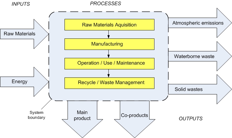
Figure 8.2. The main flows and stages considered in lifecycle assessment.
The diagram above lists the main stages of product lifecycle: (1) raw material acquisition, (2) manufacturing / construction, (3) operation or use, and (4) recycling or waste disposal (decommission stage). Each of these stages has inputs of materials and energy and outputs of atmospheric emissions, waterborne wastes and solid wastes. Each stage creates the main useful input to the next stage, and usually the operational stage of the lifecycle is where the main product of the technology is produced. Any co-products (desirable or undesirable) are also identified and taken into account in the analysis. The LCA based on this scheme is a complex process (even for small systems), which requires large amount of data and interdisciplinary expertise for proper assessment. A typical LCA project plan includes the following main steps:
- Goal definition and scope: Identify a product / process / technology; establish context and system boundaries.
- Inventory analysis: Identify and quantify energy, water, and materials as inputs as well as environmental releases as outputs.
- Impact assessment: Assess the potential human and ecological effects, quantify metrics.
- Data interpretation: Compare data from Inventory Analysis and Impact Assessment stages to select or recommend a preferred product, process, or technology.
LCA Limitations:
- LCA thoroughness and accuracy will depend on the availability of data; gathering of data can be problematic; hence, a clear understanding of the uncertainty and assumptions is important.
- Classic LCA will not determine which product, process, or technology is the most cost-effective or top-performing; therefore, LCA needs to be combined with cost analysis, technical evaluation, and social metrics for comprehensive sustainability analysis.
- Unlike traditional risk assessment, LCA does not necessarily attempt to quantify any specific actual impacts. While seeking to establish a linkage between a system and potential impacts, LCA models are suitable for relative comparisons, but may be not sufficient for absolute predictions of risks.
- The standardized procedure for the LCA recommended for product and technology assessment in the U.S. is documented in the EPA guidelines referenced below.
Life Cycle Assessment: Principles and Practice [112], EPA/600/R-06/060, 2006.
LCA Methodology Applied to CSP Plants
When the LCA analysis is applied to a CSP plant, a number of impact metrics need to be identified. One of them, as mentioned above, is greenhouse gas emissions, but there are also other impacts that involve environmental harm. Other typically assessed impacts are acidification and eutrophication potential. Acidification is referred to as increase in acidity of natural waters and soils. It may cause loss of aquatic life, forests, and other plants in the area and increase ecotoxicity. Eutrophication is related to nutrient enriching in aquatic and terrestrial environments. It can cause harm to ecological system through a chain of feedbacks, change in dissolved oxygen contents.
With respect to above metrics, CSP offers significant benefits, according to various studies reviewed in Lovegrove and Stein (2012). Values of GHG emissions by CSP plant (in case of solar only operation - no hybrid systems with natural gas backup) are estimated in the range from 11 to 90 g CO2 equivalent per kWh of electric energy generated. For central tower plants, the emissions are on the lower side, and for the parabolic trough plants, the emissions are on the higher side of that range; but, in either case, these numbers are well below the values typical for other electricity generation facilities (Table 8.2).
| Technology | GHG emissions g CO2 equiv/kWh |
|---|---|
| CSP (solar thermal) | 11-90 |
| Solar photovoltaic (PV) | 57-109 |
| Nuclear power | 14 |
| Heavy oil condensing | 726 |
| Light oil gas turbine | 436 |
| Coal/lignite | 690-820 |
| Natural gas combined cycle | 391 |
The CSP emissions have been shown to increase by 650 g CO2 equiv./kWh if a fossil-fuel back-up is used and by 60 g CO2 equiv./kWh if heat storage is used. The different studies indicate that CSP's GHG emissions are mainly associated with steel and concrete used in solar field and tower, and salts used in storage systems. The use of synthetic salts instead of naturally mined salts for storage system results in an increase in GHG emissions by ~13 g CO2 equiv/kWh. Also, non-renewable electricity and materials may be used at the manufacturing stage of the project and in transportation to the site. It is known that the use of dry-cooling system instead of wet-cooling system increases GHG emissions by ~2 g CO2 equiv/kWh.
Acidification impact of CSP reported in the range 70-100 mg SO2 equiv/kWh. In case of hybrid plant (solar + fossil fuel backup), this number is substantially higher - 590-612 mg SO2 equiv/kWh. In case of eutrophication, the impact range is 6-10 mg PO4/kWh for solar only mode and ~50 PO4/kWh for hybrid mode.
It is important to note that these impacts take place during the operational phase only because the plant consumes power from the grid rather than power being produced on site.
A published study by Lechon and co-authors (2008), referenced below, describes the LCA analysis for CSP systems in more detail. The first two sections of the article define the method and scope of LCA, so you can just briefly look through those. It is more important to look at the data tables that contain specifications of the assessed facilities and various metrics. Usually, LCA studies collect considerable amounts of data, and our goal here is to learn to read and to interpret that information.
Reading Assignment
Journal article: Lechon, Y., de la Rua, C., and Saez, R., Life Cycle Environmental Impacts of Electricity Production by Solar thermal Power Plants in Spain, J. Solar Energy Eng., 130, (2008).
This article is available through the PSU library system. See a copy of this article in Module 8 in Canvas.
As you can understand from the above article, the energy consumption at different stages of the system lifecycle is still the main source of the environmental impact. The numbers characterizing two different CSP facilities in terms of energy consumed and energy generated are listed in Table 3, which is the basis for finding the lifecycle emissions. Also, pay attention to Table 6, where the emissions are itemized by system component. This itemization can be helpful in finding engineering solutions to further decrease the environmental impact of the technology. Note that the plants assessed in this study are hybrid (solar thermal + natural gas 15%), and this is the reason for higher overall GHG emissions calculated for this case compared to solar-only values given in Table 8.2 above.
Check Your Understanding Question 7 (Multiple Choice)
Check Your Understanding Question 8 (Essay)
What sources of GHG emissions can you assume at the construction phase of the CSP plant?
Check Your Understanding Question 9 (Multiple Choice)
8.4. Optimization of CSP Systems
8.4. Optimization of CSP Systems
The biggest challenge in prediction of the CSP performance coming from a projected solar thermal plant is the unsteady nature of the solar resource. Models involve weather and insolation data which bring in uncertainties in the final power output. So, it is not sufficient to calculate the annual energy yield simply by expected load hours, as it is usually done for conventional fossil fuel power stations.
The energy flow within a CSP plant follows a complex chain of transformations, each provided by a certain technology block. This step-wise energy flow can be represented by the following diagram:
Each step in the power conversion chain is performed by technological units, each characterized by a number of parameters, which can be optimized depending on the scale of the facility, external conditions, available resources, and other preferences. Simultaneous optimization of those parameters and computation of the power output can be done by System Advisor Model (SAM) software, distributed by the National Renewable Energy Laboratory (NREL). SAM currently is one of the widely used and most developed tools for solar plant modeling, which incorporates both energetic and economic parameters. SAM has a user-friendly graphic interface, which allows the operator to see diverse technical performance information in table and graphs.
In SAM, the setting for each of the above mentioned technological units can be predefined and controlled separately, which creates opportunities for simulating different solar systems at different locations.
If you are not yet familiar with how the SAM software works, please refer to the following video (35:08), which explains the basic things about the program interface.
Video: SAM Intro Webinar 1 of 5: User Interface Overview (35:08)
PRESENTER: As most of you know, SAM is a free computer program that you can download from NREL's website.
And basically, what the model does is it calculates a renewable energy system's hourly energy output over a single year. So it simulates the performance of a power system over a year and then calculates the cost of energy of that project over the life of the project.
So conceptually, the model combines a performance model with a financial model. Here's a diagram of the structure of the program. There are basically three conceptual parts to the software. There are the input pages, which we'll see in a moment. And then, there are the model results. And then, there's a simulation engine that makes calculations based on the input variables and reports the results.
There are some more advanced features-- including Excel Data Exchange and SamUL scripting, and some advanced simulation control options-- that we'll be covering in tomorrow's session.
So this next slide sort of shows a little bit more the conceptual model to help you picture what's going on with SAM. The simulation engine is an hourly model, as I mentioned before. It's based on TRNSYS, which is a simulation software developed at the University of Wisconsin.
The simulation engine does an hour-by-hour simulation of the power system. So in order to do hour-by-hour calculations, it requires hourly weather data, which you provide as input to the model, so that you've got a weather file with 8,760 hourly data points for the solar radiation, temperature, wind speed, and other weather factors that affect system performance.
And then, you also have the system description, which tells the simulation engine what size of system you're modeling and what complements your system is made of.
So the two green blocks are inputs, and the red circle represents a calculation process. And then, the blue rectangles represent outputs. So the simulation engine generates a set of hourly outputs, a set of hourly values representing the electric output of the system-- so kilowatt-hours for each hour of the year. And that's the basic output of the simulation engine.
It also outputs some intermediate variables. So if you're interested in looking in more detail at how the system is operating, you can see for example the energy output at different points of the system, perhaps coming out of the solar array for a PV system, or coming out of a solar field for concentrating solar power system. But the primary output of the simulation engine is the electric kilowatt-hours for each hour of the year.
Then, SAM adds up those hourly values to calculate the total annual output of the system. So that's one number that is then passed to the financial model. And the financial model calculates the cost of energy of producing electricity with your system, and that runs over some long period, a number of years. So it uses the annual output of the performance model for year one, and then calculates the cost of operating the system for each year over a 20- or 30-year analysis period.
OK, so next I'd like to jump right into SAM. This is what you see when you first open SAM, the welcome page. And it provides you with three different options for getting started using the model. You can either start with a sample file-- so here's a list of the sample files. So sample files are files that we've prepared that have a complete set of inputs and results or a range of different systems and different technologies that SAM can model.
You can also start with a new file or new project. And to do that, you just type the name of your project under Create a New Project, and then click Create. And then, there's a list of recent files. These are files that I've worked with over the last few weeks.
These three options are also available under the File menu. So File, you could start with a new project, open a sample file, or look through a list of recent files.
These other options-- open a GIF file is for anyone who's used version three of SAM, which is a legacy version that uses a different file format. So if you have files that you created using SAM version three, you can save them as a GIF file and open them in the current version of SAM.
OK, so I'll just start by opening a sample file. And I'll start with a sample PV system to show you around the user interface. A SAM file or SAM project-- I'll use those two terms interchangeably-- consists of one or more cases. And a case in SAM is sort of analogous to a worksheet in Excel. So an Excel workbook can have one worksheet or it can have several worksheets. In Excel, each worksheet is accessible by a tab, which are along the bottom of the page in Excel. But in SAM they're along the top.
Each case in SAM is a complete set of inputs and results. So they're intended to allow you to do comparisons of different analyses within a single file. So by switching between cases in the file, you can compare different analyses. So you might set up different cases to compare different financial scenarios, or you might set up different cases to compare different technologies, for example.
So in this PV sample file, we have a case for a residential PV system, another for a commercial system, and another for a utility system. And as I click the tabs, I can see the results for the different cases.
Along the left side of the window here we have the navigation menu, and each of the items in this menu is actually a button that you can click. And by clicking each button, you display the input page. So for example, the climate page shows the input page where you specify climate file for your analysis. Financing-- there's finance inputs. Human Incentives-- those are the incentives inputs.
At the bottom under the navigation menu here are buttons that allow you to control simulations, run simulations, and also to display the results page. So this graph button with the bar graph button on it here displays the results page. And this is where you see graphs and tables of the results after you've run simulations.
One thing you'll notice about SAM, whether you start a sample file or a new file, is that the values on all the input pages are already populated. The variables are all populated with values. SAM has a large number of input variables, and so in order to help you get started, we've just chosen representative values for all of the input variables.
It's up to you as the modeler, once you start actually using SAM, to take ownership of the input variables and make sure that they all make sense for your analysis. These are values that we on the development team have chosen that are fairly representative of projects, generally in the US. But of course, the values that you choose for your analyses are going to be very project-specific and depend on the location of the project and also what type of project.
So be aware that these input various variables, the input values, are representative. They aren't officially sanctioned values by either NREL or DOE.
So the process for using SAM is to go through each of these input pages and either choose values for your project or change them. So some variables you choose values from a dropdown list, and other variables are fields that allow you to type values. And once you've specified values for all of the input variables, then you run the simulation by clicking the green arrow button down here, which is the Run button.
The status bar up here in the sort of top-middle of the page tells you the status of the simulations when they run. And then, once simulations are finished running, SAM displays the results page where you can explore the results. For more advanced analyses, you can use the Configure Simulations button here to access advanced simulation options. And these, again, are ones that we'll be discussing tomorrow.
So the basic process is specify your inputs, run simulations, and review results. And if you want, optionally, you can configure more advanced analyses.
So the results page-- again, to display the results page, I'm clicking this button with the graphs on it. The results page is divided into a couple of sections. Under the navigation menu is the metrics table, which displays kind of general metrics of your project.
And I'll be going through these in a little bit more detail later on in the session, but I just wanted to point out the metrics table here and two of the more important metrics, which are annual energy-- this is the total electric generation for this system over one year. So it's the electric output of the system, in this case in year one of the analysis period. And then, the levelized cost of energy, which is one of the primary outputs of SAM. So in this case, we've modeled a system with a levelized cost of energy, or LCOE, of about $0.155 cents per kilowatt-hour.
Over on the right-hand side of the screen are where you see a bunch of graphs. SAM displays a set of default graphs, which we see here. You can also create your own custom graphs. And in this case, by default, we see four graphs. But you can change the number of graphs that appear in the results page by clicking the little thumbnail images of graphs at the bottom of the window.
So as I click buttons, I see different graphs. If I want to display two graphs, I hold down the Control key, and then, I can display two graphs, three graphs, or four graphs. So you can display up to four graphs on the results page.
The buttons along the top center of the window here control what you see on the results page. So right now we're in the View Graphs and Charts mode. I can also view the base case cash flow table by clicking Base Case Cash Flow.
So these are the results of the financial model. And each column represents a year. So Year 0, Year 1, Year 2, and so on. In this case, we have a 30-year project, so there's 30 years of data in the cash flow table.
And then, each row in the table shows detail in the cash flow. The after-tax cash flow row is the key output of the financial model, and it's down towards the bottom of the cash flow table.
This cash flow table is not an Excel spreadsheet. It sort of looks like one. And you can click the Send To Excel button here to export the cash flow table to Excel.
But when you do that, this Excel spreadsheet doesn't have any calculations. SAM just dumps the cash flow values into Excel so that you can see them and manipulate them if you want to use them in your own external model in Excel or do some of your own graphing outside of SAM. So be aware that the cash flow table is just a table of values. It's not connected to Excel on how to equate formulas.
You can also copy the data from this cash flow to the clipboard and paste it into Excel or any other program, or you can save the table as a comma-separated text file.
For those of you running SAM on a Mac, the Mac version of SAM can't control Excel. So the Send to Excel option is disabled for Mac versions, but you can always use the Save As CSV option to save your data for use in Excel on a Mac.
The Tabular Data Browser is a table-building tool that allows you to sort of build tables of all of the outputs in SAM, or many of the outputs in SAM. So for example, the metrics list here is a list of all of the metrics that are available in SAM. And by checking boxes here, I can build a table of metrics. And when you clear the checkbox, SAM removes the value from the table. And once you build a table, then you can send it to Excel or save it as CSV text to use in reports or other programs.
You can also export monthly data. So the monthly data-- these are averages of the hourly data by month. And then, you can also look at annual averages. So this is for each of the 30 years in the analysis period. These are the monthly averages, so months 1 through 12. I'm simultaneously showing monthly data and annual data on the table, which is why I have 1 column of 30 values and another column of 12 values.
I'll clear all of those and show the hourly data. So if you want to dig into the details of the simulation results, you can display the hourly data. And let's look at the derated DC outputs. So this is the net output of the PV system for each of the 8,760 hours in a year. So that's the main output of the simulation engine.
But I can also look at intermediate values. Here's the total incident radiation. This is the energy incident upon the PV array. And then, I can look at the derated DC output. So this is the DC output of the array. Sorry, I misspoke earlier. The main output is the derated AC output.
So here we can see the progression from energy incident on the array, energy output of the array, and then, energy output of the inverter or the entire system. So you can build this table, and then, you can export it to Excel to examine in more detail.
There's also an option for looking at results that you can access either using the Export and View Data button here or through the Results menu. This Export button shows these options are all equivalent to the options that are available on the results menu. So you can use either method to access these results.
So here, Graph Data option just exports all the data from the graphs to the clipboard or to Excel. That's sort of equivalent to this Copy Graph Data button on the results page when you're in View Graphs and Charts mode.
You can also export the cash flow table via the Results menu. That's equivalent to choosing one of these buttons when you're viewing the page in cash flow mode.
And then, there's this case summary. So this is an Excel workbook that has a bunch of worksheets in it with all of the data. So here's the cash flow table in Excel. Here's the metrics summary table in Excel, the data from the graphs that we were viewing in SAM when we created this summary spreadsheet, a summary of inputs, hourly data, the monthly averages, and annual averages.
So the summary spreadsheet some people find to be a useful way to look at the results. Again, you get to that from Results, Case Summary, or by clicking the Results button here and choosing Case Summary and then clicking Send to Excel.
Another option for viewing results is to use DView, by clicking either the View Hourly Time Series button in the export data window or on the Results menu choosing View Hourly Time Series. And this opens a separate program called DView that displays graphs of the hourly data.
And it's a pretty nifty tool. It's kind of hard to interpret tables of large numbers of values, like a table of 8,760 values. So these graphs kind of give you a snapshot of the data.
One of the more powerful graphs in DView is called a DMap. So once you open DView, you have options for viewing the 8,760 data in various formats. One is as the line graph. This is looking at the hourly data itself, and I can look at the derated AC power, the derated DC power. I can show a second graph by using the two columns of check boxes here. So I can look at cell temperature and inverter efficiency.
On the top graph, I can zoom in and zoom out. I can look at the entire year. The daily tab shows daily averages of the data. And again, I can use the checkboxes to choose what data I display. There's monthly averages, daily profiles by month, the DMap, which shows a snapshot of the entire year.
If we look at the AC power out, we have months on the x-axis and hours on the y-axis. So you can sort of see the daily shape for the entire year, and also the seasonal variation over the year. And then, there's other statistical summaries of the data.
And you can export this data either as an image, if you want to copy pictures of the graph to include in your reports or presentations. You can also export the data itself. So if you click Export Data here, it'll just export the data that's visible in the graph to a text file, which you can then manipulate.
So that's DView. And again, DView is a separate little program that SAM calls to display the hourly data. SAM automatically includes a copy of DView when you install it, so you don't need to install any separate software. But DView is handy if you have other hourly data on your computer that you want to look at. You can use the File Open command here to look at other hourly data.
So that's a quick summary of viewing results in SAM. A couple of other things I want to point out about the user interface before I show you an example. One is this Notes feature. You'll see at the top right corner of the page a little sticky icon that look like a sticky note. If you click that icon and type some text, SAM will store this bit of text with the climate page.
So it shows a little sticky note icon on the Climate button to indicate that there's a note for the climate page. And then, when you click on the climate page, then, the note appears. So this is useful if you're sharing files with colleagues. You can make notes to each other, or you can make notes to yourself to remember changes that you made or to store values temporarily, and so on.
You can have notes. These are tax credit incentive notes that only appear when the tax credit incentives page is showing. You can store notes with the results page.
Another feature is the Help System, which is a useful resource when you're learning to use the model. There are a few ways to access Help. One is on the Help menu. If you click one of these options, you can display the Help System.
This is a browser-based help system. There's also a PDF version of the help system. So this is the same information that's in Help, but as a PDF file. If you prefer to use that, you can print pages from the PDF file. You can also use the search feature in your PDF reader to find information.
When you're on a page in SAM, you can press the F1 key to open the help topic for that page. So we're on the payment incentives page, and I pressed F1. And that opened the payment incentives help topic. I could also click the Help button here, this little round circle with a question mark in it, to open the help topic for the payments and incentives page.
The way the help pages are set up, they open just showing the headings to kind of help you find information. So if you're looking for information about input variables on the payment incentives page, then you can expand the input variable reference heading to see a list of all the input variables and descriptions. And you can expand and collapse the headings using the plus-minus button at the top of each topic.
And then, these buttons over on the top right-- you can open your email browser already addressed to user support if you have questions. This is a link to the Google Group page for SAM. And then, this is a link to the SAM website.
OK, I'm going to take a moment to pause and take a quick look at questions here.
So there's a question about the color of the input fields. You'll notice that some of the input variables have blue type, and others have black type. So the ones with black type are values that you can edit, and the ones with blue type are ones that you cannot edit. So SAM calculates the values in blue.
Some of these questions we're going to address later, so I won't answer now.
I think I answered this question about hourly granularity. You can look at the results and the weather data, both as hourly data. So you can compare the weather data and the results using the Tabular Data browser on the results page. So here we see the incident total radiation. That's the input from the weather data. And then, here's the simulation output at hourly resolution.
The climate page also allows you to see the climate data. If you click View Hourly Data here, that opens DView so you can see the data in the weather file, in case you're interested in exploring the weather data. So you can look at the wind speed data and so on.
Here's a question about currency units. There's no facility in SAM to change units. You're kind of stuck with the units that are provided in SAM. If you're very careful, you could change values. If you wanted to do your financial and cost modeling using Euros or some other currency, you could change all these values to your currency.
But I would recommend converting everything to dollars because it'd be easy to miss a value somewhere and some of the internal calculations may be based on dollars. So in general, I would recommend doing your modeling in SAM in dollars. And then, as far as other units-- watts and so on-- you're stuck with the units there. We don't have a conversion facility in SAM.
And then, before I continue, I'll just repeat-- I see a few questions about the logistics. So we're going to try to post a recording of the session on the SAM website, and I will post a PowerPoint presentation that has the talking points that I'm speaking from that'll serve as an outline of the session.
As an activity in this lesson, you will use a few examples from SAM to explore the differences between different cases of CSP installations.
8.5. Thermal Energy Storage
8.5. Thermal Energy Storage
Different types of fluids are commonly used for storing thermal energy from concentrating solar power (CSP) facilities. CSP plants typically use two types of fluids: (1) heat-transfer fluid to transfer the thermal energy from the solar collectors through the pipes to the steam generator or storage, and (2) storage media fluid to store the thermal energy for a certain period of time before it is used on demand.
These are some available heat transfer and storage fluids currently used:
- Water
- Water-Glycol mixtures (for low temperature only)
- Mineral oils
- Synthetic thermal fluids
- Molten inorganic salts
- Molten metals
Water is the most available and cheapest fluid to use, but the problem with water is that it has very limited temperature range when it is liquid. Keeping water in liquid state above 100 oC requires high pressure, which adds significantly to system complexity and cost. Oils and other synthetic liquids are commonly used in CSP plants, as they have a much wider working temperature range. Molten salts are probably the most common storage medium (Wu et al., 2001), but are not the best heat transfer medium, because salt tends to solidify in tubes at lower temperatures, blocking transport. Additional heating will need to be provided in that case to start up the plant. There are developments for novel fluids that can be used for both heat transfer and storage at the same time (Moens and Blake, 2004). Some commonly used fluids and their working temperature ranges are shown in the diagram in Figure 9.1.
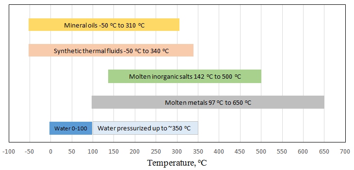
Molten salt storage is employed at many existing solar thermal plants, so we are going to look at it in some more detail. As was mentioned above, salt "freezing" (i.e., transforming from a molten state to solid state) can present some problems, because the salt is supposed to circulate through the tubes to deliver thermal energy to the steam generator or another application. So, to achieve the lowest possible "freezing" temperature, a eutectic mixture of salts is used.
What is eutectic?
A eutectic system is a homogeneous mixture of two or more components, which together have a lower melting point than each of them separately. The eutectic mixture melts as a whole only at a specific ratio of those two components in the mixture. A generic eutectic phase diagram is shown below.
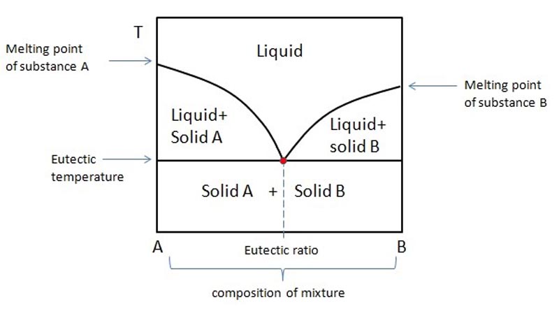
Typical molten salt mixture used for energy storage is represented by the ternary eutectic
53 wt % KNO3 (potassium nitrate)
40 wt % NaNO2 (sodium nitrite)
7 wt % NaNO3 (sodium nitrate)
or binary eutectic
45.5 wt % KNO3 (potassium nitrate)
54.5 wt % NaNO2 (sodium nitrite)
The eutectic temperature for those compositions is in the range 142 to 145 oC.
The molten salt is used for high temperature energy storage applications (above 400 oC) because typical thermal fluids, such as synthetic oils, have temperature limitation and decompose beyond the maximum allowable temperature (410-430 oC).
This is how the molten salt storage is employed in a solar thermal plant. First, the solar energy is caught by the collectors and concentrated on the receiver tube filled with heat transfer fluid. The heat transfer fluid (with temperature of ~393 oC) is circulated in a closed loop to deliver heat to the steam generator, which produces superheated steam, and then the thermal fluid flows back to the solar collectors (with temperature of ~ 293 oC). Such a loop can only operate during sunshine hours. To extend the steam generation beyond sunshine hours, molten salt thermal energy storage is used. The thermal storage usually consists of two salt storage tanks. In this case, the closed loop with the heat transfer fluid is passed through one of the salt tanks, where salt is heated to the temperature of ~ 384oC. The tank is insulated, so salt can stay hot for a substantial period of time (estimated heat loss ~0.5 oC per day). The molten salt is stored in the tanks at ambient (atmospheric pressure). To discharge heat during night hours, the molten salt from the hot tank is pumped through the steam generator to produce steam, and then to the cold storage tank (at ~ 292 oC). In this configuration, some part of the heat transfer fluid loop is diverted to the heat exchanger between the cold and hot salt tanks. The cooled molten salt is then pumped through the heat exchangers and returns to the hot salt tank.
Solar tower systems can use molten salt as heat transfer fluid and heat storage medium without involving any additional thermal transfer fluid loops due to higher radiation concentration temperatures. In this case, molten salt is flowing through the tower-mounted molten salt receiver, where it is heated to 565 oC. Then the salt is supplied to the hot salt tank, from where it flows to the steam generator. This concept is illustrated on the eSolar website [114].
In this case, the use of molten salt for both heat transfer and thermal energy storage minimizes the number of storage tanks and salt volumes needed.
The following video (~2 min) provides a simple illustration of the molten salt thermal energy storage concept.
Storing energy in fluids involves exchanging heat between different types of fluids in heat exchangers. For example, transfer of heat from a thermal fluid in solar-heated tubes to the molten salt reservoir requires a heat exchanger; further transfer of heat from the molten salt to water to produce steam would involve another heat exchanger. There is a thermal physics method to calculate the effectiveness of the heat transfer in different types of heat exchangers and to evaluate their performance. One example of such calculation is given in Section 3.17. of the book "Solar Engineering of Thermal Processes" by Duffie and Beckman (2013), referred to below.
Additional Reading
Book chapter: Duffie, J.A. and Beckman, W.A., Solar Engineering of Thermal Processes. Section 3.17 Effectiveness-NTU calculations for heat exchangers. pp. 168-170.
This reading is available online through PSU Library system. It is an optional material to study if you are interested in more insight in how heat is transferred from one medium to another, and what kind of losses can be expected. More thorough consideration of thermal topics is included in EME 811, which is also part of RESS Solar Option program.
Summary and Activities
Summary and Activities
Strategic planning of a CSP facility involves a number of steps - site evaluation, socio-economic assessment, environmental assessment, and system modeling and optimization. All these steps must be taken before investment is made, and work has begun. Feasibility analysis requires several iterations and special expertise to justify the decision. This lesson introduced you to a few useful tools and methods to start with.
After you have covered the assigned readings for this lesson, please complete the following assignments:
| Type | Description/Instructions | Deadline |
|---|---|---|
| Discussion Forum | Discussion Forum "Social benefits of solar thermal systems": Lesson 8 What, in your opinion, is the most important benefit of CSP technology for local economy and society in general?
|
Sunday night |
| Activity | SAM exercise
Note: I hope you are familiar with the SAM software, since it was used in your EME 810 course. If you are missing that prerequisite, go to this EME 810 page [115]to learn how to install and run SAM. |
Wednesday night |
References for Lesson 8
Lovegrove, K., Stein W., Concentrating Solar Power Technology, Woodhead Publishing, 2012.
NREL, 2013 / http://www.nrel.gov/docs/fy13osti/56290.pdf [110]
Eilbert, A., The Trade-Off Between Water and Energy: CSP Cooling Systems Dry Out in California, Revolt - Worldwatch Institute, 2010.
Caldes, N., Varela, M., Santamaria, M., and Saez, R., Economic impact of solar thermal electricity deployment in Spain, Energy Policy 37, 1628-1636 (2009).
Lechon, Y., de la Rua, C., and Saez, R., Life Cycle Environmental Impacts of Electricity Production by Solar thermal Power Plants in Spain, J. Solar Energy Eng., 130, (2008).
Lesson 9: Energy Storage Technologies for Solar Systems
Overview
Overview
This lesson will overview energy storage options for large-scale solar facilities. Clearly, energy demand rarely coincides with energy generation. Being bound to daily solar activity cycle at a certain locale, solar energy conversion systems are intermittent by nature, therefore, using energy at nighttime requires technologies to store energy on site. Photovoltaic systems, which convert natural solar resource into electric power, require means for electrical energy storage, while CSP systems may be better off storing thermal energy. The thermal storage principles and technology were discussed in the previous lesson, and Lesson 9 is primarily concerned with the technologies used to store electric power. For storage, electrical energy is often converted to other kinds of energy; for instance, potential mechanical, kinetic mechanical or chemical energy, which would be stored as fuel. Energy storage research has been accelerated over the recent years to address the need for compact and economically efficient storage technologies and is currently define the rate implementation of the commercial renewable energy systems. This lesson readings provide an overview and resources for learning the storage technology principles, with understanding that some of those options are much more advanced and rapidly evolving than others.
Learning Outcomes
By the end of this lesson, you should be able to:
- explain the technical principles of energy storage used in utility-scale solar plants;
- understand the performance metrics for storage systems;
- articulate technological, environmental, and economic cons and pros of energy storage implementation.
Readings
Book Chapter: Foster, A., Chassemi, M., and Cota, A., Solar Energy: Renewable Energy and the Environment. CRC Press, 2010. Chapter 11. Energy Storage, pp. 265-293.
Book chapter: Butler, P.S., Eidler, P.A., Grimes, P.G., Klassen, S.E., and Miles, R.C., Zinc/Bromine Batteries [116], in Advanced Battery Systems, pp. 37.1-37.15. Sandia National Laboratories, 2000.
Web article: Vanadium Redox Flow Batteries [117], Energy Storage Association (ESA), 2015.
DOE Fact Sheet: Wang, E., Vanadium Redox Flow Batteries [118], U.S. Department of Energy, Energy Storage Program, 2012.
Review paper: Blanc, C. and Rufer, A., Understanding the Vanadium Redox Flow Batteries [119], in Paths to Sustainable Energy, Dr Artie Ng (Ed.), ISBN: 978-953-307-401-6.
Web article: LaMonica, M., Compressed Air Energy Storage Makes a Comeback [120], IEEE Spectrum, 2013.
Book Chapter: Grimes, C., Varqhese, O.K., Ranjan, S., Light Water Hydrogen. The Solar Generation of Hydrogen by Water Photoelectrolysis, Section 2.2 Hydrogen Generation by Water Splitting. pp. 35-52.
9.1. Options for energy storage
9.1. Options for energy storage
Because solar energy supply is variable in time, energy storage is an important issue. Energy storage is used to collect the energy generated by the solar conversion systems (thermal or photovoltaic) in order to release it later on demand. This can be a situation when sufficient power is produced during the day, and stored energy is used during the night. Also, when insolation conditions are ideal, the solar system may produce enough power for the target application, but on dull days, direct energy supply from collectors is diminished, and the energy from the storage is used to compensate the deficit. Energy storage devices help to smooth out differences and minor fluctuations in energy supply caused by shading, passing clouds, etc. Development of efficient and cost-effective energy storage is considered the main bottleneck of the universal development of solar systems.
Video: How solar energy got so cheap, and why it's not everywhere (yet) (7:53)
Introduction
Narrator: Solar. It's astonishing. But clean energy from the sun. Solar energy has become the cheapest way to generate electricity. It's even cheaper than coal. And yet it produces only 3% of the world's electricity. Why aren't we using way, way more of it? How did it get so cheap? And what does all this have to do with ducks? Let's find out.
How solar energy got so cheap
Narrator: First, Let's take a look at how much the price for solar has fallen.
Jenny Chase, Head of Solar, BloombergNEF: I started this job as an analyst of solar in 2005, and then I thought, solar is ridiculously expensive.
Narrator: Jenny Chase is the head solar analyst at research firm Bloomberg NEF.
Jenny Chase: You'd pay about pay about $4 a watt for a solar panel, and today you'd pay about $0.20 for that same watt.
Narrator: And that is just the last 15 years. If you look further back, the price drop is even more impressive. How did this happen?
Gregory Nemet, Author, “How Solar Became Cheap”: It's been a long story, but it's unbelievable.
Narrator: Gregory Nemet has written a book about this.
Gregory Nemet: No one country did it. It was an exchange of one country building on another. One, the US created the technology.
Narrator: The modern day solar cell, made from silicon, was invented in the US in 1954. Back then, it mainly got used in the space industry and was still super expensive. But as the technology progressed, prices started to fall.
Gregory Nemet: Two, Germany created a market.
Narrator: In 2000, Germany passed a law to boost renewable energy development. This was big because it put a fixed price on energy generated from sources like wind or solar. That gave people and companies a reason to set up solar panels. And for them to do that, someone needed to build these solar panels.
Gregory Nemet: Three, China made it cheap.
Narrator: Once the German Lohat came into force, China really started to pump out those solar cells.
Jenny Chase: So basically, it built a whole industry for this on a scale that the west really didn't keep up with.
Gregory Nemet: China was almost a nonexistent player 20 years ago, and today they're the biggest producer of solar panels, about 70% of the world's production.
Narrator: So this is how we ended up where we are now, with clean energy. That also makes business sense. But if solar is so great, why don't we rely on it much, much more and just switch off all these dirty power plants? Well, solar has always had this one big problem. It only really works when the sun is shining, when it's cloudy, or even worse, dark. Even the best solar cells are pretty useless. And that's a real shame, because that's when we'd need them the most. Let's take a look at how we use energy. In the morning, when most people get up and get ready. We need energy. The so-called duck curve charts our demand for power from nonrenewable sources like coal and gas, throughout the day, first, in places without much solar. After the morning spike, it stays pretty level. When people come home in the evening, it goes up again and then drops at night. At this point, you might get an idea why they call it the duck curve, because it kind of looks like a duck. Anyway, in places with lots of solar, like California, this curve changes. The mornings are pretty much the same.
Then the sun rises and solar energy production kicks in. This lets demand for non renewable energy drop until the sun sets, that is. That is when conventional demand shoots up again, way steeper than in the first curve. Two problems with this. One, traditional power plants suck at ramping up this quickly. That means you have to keep them running at a certain output all day, even though there's lots of solar. And that means….
Jenny Chase: That you can end up with actually more power produced in the middle of the day than is used.
Narrator: And that leads to the second problem. There are limits to how much energy you can put into the grid. Too much solar could overpower it, so it needs to be thrown away. This has always made it super difficult to add lots of solar to power systems. But guess what? There is now a solution to this, and chances are you have part of it in front of you right now. A lithiumion battery.
Lithiumion batteries
Gregory Nemet: We're just taking that same construction, stringing together many, many of those cells, and making battery packs that we can use for cars. And then we can also scale that up to use for stationary power to go next to wind parks or solar farms.
Jenny Chase: What's been quite good over the last few years is that batteries have got a lot cheaper as well. And we're now seeing solar projects built with a couple of hours of storage in the battery, so that they could shift solar generation from the middle of the day to the evening, where there's often a peak in electricity demand.
Narrator: In the US, for example, the state of New Mexico just decided to shut down a coal plant and instead build new solar farms that store large amounts of the energy they produce in batteries. Lithiumion batteries have become a lot better and a lot cheaper than expected in the last few years. They're now a viable option for storing and shifting at least a few hours worth of solar energy as needed. So the storage problem that solar always had is actually not that much of a problem anymore. Sometimes, though, we might want longer term storage in places without much sunshine, for example. And that's why companies are offering other solutions. Let's just run through a few.
Alternatives
Narrator: Another type of battery, called a flow battery, separates the charge outside a cell. That has two advantages. It can store more energy and for longer. The problem is they're still relatively expensive. Then there's pumped hydro storage, which is already used quite a bit. You need two lakes, and one of them needs to be in a hill. During the day, you use solar energy to pump water from the lower lake up to the higher lake. When you need energy at night, you can just let it run down through a turbine.
But for that you need to find lakes and, well, a hill. Another solution using gravity comes from a swiss company. It's working on a tower that raises building blocks with solar energy and then releases the energy by lowering them again. But for this too, you need space. And there's also the option of using solar to produce hydrogen. And with that hydrogen, you could then do a number of things like fuel cars, or even make steel. But the whole process is still pretty costly.
Jenny Chase: I think that the storage will mostly be lithiumion. With some hydrogen and maybe a few other options.
Gregory Nemet: There are alternatives. It's just that lithiumion batteries are becoming so flexible and so inexpensive that it'll be hard for these alternatives to compete them. But they do have other attributes, like they hold a charge longer, which could turn out to be play a pretty important role in some applications.
Narrator: Solar has become cheap and has pretty much fixed its biggest problem. So what's next?
Jenny Chase: It's going to be big. It's going to be everywhere. We forecast that even with no further policy, solar would supply about 23% of global electricity by 2050. I personally think it's going to be much higher than that.
Gregory Nemet: I would not be surprised if by 2030, we're talking about solar doing a large part of the world's electricity supply.
Narrator: Solar has come a long, long way. But now that the technology is in place, it really looks like it's time to shine. Now we'd like to hear from you. What are your thoughts on solar energy? Let us know in the comments. And hit subscribe for more videos like this every Friday.
There are quite a few different technology options for energy storage, which are briefly outlined below:
- Grid. For grid connected solar systems, the most natural and cost-effective way would be to store energy in the grid. The main idea here is that the DC power from a solar facility (array or farm) is converted to AC power and is fed to the grid and further on is used for on-site or off-site applications. This way, the grid acts as the medium that collects energy from different power-making facilities (renewable or non-renewable) and redistributes it as necessary. Since a grid does not really represent a separate system that is part of a solar plant, it will not be discussed further in this lesson.
- Fluid. Fluid-based storage is typically used with solar thermal systems. Unlike grid, which stores electrical energy, fluids store thermal energy. Fluids, such as water, oil, molten salt or others act as a medium for absorbing heat. The main idea is that the solar radiation heats the heat-transfer fluid which is accumulated in the tank. The tank is insulated, so the hot fluid keeps its temperature for a substantial period of time. When needed, the heated fluid is used in a heat-exchanger to produce steam for the electric generator. This type of thermal energy storage was discussed in more detail in Lesson 8.
- Battery. A battery is an electrochemical device that stores chemical energy in internal components and releases energy as electricity, which is generated through electrochemical reactions. Batteries are reversible, i.e., can be charged and discharged, and the parameters of these processes are regulated to avoid damage by overcharging or over-discharging. Battery life is expressed in number of charge-discharge cycles. There are many different types of batteries, some of which will be discussed further in this lesson.
- Hydrogen. The idea behind hydrogen storage is that electricity generated by solar PV systems can be used to electrolyze water - to split it to hydrogen and oxygen. Further, hydrogen gas is collected and can be used as a fuel. One of the highly efficient devices "converting" hydrogen back to electricity is H2/O2 fuel cell, which has zero carbon footprint during operation.
- Compressed air. In this case, the electrical energy produced by a PV solar system is used to run compressors to compress massive amounts of air and store it in underground, above-ground, or underwater containers. Later on, when energy is needed, the air is decompressed and is supplied to a turbine to generate electricity. Compressed air energy systems (CAES) promise high efficiencies, although this technology is not yet widely implemented.
- Pumped storage hydropower. The available energy can be used to pump water into an elevated reservoir for storage. When power is needed, the water can be discharged under gravity to run a turbine, which is connected to a generator to produce electricity. The same as compressed air systems, the pumped storage technology has high energy return on investment, although it may require special topographical conditions and water availability in order to be used.
All of the above options for energy storage should be employed with understanding the facility needs and capacity. What energy storage is efficient for small residential systems may be insufficient or too costly when scaled up to the utility-size systems. Determining capacity of energy storage for a particular solar project is an important technical and economic issue. For example, if the capacity of the storage is too large compared to the energy produced by the solar conversion facility, the total system cost will be unnecessarily increased. On the contrary, if the capacity of the storage is too small, that leads to energy dumping and overall unsatisfactory plant performance.
In the following sections, we will discuss different energy storage options that can be possibly applied to utility scale solar systems.
9.2. Battery storage
9.2. Battery storage
Batteries are commonly used to store electric energy generated by off-grid renewable energy systems, and also to mitigate the sharp fluctuations of power for on-grid systems. While there are many different types of battery technologies, some are more applicable to utility scale energy storage than others. Applicability to large systems depends on such factors as cost of materials, ability to scale up with no ill effects or performance loss, and design and operation mode.
Some well-known examples of battery types used as stationary storage system for PV solar are listed in Table 9.1
| Technology (battery type) | Power subsystem cost $/kW | Energy storage subsystem cost $/kW | Charge-discharge efficiency % | Cycles |
|---|---|---|---|---|
| Advanced lead-acid | 400 | 330 | 80 | 2,000 |
| Sodium/sulfur | 350 | 350 | 75 | 3,000 |
| Lead-acid with carbon enhanced electrodes | 400 | 330 | 75 | 20,000 |
| Zinc/bromine | 400 | 400 | 70 | 3,000 |
| Vanadium redox | 400 | 600 | 65 | 5,000 |
| Li-ion (large) | 400 | 600 | 85 | 4,000 |
| Flywheels (high-speed composite) | 600 | 1,600 | 95 | 25,000 |
| Super capacitors | 500 | 10,000 | 95 | 25,000 |
Note: The costs in the table are based on standard assumptions for the applications and technologies considered, and on expert opinion. They are meant to be used for comparative purposes. The actual costs of any storage system depend on many factors and the assumptions and the means of calculating some of the values are subjective and continue to be debated, even among experts in the field (Sandia National Laboratories).
For quite a while, lead-acid batteries have been the first choice for off-grid PV applications. This lead-acid battery technology has been around since the 19th century and, historically, service providers have more knowledge and tools to deal with those systems. But, despite their long existence and widespread use, lead-acid batteries remain one of the lowest energy-to-weight and energy-to-volume battery designs, which means they are too big and heavy for the amount of energy they provide. This technology is inexpensive and reliable, and it may be a while before it is replaced by more advanced types on a wide scale.
The following reading provides more information on the battery storage types and lead-based batteries, specifically.
Reading Assignment:
Book Chapter: Foster, A., Chassemi, M., and Cota, A., Solar Energy. Renewable Energy and the Environment. CRC Press, 2010. Chapter 11. Energy Storage, pp. 265-293. (See E-Reserves via the Library Resources tab.)
Li-ion battery technology
Li-ion battery is one of the rapidly advancing technologies preferred for employment in conjunction with solar systems due to high storage capacity, high charging rates, light weight, and relatively long service life. However, the technology cost is still high and can be a limitation on the utility scale. Some of the very attractive features of Li-ion batteries are high power output and high charge-discharge efficiency. They can also withstand more charge-discharge cycles than lead-acid batteries.
The principle of operation of the Li-ion battery is discussed below.
A schematic representation of a generic Li-ion battery is given in Figure 9.1. Roughly, Li-ion cell consists of three layers: electrode 1 (cathode) plate (usually lithium cobalt oxide), electrode 2 (anode) plate (usually carbon), and a separator. The electrodes inside the battery are submerged in an electrolyte, which provides for Li+ ion transfer between the anode and cathode. The electrolyte is typically a lithium salt in an organic solvent.
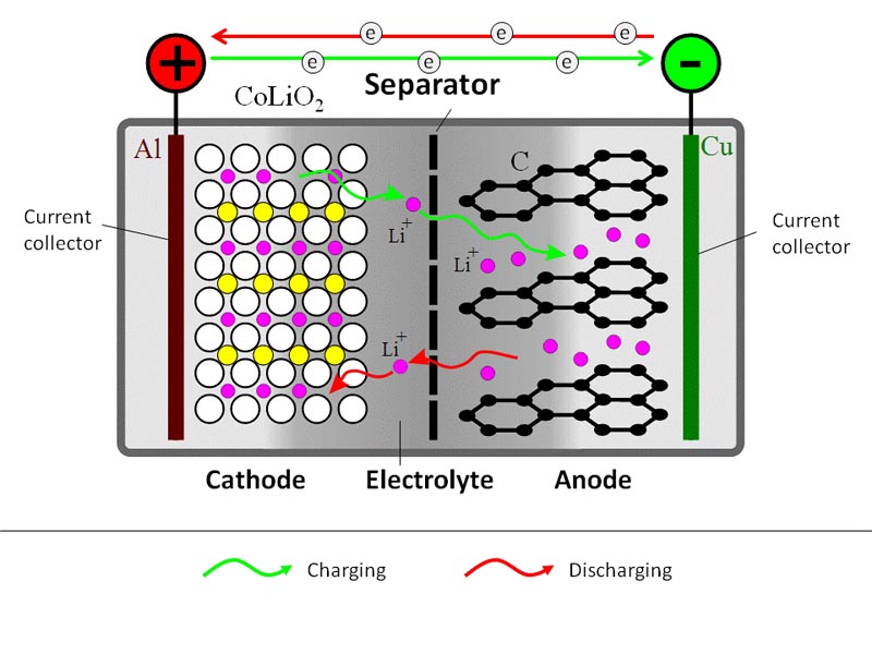
During the charging process, a DC current is used to withdraw Li+ ions from the cathode and to partially oxidize the cathode compound:
LiCoO2 → Li1-xCoO2 + xLi+ + xe–
The released Li+ ions migrate through electrolyte towards the anode, where they become absorbed in the porous carbon structure:
xLi+ + xe– + C6 → LixC6
At the same time, electrons travel through the external circuit (electrolyte is not electron conductive).
During the battery discharge, the reverse process takes place. Li+ ions spontaneously return to the cathode, where electrochemical reduction occurs.
Limitations of the Li-ion batteries are rooted in the material properties.
For example, the LiCoO2 ⇔ Li1-xCoO2 conversion is only reversible with x<0.5, which limits the depth of the charge-discharge cycle. But with a wider variety of materials available, research is underway to develop new generations of Li-ion batteries.
For example, take a look at the Sigma Aldrich [122] website, which lists multiple alternatives for cathode, anode, electrolyte, and solvents.
| Advantages | Limitations |
|---|---|
| 1. Relatively high energy density and potential of finding even better formulations. | 1. Circuit protection needed to avoid damaging high voltage / current. |
| 2. No need for priming - new battery is ready to operate. | 2. Aging - battery gradually loses its capacity even if not in use. |
| 3. Low self-discharge (compared to other types of batteries). | 3. Toxic chemicals are subject to regulations. |
| 4. Low maintenance. | 4. High cost of materials and manufacturing process. |
| 5. Capability to generate high current / power. | 5. Technology is not fully mature; varying components and chemicals. |
Supplemental reading on the status of Li-ion battery technology:
Goodenough, J.B. and Park, K.S., The Li-Ion Rechargeable Battery: A Perspective, J. Am. Chem. Soc., 2013, 135 (4), pp 1167–1176.
Etacheri, V., Marom, R., Elazari, R., Salitra, G., and Aurbach, D., Challenges in the development of advanced Li-ion batteries: a review, Energy & Environmental Science, 2011 (9), 3243-3262.
Flow Batteries
Flow batteries, unlike solid-state batteries, have their chemical components dissolved in liquid solutions, which can be pumped through the electrodes in a flow. If you are familiar with the concept of fuel cell, it is something similar in principle of operation, although it is still a closed loop system. A flow battery cell itself can be small, while the solutions can be contained in external storages. One of the advantages of the flow batteries is almost instant replacement of the electrolyte liquid, thus eliminating any gradient or concentration fluctuations at the electrodes. The main difference between the conventional batteries and flow batteries is that the energy is typically stored in the liquid phase in flow batteries. So, increasing the size of the storage tanks for the liquids allows easy scale-up of the battery to match a specific application.
Zinc-bromine flow battery storage
Zinc-bromine battery is a type of hybrid flow battery. It uses zinc bromine as the working solution, which is stored in two compartments, separated by a porous membrane. One compartment has a negative zinc electrode and the other compartment has a positive bromide electrode. During charge, supplied electricity (e.g., from a solar conversion system) is used to electroplate metallic zinc (Zn) on the negative electrode, while bromine (Br2) is generated on the positive electrode. During discharge, the opposite process occurs: Zn is dissolved to form Zn2+ ions in solutions, and bromine is converted back to bromide ions (Br-).
Here are the electrochemical reactions involved in this process:
Zn2+ + 2e- → Zn(s) - Reduction of zinc during battery charging
2Br- → Br2(aq) + 2e- - Oxidation of bromine during battery charging
The overall reaction is therefore:
Zn2+ + 2Br-⇔ Zn(s) + Br2(aq)
This reaction proceeds to the right on charging and to the left on discharging. The standard electrode potential for the overall reaction is 1.85 V, which is the maximum theoretical voltage that can be expected from a single cell. The battery cells are stacked to increase the overall storage capacity of the system.
The battery compartments are made of inert plastic. Unlike common batteries, which store electrolyte within the reaction chamber, zinc-bromine batteries have solution storage in the external tanks, from where it is circulated through the electrodes (flow battery type). The external bromide solution storage also helps maintaining required concentration of bromide throughout the reaction cycle.
This technology has been commercialized by ZBB EnerStore company, which engineered zinc-bromine batteries into 50 kWh modules, scalable up to bigger storage systems. Each module is a stand-alone system that includes all necessary software and hardware. Some advantages of this technology include high-energy density (75-85 Wh/kg), stability, i.e., good resistance to performance degradation, ability to operate at full output within a wide temperature range. Unlike most batteries, ZBB EnerStore batteries use non-reacting electrodes (i.e., electrodes are not reactants, but simply are substrates for reactions to take place), which helps minimize loss of performance from repeated cycling.
Watch this video (5:19 minute) for a demo of ZBB EnerStore solution for zinc bromide battery technology:
Video: ZBB EnerStore (5:19)
PRESENTER: Introducing ZBB EnerStore, ZBB Energy's third generation flow battery. ZBB has completely re-engineered its zinc bromide flow battery to be the most advanced and cost effective energy storage device for distributed energy projects, whether on or off the grid. The new design is easy to maintain and operates indoors or outdoors in the widest ambient temperature range of any flow battery, so there are no additional costs associated with constructing and maintaining a climate-controlled building. ZBB EnerStore batteries are self-contained, modular units and are easy to transport, so we can deliver an expandable solution that is virtually plug and play at your site with no on-site wiring needed. Although there are many different energy storage options to consider when compared to lead acid batteries, ZBB's flow batteries have a higher energy density, the lowest cost of ownership over a 20-year lifespan and are the most effective way to maximize the use of renewables. By utilizing energy storage with renewable power sources, diesel gensets can be configured to operate in backup mode only, reducing run time and fuel consumption, and you don't need to worry about the complexities of federal emission compliance. ZBB flow batteries are also "black start" capable. Most other energy storage systems need the grid to work. The ZBB EnerStore flow battery is well-suited for a variety of commercial applications with or without renewable energy sources and is readily configurable and scalable.
The ZBB EnerStore battery is built in 50 kilowatt hour modules and expandable to 500kWh in a singular enclosure. With multiple enclosures linking together, it can contain up to 2 megawatt hours or more on a single point of connection. Each battery module is comprised of eight cell stacks with 60 cells each, DC to DC converters, a self-regulating heat exchanger, electrolyte storage tanks, and built-in secondary spill containment. With ZBB's innovative, integrated DC bus architecture and converters on each module, there are no voltage limitations or concerns about system design and operation. In addition, ZBB's flow batteries operate without any special ventilation requirements. Since flow batteries are made with inert materials, they are safe to install. Electrolytes are never handled or replaced, only the cell stacks are changed out over the course of its life cycle. ZBB's flow batteries are environmentally friendly, made with highly-recyclable materials and recoverable at the end of their service life. Now let's take a look at how the zinc bromide battery works. ZBB's flow battery technology is based on the reaction between two readily available chemicals, zinc and bromine. The battery consists of a zinc anode and a bromide cathode, separated by a microporous separator. The aqueous solution of zinc bromide is circulated through the two compartments of the cell from two separate reservoirs.
During charge, electricity causes a reaction with the zinc bromide solution to electroplate zinc and form bromine on the battery electrodes. The reaction is reversed during discharge. The zinc and bromine reacts electrochemically to produce electricity while reforming the zinc bromide solution. Circulation pumps are used to allow the zinc and bromide to flow continuously throughout the cell stacks. While the electrolyte is flowing, an onboard computer calculates the state of charge of the battery module and directs when energy should be stored or if the stored energy should be discharged. An inline heat exchanger regulates the temperature of the battery module and keeps it within the standard operating range regardless of ambient temperature or rate of charge and discharge operation. The ZBB EnerStore can be left indefinitely at any state of charge, from 100% to completely discharged. The ZBB EnerStore battery is your answer for capturing multiple value streams, from time shifting, to firming of renewables or load management, to system backup. It's the best choice over a 20-year cost of ownership. Using EnerStore as part of ZBB's integrated management platform provides a continuous supply of energy and optimizes all of your interconnected resources, no matter your energy source or connection to the grid. ZBB, optimizing energy availability.
Reading Assignment
Learn more on Zn-Br battery technology:
Book chapter: Butler, P.S., Eidler, P.A., Grimes, P.G., Klassen, S.E., and Miles, R.C., Zinc/Bromine Batteries [124], in Advanced Battery Systems, Sandia National Laboratories, pp 31.1-37.15. (See E-Reserves via the Library Resources tab).
Vanadium Redox Flow Batteries
This type of battery utilizes the multiple redox states of vanadium (V) in its charge-discharge cycles. Vanadium is present in the dissolved form in the sulfuric acid medium, and because it is all-vanadium system, this type of battery is not susceptible to performance loss due to cross contamination.
During charging, the following half-reactions occur in two separate compartments of the battery:
V3+ + e– → V2+
VO2+ + H2O → VO2+ +2H+ + e–
Electrons are supplied from the solar energy conversion system as DC current onto non-reacting electrode dipped in the V3+ solution. As a result, V3+ is reduced to V2+. At the same time in the other compartment, vanadium (IV) species VO2+ is oxidized to vanadium (V) species VO2+, releasing the electron. On discharging, these reactions are reversed.
The summary process is expressed through the following reaction:
VO2+ + V3+ + H2O ⇔ V2+ + VO2+ + 2H+
The total voltage generated by a single vanadium redox flow battery is around 1.25 V in ideal case.
The main benefits of the vanadium redox flow batteries ability to go through "unlimited" number of cycles; they have a long lifespan (>20 years), quick charging, and high efficiency of the charge-discharge cycle (~80%). They are also more environmentally friendly in terms of component toxicity than many other types of batteries.
Reading Assignment
The following sources will help you to better understand the technical details of the vanadium redox batteries, as well as its challenges.
DOE Fact Sheet: Wang, E., Vanadium Redox Flow Batteries [118], U.S. Department of Energy, Energy Storage Program, 2012.
The vanadium redox flow battery technology is potentially suitable for extra-large utility scale applications. For example, the 200 MW VRB battery facility in Dalian, China, is expected to significantly increase the stability of the electric grid by supplying power during peak hours and emergency black-starts. Development of such a mega facility was enabled by its co-location with the VFB cell manufacturing factory, which is tapping into local vanadium resources. The Dalian battery is expected to become operational in 2020. Nearby wind power facilities have been forced to curtail electricity production – this battery facility hopes to reduce curtailing significantly.
Check out the story here [125].
Probing question
Will the Dalian energy storage facility become truly the largest battery in the world when brought online? What is the capacity of the largest Li-ion Battery storage built to date, and how does that compare?
Additional resources:
Review paper: Blanc, C. and Rufer, A., Understanding the Vanadium Redox Flow Batteries, in Paths to Sustainable Energy, Dr. Artie Ng (Ed.), ISBN: 978-953-307-401-6. pp. 333-337(Access the article in Canvas).
This paper is quite technical as it describes different models used to analyze the performance of the vanadium redox flow batteries. Read sections 1 and 2, which describe the electrochemical principles behind the battery operation. Reading further sections may be useful if you have a special interest in this topic, but is not required.
9.3. Compressed Air and Pumped Hydro
9.3. Compressed Air and Pumped Hydro
Compressed Air Storage
Compressed air storage technology may become an efficient solution of storing energy generated by large solar plants. The concept is as follows.
Air is used as the energy transfer medium. During the daytime, solar power is used to heat and compress air in an airtight chamber. When energy is needed, that compressed air can be expanded through a turbine or another expansion device to drive a generator to create electricity. Compressed Air Energy Systems (CAES) have been in use in some conventional power plants, and they are making a come-back as energy storage systems for renewable energy plants.
Traditionally, CAES technology used underground geological formations, such as salt caverns, as reservoirs for compressed air. While this approach was effective at some locations, it was not universal, as geology in some areas may be just unsuitable. A newer approach with CAES is to use human-made chambers - large pipes, such as those used for natural gas pipelines. While it involves more construction and installation, this type of artificial storage can be employed virtually anywhere and scaled up to the required capacity by simply using longer pipes.
Reading Assignment
Please read the following review to understand the basic principles and cons and pros of CAES:
Review article: Wang, J., Lu, K., Ma, L., Wang, J., Dooner, M., Miao, S., Li, J., and Wang, D., Overview of Compressed Air Energy Storage and Technology Development [126], Energies, 2017, 10, 991.
Please read the following article to learn about the new approach in CAES technology:
Web article: LaMonica, M., Compressed Air Energy Storage Makes a Comeback [120], IEEE Spectrum, 2013.
This article explores the idea of underwater compressed air storage, which may become an efficient storage solution for solar plants located near the coastline.
Web article: Dorminey, B., Underwater Compressed Air Energy Storage: Fantasy or Reality? [127] Renewable Energy World, 2014.
Based on this reading, answer the following self-check questions:
Check Your Understanding Question 1 (Multiple Choice)
Check Your Understanding Question 2 (Essay)
Why is some amount of natural gas needed in traditional CAES systems?
Check Your Understanding Question 3 (Multiple Choice)
Pumped Hydro Energy Storage
Pumped-storage hydropower (PSH) is the type of storage technology that is based on storing energy in the form of potential energy of water. It consists of two water reservoirs at placed at different elevations connected by discharge channel. The available energy can be used to pump water to the upper reservoir (recharge phase), and energy is released when water moves back down to the lower reservoir through the turbine (discharge).
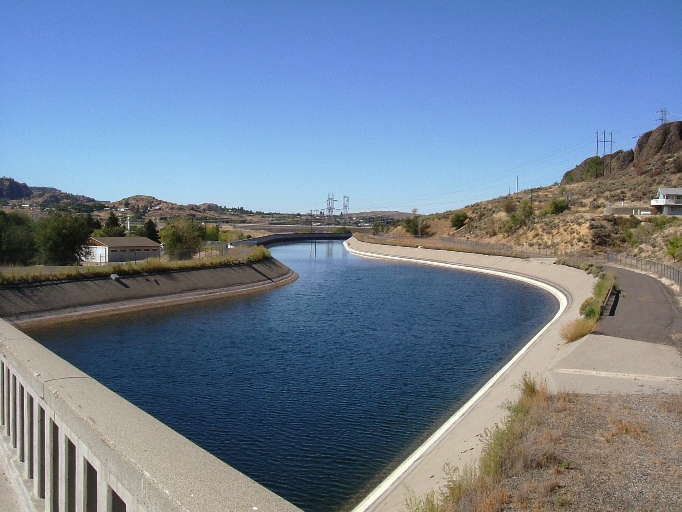
_(2).jpg)
Closed loop PSH storage does not need to be connected to an outside natural body of water, and all the water is re-circulated.
This storage technology is not new. The first commercial systems employed for storage were implemented in the 1970s, and the design changed very little since then. According to U.S. DOE, pumped-storage currently accounts for 95% of all utility-scale energy storage in the United States. However, additional investments are considered in innovative pumped storage technologies to explore its potential for storing non-dispatchable renewable power generated from utility scale wind and solar farms and improving grid resiliency and reliability.
Listen to the recent podcast that discusses the potential of various energy storage options for utility scale renewables:
What to do you think? Which method of those mentioned in the discussion has a better chance to become the main player for storing mega- and giga-amount of power?
9.4. Hydrogen storage
9.4. Hydrogen storage
In this section, we will discuss how solar energy can be stored in the form of hydrogen gas. Hydrogen (H2) is a common industrially used chemical and fuel, which can be obtained from water by electrolysis or by reforming of natural gas. Electrolysis is of special interest in the energy storage context, since it converts electric energy into something storable. The process of electrolysis involves passing electric current through water or another aqueous solution, which initiates the electrochemical reaction:
H2O ⇔ H2 + 1/2O2
The basic idea is that the electricity generated by solar PV systems during daytime can be used to run electrolyzers to split water into hydrogen and oxygen gases. Hydrogen is collected and stored in one or another form. When energy is needed, hydrogen can be used for combustion or for electrochemical conversion (in a fuel cell) to recover energy as heat or electricity. Hydrogen provides a new form of energy economy, which complies with the present-day environmental requirements. For instance, hydrogen combustion does not result in any carbon emissions, and water and heat are the only products. Electrochemical utilization of hydrogen in fuel cells is thermodynamically efficient and environmentally benign. Fuel cells can be used for both stationary power generation and transportation. Unlike other forms of energy storage, hydrogen can be transported and used at a different location.
There are a few advantages of the hydrogen energy storage in solar plants:
- Hydrogen generation by electrolysis is a well-established technology. Hydrogen is used in multiple branches of industry, so the procedures for its handling are well developed.
- Water electrolysis uses low-voltage DC current, which is compatible with the output from the PV cells.
- Hydrogen can be stored with minimal losses.
- Hydrogen can have multiple uses - electricity generation, heat and power generation.
- Hydrogen is an environmentally benign substance, its combustion does not produce harmful emissions, it is volatile and is easily dissipated.
- There are multiple ways of hydrogen transportation (pipelines, tanks, hydride compounds).
- Existing infrastructure for natural gas can be adapted to hydrogen use.
Electrolysis
There are different types of electrolysis that can be used for hydrogen generation. All of those methods use the available electricity to drive otherwise non-spontaneous electrochemical reaction. Electrochemical cell is required to realize electrolysis process. A typical electrochemical cell for electrolysis consists of two electrodes connected to an electric circuit submerged in the working solution. The electrode compartments are separated from each other with a gas-impermeable membrane, which does not allow hydrogen and oxygen mix, while allowing conduction of ions.
Use the following reading material to learn the scientific background and engineering principles for different electrolyzers.
Reading Assignment
Book Chapter: Grimes, C., Varqhese, O.K., Ranjan, S., Solar Production of Hydrogen by Water Electrolysis, Section 2.2 Hydrogen Production by Water Electrolysis. pp. 35-52. (See E-Reserves via the Library Resources tab.)
Note on hydrogen safety
Due to high reactivity, hydrogen storage brings up some safety issues. At certain conditions, reaction between hydrogen and oxygen can lead to explosion (Figure 9.4), so storages for those gases should be separated, and leak detection is critical.
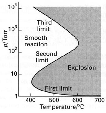
Solar hydrogen is attractive due to its carbon-free footprint, in contrast to any hydrocarbon fuels. Hydrogen has a very high energy density (142 MJ/kg), which is much higher than that of gasoline (~47 MJ/kg). This is due to its very light atomic mass. On the other side of the medal, hydrogen as a volatile gas must be contained in a compressed form, and the traditional gas cylinders used for storage and transportation of hydrogen have been a concern. Such cylinders, usually about 35 kg in weight contain only 700 g of hydrogen (at 200 bar of pressure), which is equivalent to only 2.85 liters of gasoline (Komoto et al., 2009).
The production of hydrogen via water electrolysis is most relevant to utility-scale PV systems. The efficiency of the electrolyzer is above 75% at optimized conditions. Even higher efficiencies are promised at elevated pressure, although in this case extra energy needs to be spent for isothermal compression. Much more than production, hydrogen "packaging", i.e., converting it to a convenient form for storage, can be much more costly and energy-expensive. These forms include (1) compressed hydrogen, (2) liquefied hydrogen, and (3) metal hydrides.
In option (1), compressed hydrogen is much more usable compared to that at atmospheric pressure due to much higher energy density (2.54 MJ/liter at 200 bar versus 0.0127 MJ/liter at 1 atm) (Komoto et al., 2009). Further compression to 800 bar brings its energy density to 10.1 MJ/liter - close to that of liquid hydrogen. However, multistage compression is estimated to take up to 8-12% of the total energy that hydrogen contains as fuel (referring to higher heating value), and mechanical and electrical losses can increase this value even further. Option (2), hydrogen liquefaction requires even more energy - 30 to 50 MJ/kg hydrogen converted. Option (3), metal hydrides are special compounds that can bind hydrogen by forming chemical bonds under certain temperature and pressure conditions and release hydrogen when temperature and pressure change. Simple physical pressurizing hydrogen into hydride form is possible, but is not very attractive due to the large amount of metal hydride needed (50 kg per 1 kg H2 stored) (Bossel, 2006). Chemical binding of hydrogen in metal hydrides is much more promising.
Some examples of hydride compounds are CaH2, MgH2, LiH, NaAlH4, LiAlH4. Because metal-hydrogen bonds are quite strong, energy input is needed to release hydrogen from hydride. So, temperatures for hydrogen generation need to be raised to 120-200 oC. Nevertheless, the hydride storage is theoretically more efficient. For example, if we consider the reaction
CaH2 + 2H2O => Ca(OH)2 + 2H2 - reaction of hydride with water,
we can see that by molar ratios, 42 g of CaH2 release 4 g of H2(gas), so it is roughly 4:1 ratio; at the same time, compressed storage in the cylinder provides storage of only 1 kg of hydrogen per 50 kg of storage tank, i.e., 50:1 ratio. Because of the obvious advantage of the metal hydride, substantial research effort is underway to improve this technology.
Summary and Final Tasks
Summary and Final Tasks
In this lesson, we looked at very different technologies used to store solar energy. Those technologies differ in physicochemical principles, scale, and impact, and require quite different scientific and engineering background for detailed analysis. In that sense, this material is challenging. At the same time, it is important for solar specialists to be aware of various energy storage options, as well as recent innovations, and to be able to apply those options to specific conditions. Hopefully, this lesson has been a good step in that direction and will motivate you to learn more and to elevate your expertise down the road.
Please complete the following activities to complete this lesson.
| Type | Description/Instructions | Deadline |
|---|---|---|
| Readings | Complete all necessary reading assigned in this lesson. | |
| Discussion Forum | Discussion Forum "Store or not to store"
|
Sunday night |
|
Reading Quiz |
Complete the Lesson 9 Quiz. |
Wednesday night |
References for Lesson 9
Moens and Blake, 2004, Advanced Heat Transfer and Thermal Storage Fluids, Conference Paper NREL/CP-510-37083 January 2005, National Renewable Energy Laboratory.
Wu, B., Redy, R.G., and Rogers, R.D., NOVEL IONIC LIQUID THERMAL STORAGE FOR SOLAR THERMAL ELECTRIC POWER SYSTEMS, Proceedings of Solar Forum 2001 Solar Energy: The Power to Choose April 21-25, 2001, Washington, DC.
Koning, S., Molten Salt Systems Other Applications Link to Solar Power Plants [130], Bertrams Heatec Inc. Pratteln, Switzerland, 2007.
Solar Reserve, Molten Salt Energy Storage [131], 2015.
CalFinder, Compressed air the secret to solar energy storage, [132] 2015.
D. Shriver and P. Atkins, Inorganic Chemistry, Freeman, NY, 1999.
Komoto, K., et al., Energy from the Desert, Earthscan 2009.
Bossel, U, Does a hydrogen economy make sense? Proceedings IEEE, v. 94, no. 10, pp. 1826-1837 (2006).
Lesson 10: Utility Scale Solar + Storage
10.1 Purpose and Function of Utility Scale Storage Systems
Purpose and Function of Utility Scale Storage Systems
Energy storage technologies are expected to enable of electric grid modernization, addressing the current limitations of electricity infrastructure and increasing grid stability and resiliency. We can identify a number of critical functions that we expect the energy storage systems to perform.
- Integration of renewable energy into the electricity grid
The variability of solar and wind power makes it hard for electricity providers to plug them into the electricity grid. Grids constantly balance the supply and demand of electricity and thus benefit most from dispatchable sources of energy (so far fossil fuels that could be burned on demand provided that sort of convenience). Energy storage makes the solar and wind energy more dispatchable (available on-demand of grid operators) and hence more competitive with traditional fuel options.
- Addressing peak demand
Responding to peak demands requires the ability to generate power quickly. The traditional choice for peak power generation are natural gas turbines. The energy stored in the batteries is immediately available and can be used to meet peak demand. This helps use the renewable power for peak generation and avoid grid disruptions or blackouts.
- Time shifting
PV Solar panels generate power only during the daytime, with the peak at noon hours, while the peak energy demand is often located during evening hours, when the solar irradiation is low. So the solar power needs to be “time-shifted” to be available during the time of high demand, and this can be achieved by means of utility scale storage.
- Energy autonomy and independence
For communities living in areas without access to electricity grid, combined renewable energy plus storage systems may be the best option to provide for constant supply of electricity. This autonomous approach can be realized at both distributed (house / community) and utility (area / region) scales.
Probing Question
Can you think of other major purposes or functions provided by energy storage systems? What other services to industry and community can we expect from the storage technology development in the future?
Check out Table 10.1, which provides more detail on how storage systems serve the grid and help diversify the energy resources.
| Role | Time scale(s) | Description | Benefits to RE integration | Examples of EES technologies |
|---|---|---|---|---|
| Time shifting / Arbitrage / Load levelling | Hours to days | EES allows storage of off-peak energy and release during high-demand period | A solution to diurnal generation cycles that do not match load cycles | NaS batteries, CAES, PHS, RFB |
| Seasonal shifting | Months | EES stores energy for months at a tie, releasing it at times of the year when RE output is typically lower | Allows use of renewably-generated energy year-round reducing reliance on traditional generation in seasons with, e.g., low sunlight | Hydrogen, SNG |
| Load following / Ramping | Minutes to hours | EES follows hourly changes in demand throughout the day | May mitigate partial unpredictability in RE output during critical load times | Batteries, flywheels, PHS, CAES, RFB |
| Power quality and stability | < 1 second | Provision of reactive power to the grid to handle voltage spikes, sags and harmonics | Mitigate voltage instability and harmonics caused or exacerbated by uncontrollable variability of capital RE generation | LA batteries,NaS Batteries, flywheels, RFB |
| Operating reserves | ||||
| Frequency regulation | Seconds to minutes | A fast-response Increase or decrease In energy output to stabilize frequency | Mitigate uncontrollable moment-to-moment variability in RE generation output | Li-ion Batteries, NaS Batteries, Flywheels, PHS (with advanced variable speed control) |
| Spinning Reserves | ~10 Minutes | A fast-response increase or decrease in energy output to cover a contingency, e.g. generator failure | Mitigates partial unpredictability RE generation output, providing (or removing) energy win the RE resource does not perform as expected | PHS, flywheels, batteries |
| Supplemental reserves | Minutes to hours | A slower response resource that comes online to replace a spinning reserve | Provide a firm power in the event of an especially severe and long-lasting drop in RE output. Use for RE integration is expected to be infrequent and low-value | PHS |
| Efficient use of transmission network | Minutes to hours | EES can help grid operators defer transmission system upgrades through time-shifting and more efficient operating reserves | Reduced transportation costs, mitigate locational dependency challenges of RE generation | Li-ion |
| Isolated grid support | Seconds to hours | EES can assist in the integration of RE on small power grids, such as those in use on islands | Time-shifting and power quality applications to mitigate variability and unpredictability of RE generation | LA batteries |
| Emergency power supply / Black start | Minutes to hours | EES may be used to re-start the power system in the event of a catastrophic failure | No specific benefit accrues to RE integration, but storage resources may nonetheless provide black start capability to gird | LA batteries |
These purposes and applications require storage systems of diverse scale. The concept of scale has two dimensions: space and time. Space scale is related to the size and capacity of the storage, while timescale indicates how long the energy can be stored. Take a look at the figure below, which presents rough classification of storage systems in terms of size and time.
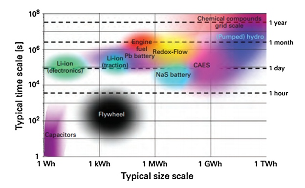
In this diagram, we see that such devices as capacitors store small amount of energy on the scale of seconds and minutes. At the same time, the systems shown in the right upper corner - pumped hydro storage, chemical storage - can store amounts of energy worth of gigawatt-hours over long periods of times (months to years). The same as with power generation technologies, storage system variety is important to satisfy various applications and demands and also to provide service storage in diverse natural and industrial settings.
The selection of the energy storage depends on many technical characteristics (besides scale), which would help us to understand why some technologies are preferred over others, and what trade-offs are involved in this selection. Let us look at some key storage characteristics next.
10.2 Key Metrics and Definitions for Energy Storage
Key Metrics and Definitions for Energy Storage
There are a few key technical parameters that are used to characterize a specific storage technology or system. Those characteristics will determine compatibility of the storage with a proposed application and will also have impact on its economic feasibility. Let us go through some definitions.
Storage Capacity
Capacity essentially means how much energy maximum you can store in the system. For example, if a battery is fully charged, how many watt-hours are put in there? If the water reservoir in the pumped hydro storage system is filled to capacity, how many watt-hours can be generated by releasing that water? Those amounts are determined by storage capacity.
Understandably, the capacity of any storage will increase with the system size. The more battery stacks are installed, the more electric energy can be put in for storage. The larger the water reservoir, the greater energy turnaround becomes possible. The system size should be matched with the load and specific application.
Storage capacity is typically measured in units of energy: kilowatt-hours (kWh), megawatt-hours (MWh), or megajoules (MJ). You will typically see capacities specified for a particular facility with storage or as total installed capacities within an area or a country.
| Portable scale | A portable battery pack with a storage capacity of 450 Wh... |
|---|---|
| Utility scale | One of the largest PV + storage projects in Texas – Upton 2 – has storage capacity of 42 MWh (which would be sufficient to power 1400 homes for 24 hours) |
| National scale | The total installed capacity of energy storage is the US is around 1000 MWh |
Sometimes you will see capacity of storage specified in units of power (watt and its multiples) and time (hours).
For example: 60 MW battery system with 4 hours of storage. What does it mean?
60 MW means that the system can generate electricity at the maximum power of 60 MW for 4 hours straight. That also means that the total amount of energy stored in the system is:
60 MW x 4 hours = 240 MWh
But it can also provide less power if needed. For example, if the load only requires 20 MW, the system can supply it for 12 hours. The total amount of stored energy is the same, but it is used more slowly:
20 MW x 12 hours = 240 MWh
So power and time ratings give us a little bit more information: we not only know how much energy is stored, but can also define at what maximum rate this energy can be potentially used.
Check Your Understanding Questions 1 & 2 (Multiple Choice)
Energy density
Energy density is often used to compare different energy storage technologies. This parameter relates the storage capacity to the size or the mass of the system, essentially showing how much energy (Wh) can be stored per unit cell, unit mass (kg), or unit volume (liter) of the material or device.
For example, energy densities for different types of batteries are listed in the table below [IES, 2011]:
| Battery type | Energy Density, Wh/liter |
|---|---|
| Lead-Acid battery | 50-80 |
| Li-ion battery | 200-400 |
| NiCd (nickel cadmium) battery | 15-80 |
| NiMH (nickel metal hydride) battery | 80-200 |
| NaS (sodium sulfur) battery | 150-300 |
| NaNiCl2 (sodium-nickel-chloride) battery | 150-200 |
| Zinc air battery | 130-200 |
| Vanadium redox flow battery | 20-70 |
| Hybrid flow battery | 65 |
Of course, we are interested to store as much energy as possible while using as small and light device as possible for this purpose. From the table above we can conclude, for example, that a fully charged Lead-Acid battery will run out of charge much sooner than a fully charged Li-ion battery of the same mass/size.
Energy density is related to capacity and determines the duration of power generation. Also materials with higher energy density help make the power block more compact, which is useful in portable electronics and vehicle applications.
Just for comparison, the energy density of the pumped hydro storage is 0.2—2 Wh/kg, which is rather low and requires significant masses of water and large reservoir size to deliver utility scale power.
Check Your Understanding Question 3 (Multiple Choice)
Power density
Power density (measured in W/kg or W/liter) indicates how quickly a particular storage system can release power. Storage devices with higher power density can power bigger loads and appliances without going oversize. Imagine an electric vehicle accelerating from 0 to 60 MPH – which takes a lot of power. If you look at the table below, you will see why Li-ion battery remains the technology of choice for powering electric vehicles, even though some other battery types exhibit similar energy densities.
| Battery type | Energy Density, Wh/liter | Power Density, W/liter |
|---|---|---|
| Lead-Acid battery | 50-80 | 90-700 |
| Li-ion battery | 200-400 | 1300-10000 |
| NiCd (nickel cadmium) battery | 15-80 | 75-700 |
| NiMH (nickel metal hydride) battery | 80-200 | 500-3000 |
| NaS (sodium sulfur) battery | 150-300 | 120-160 |
| NaNiCl2 (sodium-nickel-chloride) battery | 150-200 | 250-270 |
| Zinc air battery | 130-200 | 50-100 |
| Vanadium redox flow battery | 20-70 | .05-2 |
| Hybrid flow battery | 65 | 1-25 |
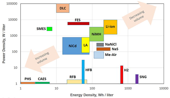
Key to abbreviations to Figure 10.2
CAES – Compressed Air Energy Storage
DLS – Double Layer Capacitor
FES – Flywheel Energy Storage
H2 – Hydrogen storage
LA – Lead Acid Battery
Li-ion – Li ion Battery
Me-air – Metal Air Battery
NaNiCl – Sodium Nickel Chloride Battery
NaS – Sodium Sulfur Battery
NiCd – Nickel Cadmium Vented Battery
NiMH – Nickel Metal Hydride Battery
PHS – Pumped Hydro Storage
RFB – Redox Flow Battery
SMES – Superconducting Magnetic Energy Storage
SNG – Synthetic Natural Gas
The technologies located in the lower left corner of the diagram (low energy density and low power density) take significant amount of space and material to enable the storage conversion and are mostly suitable for very large scale projects. Systems such as PHS and CAES also rely on the availability of specific landscape and geological features to accommodate the storage reservoirs.
The technologies located in the upper right corner of the diagram are most coveted for portable and efficient power supply, such as electric vehicles. These compact systems can carry a significant amount of energy and release it quickly on demand.
The technologies in the upper left corner are special devices that can be used in quick response electronics. These systems store small amounts of energy (and therefore charging can be fast), but are able to provide high power by releasing energy within short period of time.
Finally, the technologies in the lower right corner are characterized by slow charge and discharge, but the advantage is the total high amount of energy they are able to store, providing longer duration of energy supply.
Check Your Understanding Questions 4 & 5 (Multiple Choice)
Storage efficiency
The main function of any storage device is to uptake and release power on demand. In case of a battery, for example, it would be electrochemical charge/discharge cycle; in case of pumped hydro storage, this process involves pumping water into the elevated reservoir and later releasing the flow through the turbine. Both charge and discharge processes include one or more energy conversions (Figure 10.3). In the figure, each arrow indicates the energy conversion from one form to another.
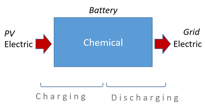
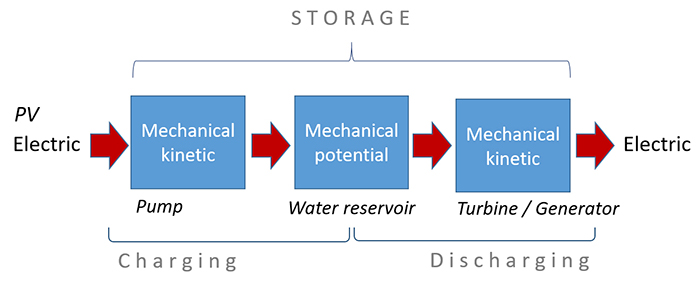
Regardless the number of transformations, the energy comes to its initial electric form, which is finally ready to be dispatched into the grid. This is the charge-discharge cycle, the "round trip".
In each conversion, energy is partially lost from the cycle and dissipated into the surroundings, and the efficiency of conversion at every step accounts for those losses.
Efficiencies of all energy conversion steps in this cycle are combined in the metric called round-trip efficiency, which essentially indicates the percentage of energy delivered by the storage system compared to the energy initially supplied to the storage system. The obvious goal is to minimize the conversion losses and thus maximize the overall storage efficiency.
Here are some round-trip efficiencies of various energy storage systems:
| Storage system | Round-trip efficiency, % |
|---|---|
| Lead-Acid battery | 75-90 |
| Li-ion battery | 85-98 |
| Pumped hydro storage | 70-80 |
| Compressed air energy storage | 41-75 |
| Flywheel | 80-90 |
| Hydrogen | 34-44 |
| Double layer capacitors | 85-98 |
| Vanadium redox flow battery | 60-75 |
These numbers mean the following. For example, out of 1 MWh of energy spent to pump water up to the hydro storage, only 0.7-0.8 MWh will be available to use after the water is released to run the turbine and generator to produce electric power. The other 0.2-0.3 MWh of energy will be converted into non-useful forms of energy and “lost” from the cycle. Some of the energy losses occur in the auxiliary devices used in the energy storage process, very often in the form of waste heat. Furthermore, energy losses may be linked to the mechanical or material losses: for example, leaks and evaporation of water from pumped storage, air leaks in CAES, chemical degradation and incomplete reactions in batteries.
Check Your Understanding Questions 6 & 7 (Multiple Choice)
10.3 Implementation of Utility Scale Storage - Battery Arrays
Implementation of Utility Scale Storage - Battery Arrays
The large-scale energy storage (also called grid energy storage) is a stand-alone or hybrid system that allows storing large amounts of electrical energy within an electrical power grid. Until recently, the dominant form of grid-scale energy storage has been pumped hydroelectricity, which accounts for over 95% of global installed storage capacity. Pumped hydro storage is rather old technology and has been around since the early 20th century, however it did not prove to be economically profitable or highly efficient. Other challenge you face in pumped hydro is the need of a certain kind of geological terrain to accommodate the proper size reservoir and availability of a large amount of water. We can add to that the environmental concerns and possible human impacts that are typically associated with the large hydro plants. It appears to be really hard to adopt this version of storage quickly in the newly constructed energy facilities.
Currently, there is a pressing need for new generation storage devices, that would be efficient, cheap, and possibly modular in order to facilitate their allocation at any location with any required capacity. This niche is currently being filled by the battery array systems. Battery arrays are often stand-alone facilities, strategically located to support regional grid stability.
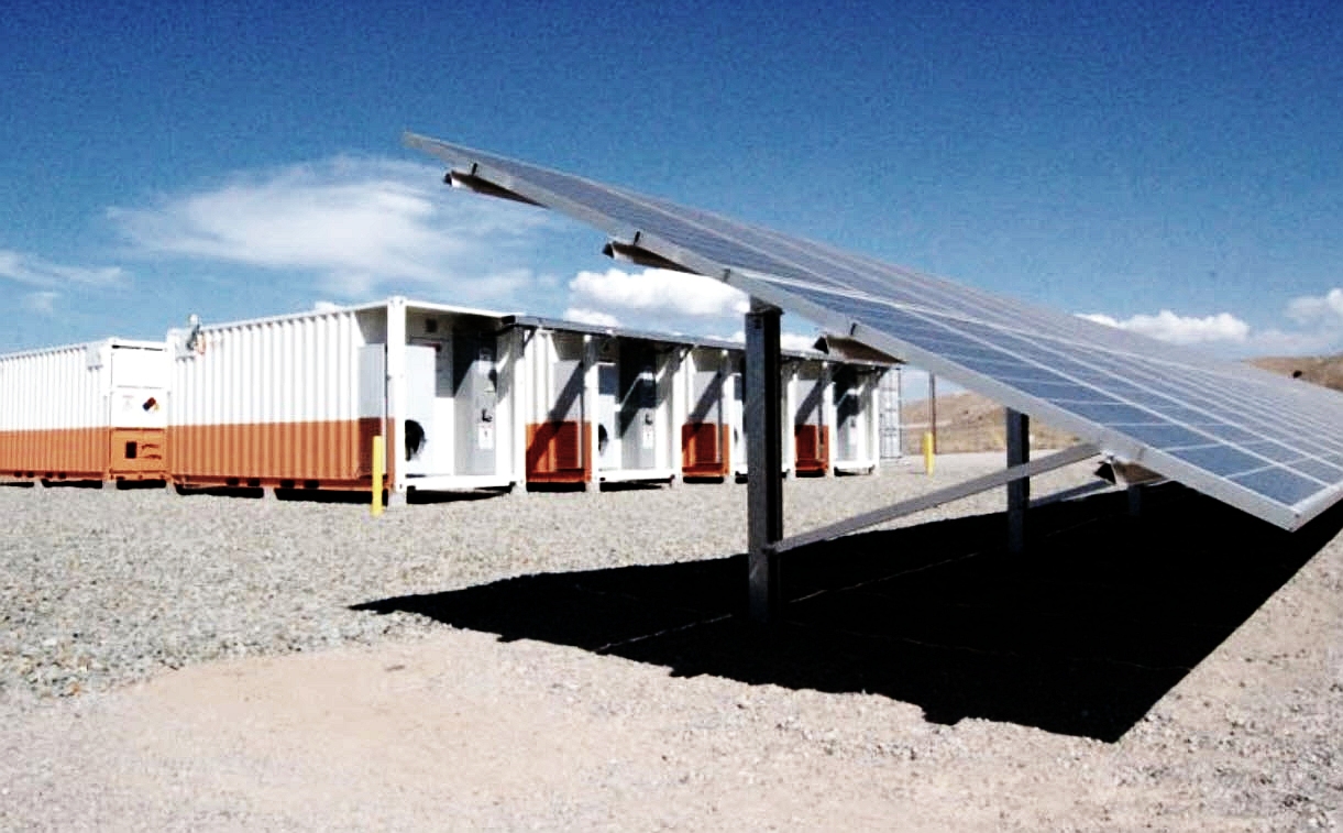
To be clear, the large battery energy storage systems (BESS) are not huge batteries as a matter of fact. Battery arrays are modulirized systems, in which individual battery cells (for example, Li-ion batteries) are stacked in series into higher voltage units. The same as solar cells are combined in panels, and pannels are organized in arrays, scaling-up battery systems follows the same principles of series and parallel connections in order to achieve the required power and capacity.
Some major companies that pursuing development and installation of large battery arrays are AES and Tesla. Follow the links below to learn about some case studies of battery array implementation:
- Tesla's Hornsdale Power Reserve in Australia:
- AES Case Studies of Stationary Storage:
- Angamos Storage Array
One of the advantages we can see with battery solutions for grid storage is flexibility. For one, they can act as a reliable backup source. In the event of a power outage, battery systems can be turned on quickly to compensate. Data shown in the presentation on Chile grid system (second link for Angamos Storage Array) demonstrate very quick response of the arrays to the power outage and successful grid balancing.
In Australia, Hornsdale Power Reserve (built byTesla) helped restore power to the country’s grid in a fraction of a second after an unexpected failure at a power plant.
"the Hornsdale Power Reserve has smoothed out at least two major energy outages, responding even more quickly than the coal-fired backups that were supposed to provide emergency power.
Tesla's battery last week kicked in just 0.14 seconds after one of Australia's biggest plants, the Loy Yang facility in the neighboring state of Victoria, suffered a sudden, unexplained drop in output, according to the International Business Times. And the week before that, another failure at Loy Yang prompted the Hornsdale battery to respond in as little as four seconds — or less, according to some estimates — beating other plants to the punch. State officials have called the response time “a record,” according to local media." (Washington Post, 2017 [139])
This table provides a list of other operating or commissioned projects, also including those based on other battery types (in addition to Li-ion):
| Project | Battery type | Location | Storage Capacity | Status/Date |
|---|---|---|---|---|
| Kingfisher Project | Lithium-ion | Roxby Downs, South Australia, Australia | 102 MW | Announced Dec 01, 2017 |
| AES Alamitos Energy Storage Array | Lithium-ion | Long Beach, CA, US | 100 MW | Contracted |
| Germany Residential Energy Storage Systems - 34,000 PV Battery Storage Systems@2 kW | Lithium-ion | Multiple, Multiple, Germany | 68 MW | Operational/Jan 31, 2016 |
| Kyushu Electric - Buzen Substation - Mitsubishi Electric/NGK Insulators | Sodium-sulfur | Buzen, Fukuoka Prefecture, Japan | 50 MW | Operational/Mar 03, 2016 |
| Gyeongsan Substation ESS - 48 MW ESS - KEPCO/Woojin/LG Chem | Lithium-ion | Gyeongsan-si, Gyeongsangbuk-do, Korea, South | 48 MW | Operational/Jul 01, 2016 |
| Nishi-Sendai Substation - Tohoku Electric/ Toshiba | Lithium-ion | Sendai, Miyagi Prefecture, Japan | 40 MW | Operational/Feb 20, 2015 |
| Minami-Soma Substation - Tohuka Electric/Toshiba | Lithium-ion | Minamisoma, Fukushima Prefecture, Japan | 40 MW | Operational/Feb 26, 2016 |
| 40 MW - AES/National Grid Corp. of the Philippines (Kabankalan) | Lithium-ion | Kabankalan, Negros, Occidental, Philippines | 40 MW | Operational |
| Notrees Battery Storage Project - Duke Energy | Advanced lead-acid | Goldsmith, TX, US | 36 MW | Operational/Jan 01, 2013 |
| Non-Gong Substation ESS - 36 MW ESS - KEPCO/Kokam | Lithium nickel manganese cobalt | Non-Gong Substation, N/A, Korea, South | 36 MW | Contracted |
| Rokkasho Village Wind Farm - Futamata Wind Development | Sodium-sulfur | Rokkasho, Aomori, Japan | 34 MW | Operational/May 01, 2008 |
| AES Laurel Mountain | Lithium-ion | Elkins, WV, US | 32 MW | Operational/Oct 01, 2011 |
| Beech Ridge Wind Storage | Lithium iron phosphate | Rupert, WV, US | 31.5 MW | Operational/Nov 04, 2015 |
| Grand Ridge Energy Storage | Lithium iron phosphate | Marseilles, IL, US | 31.5 MW | Operational/May 14, 2015 |
| Japan-Egypt-Hurghada | Lithium-ion | HurGhada, Red Sea Governorate, Egypt | 30 MW |
Announced |
| SDG&E Escondido Substation - AES | Lithium-ion | Escondido, CA, US | 30 MW | Contracted/Jan 31, 2017 |
| 30 MW SK Innovation BESS | Lithium-ion | Magdeberg, Saxony-Anhalt, Germany | 30 MW | Announced |
| Golden Hills - NextEra Energy | Lithium-ion | Livermore, CA, US | 30 MW | Contracted |
| Imperial Irrigation District BESS - GE | Lithium-ion | El Centro, CA, US | 30 MW | Under Construction/Oct 01, 2016 |
Source: Zhang, Wei, Cao, Lin. Energy storage system: Current studies on batteries and power condition system. [140] Renewable and Sustainable Energy Reviews. 2018 Feb; 82 (3): 3091-3106.
Batteries can also store extra energy. If there's excess power during peak wind or solar production, a battery can store up all that energy for future use. The Hornsdale plant is able to provide full power to 30,000 home, although for a relatively short period of time. In case of long outages, it still needs to be supported by traditional power generation facilities. In this way, battery essentially serves as an end user of power as well as a power plant.
According to National Renewable Energy Laboratory (NREL Report, 2018 [141]), the cost of the stand-alone utility scale Li-ion battery storage system breaks down as follows:
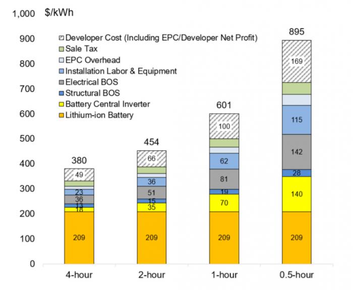
Interesting to note that while the battery cost per unit energy remains the same (with battery system being modular), the costs related to the balance of system, installation, and service decline with the storage duration.
PV + Storage Systems
Co-locating the PV and storage systems has multiple benefits. Co-location results in cost savings by reducing costs related to site preparation, land acquisition, permitting, interconnection, installation labor, hardware (via sharing of hardware such as switchgears, transformers, and controls), overhead, and profit. The cost of the co-located, DC-coupled system is 8% lower than the cost of the system with PV and storage sited separately, and the cost of the co-located, AC-coupled system is 7% lower. (NREL Report, 2018 [141])
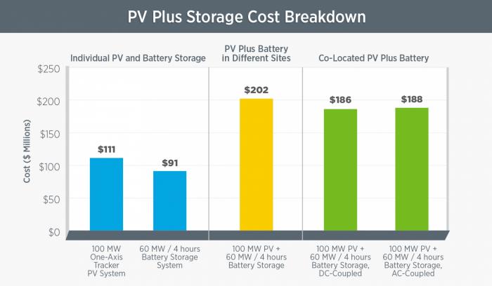
DC-coupling or AC-coupling of the energy source with storage can be used in different scenarios. DC-coupling is less expensive due to fewer conversions - 1% lower total cost than AC-coupling, which is the net result of cost differences between DC-coupling and AC-coupling in the categories of solar inverter, structural balance of system (BOS), electrical BOS, labor, EPC (engineering, procurement, and construction) and developer overhead, sales tax, contingency, and profit.
“According to NREL, there’s only one utility-scale PV system in the United States connected to storage, and it is Lawa'i project in Kauai, Hawaii. There are more systems that have storage co-located with a solar array, but those batteries can be charged by other sources of power on the grid. According to GTM Research’s “U.S. Energy Storage Monitor 2017 Year in Review,” more than 5,500 energy storage systems are installed in the U.S., in the residential and commercial sectors with over 95% connected to PV in the residential sector at the end of 2017, which amounts to about 4,700 systems. By the end of 2018, GTM estimates that solar-plus-storage will have accounted for about 4% of distributed PV and could reach 27% by 2023.” (Energy.gov, 2019 [142])
Based on this assessment, it looks like distributed PV market is somewhat ahead of the utility solar when it comes to hybrid PV+storage systems. It may change quickly. Look at the South Korea’s example:
“South Korea represents a story of how government planning can drive massive energy storage market growth, with a new policy to allow storage-backed wind and solar projects to earn renewable energy certificates worth five times their capacity value driving a massive boom in 2018. From less than 10 megawatt-hours deployed in 2017, South Korea’s utility-scale and commercial-industrial behind-the-meter deployments boomed to 1,100 megawatt-hours in 2018, with nearly $400 million in energy storage investments and a pipeline of projects that’s already overshot its goal of 800 megawatt-hours by 2020.” (JTM, 2019 [143])
But let us take a closer look at the Lawa'i Solar and Energy Storage plant on Kauai (HI), and try to find out what conditions made commission of this project a success.
Reading Assignment
Web article: Roselund, C., The Birth of the Solar+Storage Peaker [144], pv magazine, January 8, 2019.
This article gives you some basic information on the setting and parameters of the plant. But let us not stop there. The project was commissioned in the beginning of 2019. I ask you to research some more information on its current status and share your findings on the class discussion thread.
10.4 Resource Constraints and Environmental Considerations
Resource Constraints and Environmental Considerations
With energy storage industry changing fast, technology maturing, costs dropping, we can envision major shifts in both portable and stationary power markets. Cars and trucks will be powered by lithium-ion batteries rather than fossil fuel based internal combustion engines. Rechargeable lithium-ion batteries are also becoming crucial components of the new generation power grid to store increasing amounts of energy produced by solar and wind farms. This major technological scale-up will rely on the supply of new critical minerals and materials, such as lithium (Li), the lightest metal in the periodic table.
When thinking about this new future for our transportation and power industry, a few questions pop in our minds:
Where are we going to get all that lithium? (We are talking possibly 4-5 times topping the current market, perhaps more!) Is there enough of it on Earth? We are running out of oil, so would running out of lithium would get us in a similar trouble? How would prices for lithium affect international energy market and national economies of countries with higher or lower natural resource of this metal?
Companies such as Tesla, for example, already began a quest for control over lithium deposits across the globe, including countries in South America, Africa, and Australia.
Finally, mining and extraction of lithium at the accelerated rates will inevitably lead to serious environmental impacts on local and regional ecosystems (like any mining does), so how do these activities need to be regulated to keep this technology from becoming another global threat to biodiversity and human health?
To clarify some of these concerns, we are going to take a quick dive into the lithium lifecycle and learn about the key geological sources of its stock.
Reading Assignment
Web article: Gramling, C., The Search for New Geologic Sources of Lithium could Power a Clean Future [145], Science News, Vol. 195, No. 9, May 11, 2019, p. 40.
Mineral Spodumene is considered one of the key lithium ores and has been mined widely for multiple markets and applications.
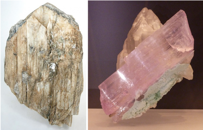
Prospecting for lithium and estimates of natural reserves have been done by U.S. Geological Survey at different years, and numbers keep changing due to discovering new deposits and, on the other hand, due to increasing demand for lithium from the energy storage and vehicle industry. For example in 2015, USGS estimated that world has lithium reserves for 365 years based on the global average production rate of 37,000 tons per year. Since then production has been doubled at least and the estimate shifted.
This is relatively recent (February 2019) USGS report, which provides some statistics on currently estimated reserves and production.
Reading Assignment
USGS Report: Mineral Commodity Summaries: Lithium, 2019 [148]
This information can be the starting point for assessing the available reserves for Li-ion battery manufacturing and forecasting Li markets.
Countries that contain the largest lithium reserves include Argentina, Chile, Australia, and China. Among them, Australia is currently the leader in mining and production. You can make your own calculations based on the data provided and compare to some other online reports (but I am sure this information is not set in stone).
Next, answer a few self-check questions based on the above readings.
Check Your Understanding Question 8 (Multiple Choice)
Check Your Understanding Question 9 (Essay)
What is currently the most economically viable source of naturally available lithium at the moment due to the cheapest method of extraction?
Check Your Understanding Question 10 (Multiple Choice)
On the other side of the equation, we also need to understand the options for lithium disposal and recycling in the end of the battery lifetime.
Environmental Risks
Production and disposal of Li-ion batteries are associated with an array of environmental and health impacts, which include soil and water pollution due to open-pit Li mining, bio-toxicity, aquatic ecotoxicity (impact on fish), release of carcinogenic substances, high water and energy use. These impacts are not only associated with Li metal itself, but also with chemicals used to extract it from rocks or brines.

Supplemental Reading:
Website: Check out this website for more information on Li mining [150] and extraction, methods, and major impacts in various regions of the World.
Recycling of components and materials contained in Li-ion batteries becomes of paramount importance to mitigate two major issues: (1) resource depletion and (2) environmental pollution. Effective recycling programs would help reduce the need for opening new Li mines and offset the rate of lithium resource exhaustion at the national and global scales. Recycling routes would also help divert the battery products from landfills and thus avoid risks associated with chemical dispersion in soils, streams, and aquifers.
That said, the Li-ion battery recycling industry is really at its infancy still:
- Currently recycling of EV batteries consists of storage, landfill, and/or pyrometallurgical processes (burning in smelters).
- China - Legislated that all EV manufacturers and importers come up with a feasible recycling program.
- European Union - Has set a timeline for battery manufactures and importers to recycle spent lithium ion batteries.
- Canada - Has three provinces (British Columbia, Manitoba and Quebec) with mandatory recycling programs.
- USA - There is no Federal Regulations for battery recycling, some States do have.
(Source: Seeking Alfa, 2018 [151])
For the next discussion assignment, we will try to search for signs of new business developments and regulations inside and outside of the U.S. related to Li-ion battery recycling and see how things have improved over the recent couple of years.
Summary and Activities
Summary and Activities
This lesson overviewed the main trends in the development of the large-scale energy storage systems. These systems are considered to be pivotal enabling technologies for greater penetration of renewables into the power grid. Cost, size, and ability to quickly install storage at any location on demand are key factors that will ensure the dispatchability of the new energy resources. Choosing the proper storage technology and sizing the system for a project can be a tricky balancing act between the ability to meet power requirements over a certain period of time and investment cost. In this lesson, you had a chance to study several successful operating solar+storage projects that provide us with a realistic picture of benefits as well as challenges of utility scale storage implementation.
Please go through the following activities to complete this lesson.
| Type | Description/Instructions | Deadline |
|---|---|---|
| Readings | Complete all necessary reading assigned in this lesson. | |
| Discussion Forum |
Solar + Storage Peaking Plant For this discussion, you will do some web research on Lawa'i Solar and Energy Storage Project installed by AES in Kauai (Hawaii). Based on your findings, you will share your thoughts on the motivation and specific prerequisites for this PV+BESS installation, as well as review the successes and challenges of this project. Further guidance for this assignment is provided in Module 10 in Canvas |
Sunday night |
| Activity |
PV + BESS Sizing Consider the following hypothetical scenario: Penn State’s main campus (University Park) aims to cover 25% of its electricity needs by solar energy. For that purpose, a utility scale PV + battery array system is to be deployed. The system should be able to provide 25% power off-grid if necessary. The PV plant will be feeding the load during the day and will also charge the BESS storage, which will be used to supply power during the night hours. Your goals will be (1) to determine the nameplate capacity for the PV installation and capacity of the BESS storage to meet the generation target, and (2) research vendors for BESS storage and suggest some options for storage units to deploy. Please see more specific instructions for this assignment in Module 10 in Canvas |
Wednesday night |
Individual Course Project
This last week of the semester is entirely reserved for the completion of your course project. The course project is a significant part of learning in this course, and it will be the way to apply the concepts learned to the evaluation of an existing solar energy facility. The project report should be built as a comprehensive review of multiple aspects and technologies involved in a utility-scale solar power generation.
For your project, you pick an existing solar plant, which may be a PV, CPV, or CSP facility operating in the U.S. or elsewhere. The main objective is to collect available information about this facility and to analyze different technological systems within it, including light concentration, tracking, energy conversion, power conditioning, operation parameters, etc. We spread out the research and writing tasks related to this project development through the semester, and the table below provides a list of the graded submissions.
| Timeline of course project development | What should be submitted | Due date | % of total grade |
|---|---|---|---|
| Selection of topic | Preliminary title of the project and one paragraph justification | Week 4 / See Canvas Calendar for due dates | 1% |
| Peer Review of project topics | Comments on peer submissions | Week 4 / See Canvas Calendar for due dates | 1% |
| Technology review | Written draft on technical background and status of technology involved in the facility (~4-5 pages) | Week 9 / See Canvas Calendar for due dates | 8% |
| Final report submission | Written final report summarizing your assessment | Week 12 / See Canvas Calendar for due dates | 30% |
Key components
This evaluation project should present the review of a number of important aspects that enable the power generation on the utility scale and are responsible for the process being technically feasible and economically viable. You may want to include the following sections, although this list is not exhaustive, and the content of the project may be build around the information you will be able to find:
- Topic, motivation, and goals
- Technology review
- Environmental setting and solar resource at the plant location
- System performance (analysis of existing data or modeling)
- Economic assessment
- Outlook and promise
You may plan additional sections in your report - anything you think would be important and relevant to your subject or to the specific socio-economic setting or location.
While this assessment is largely data compilation, and you will be using multiple sources to develop it, you need to critically evaluate the data and bring your own perspective to the discussion.
Tips on project submissions
Choice of a topic
Below are a couple of links that provide initial information on large-scale facilities, but you can find others, too.
If you think of choosing a particular plant, you may want to research it a little to see how much information is available. It would be preferable to have a variety of resources involved - government documents, published papers, web media, company releases. The more sources, the more comprehensive review you can build.
Technology review
These are some of the questions you may try to answer in this review:
- What technologies are involved in the design of the chosen solar facility, and what is their function?
- What technical principles are behind these technologies?
- How is deployment of these technologies justified at this particular locale?
- Are these technologies well-developed or new?
- What commercial vendors provide these technologies and associated equipment?
- What are alternatives and future perspectives in technological development of the plant?
Here, by technologies, we mean various technical components of the solar energy conversion. For example, in case of a photovoltaic plant, the key technologies to describe will be the type of PV cells used, module and array design, type of inverters, tracking systems, structural components (mounting frames etc.), energy storage system, monitoring and control systems, grid connection.
When describing these technologies, please refer to the specifics used at this particular plant. Provide images or graphics for better illustration. Originally prepared graphics is highly encouraged. If you borrow some images from the internet, please provide credits. List references to any sources you use, including websites. For proper way of citing references, please see CSE reference style.
Preparation of the Final Report
Your report should be an originally written document that summarizes your investigation of a chosen utility-scale solar facility. It should be comprehensive and deep enough research to qualify you as an analytical expert in key matters that provide for sustainable operation of this power plant.
The final report should include the previously prepared technology section, although feel free to expand and improve it, based on the instructor's feedback. Other sections should cover the above-mentioned required components and how they are implemented at this specific locale. If you are familiar with the System Advisor Model [153] (SAM) software, which is available for free from the National Renewable Energy Lab website, it would be appropriate to use it for analysis. The final report should also discuss the matters of component integration and issues related to large-scale power generation and connection to the grid. How are these matters currently handled by plant management? Specific applications and clients that use the power supplied by the plant should be mentioned. Any important aspects of social adaptation and policy related to the plant construction and operation in the area can also be included. List references to any sources you use, including websites. For the proper way of citing references, please see CSE reference style [154].
The following rubrics will be used in the evaluation of final projects:
- Depth of the technological background
- Coverage of the key issues
- Proper articulation and analysis of plant performance data
- Critical thinking and personal perspective
- Completeness of data search and references
- Structure, presentation, and graphics
Good luck completing your project reports and have a great end of the semester!