Chapter 2: Shrinking and Flattening the Globe: Scale, Projections, and Datums
Overview
Chapter 1 outlined several of the distinguishing properties of geographic information. One of these properties is that geographic maps are necessarily generalized, and that generalization tends to vary with scale. This chapter will introduce another distinguishing property related to the measurement and display of geographic information: that the Earth's complex, nearly-spherical but somewhat irregular shape complicates efforts to specify exact positions on the Earth's surface. In this chapter, we will explore the implications of these properties by illuminating concepts of scale, Earth geometry, coordinate systems, and the "horizontal datums" that define the relationship between coordinate systems and the Earth's shape.
Objectives
Compared to Chapter 1, Chapter 2 may seem long, technical, and abstract, particularly to those for whom these concepts are new. Chapter 2 will introduce some of the more technical concepts that are relevant to map construction and map reading. Students who successfully complete Chapter 2 will be able to:
- understand the concept of map scale and the multiple ways it is specified;
- demonstrate your ability to specify geographic locations using geographic coordinates;
- convert geographic coordinates between two different formats;
- explain the concept of a horizontal datum;
- recognize the kind of transformation that is appropriate to geo-register two or more data sets;
- describe the characteristics of the UTM coordinate system, including its basis in the Transverse Mercator map projection;
- describe the characteristics of the SPC system, including map projection on which it is based;
- interpret distortion diagrams to identify geometric properties of the sphere that are preserved by a particular map projection;
- classify projected map graticules by projection family.
Table of Contents:
- What is Scale?
- The Need for Coordinate Systems
- What are Map Projections?
- The Nearly Spherical Earth
- Glossary
- Biblography
Chapter lead adapter: Raechel Bianchetti.
Portions of this chapter were drawn directly from the following text:
Joshua Stevens, Jennifer M. Smith, and Raechel A. Bianchetti (2012), Mapping Our Changing World, Editors: Alan M. MacEachren and Donna J. Peuquet, University Park, PA: Department of Geography, The Pennsylvania State University.
2.1 What is Scale?
You hear the word "scale" often when you work around people who produce or use geographic information. If you listen closely, you will notice that the term has several different meanings, depending on the context in which it is used. You will hear talk about the scales of geographic phenomena and about the scales at which phenomena are represented on maps. You may even hear the word used as a verb, as in "scaling a map" or "downscaling." The goal of this section is for you to learn to tell these different meanings apart, and to be able to use concepts of scale to help make sense of geographic data.
2.1.1 Scope or Extent
Often "scale" is used as a synonym for "scope," or "extent." For example, the title of the article “Contractors Are Accused in Large-Scale Theft of Food Aid in Somalia,” [1] uses the term "large scale" to describe a widespread theft of food aid. This usage is common among the public. The term scale can also take on other meanings.
2.1.2 Measurement
The word "scale" can also be used as a synonym for a ruler--a measurement scale. Because data consist of symbols that represent measurements of phenomena, it is important to understand the reference systems used to take the measurements in the first place. In this section, we will consider a measurement scale known as the geographic coordinate system that is used to specify positions on the Earth's roughly spherical surface. In other sections, we will encounter two-dimensional (plane) coordinate systems, as well as the measurement scales used to specify attribute data.
2.1.3 Map Scale
Map scale is the proportion between a distance on a map and a corresponding distance on the ground (Dm / Dg). By convention, the proportion is expressed as a representative fraction in which map distance (Dm) is always reduced to 1. The representative fraction 1:100,000, for example, means that a section of road that measures 1 unit in length on a map stands for a section of road on the ground that is 100,000 units long. A representative fraction is unit-less, it has the same meaning if we are measuring on the map in inches, centimeters, or any other unit (in this example, the portion of the world represented on the map is 100,000 times as big as the map’s representation). If we were to change the scale of the map such that the length of the section of road on the map was reduced to, say, 0.1 units in length, we would have created a smaller-scale map whose representative fraction is 0.1:100,000, or 1:1,000,000.
2.1.4 Graphic Scales
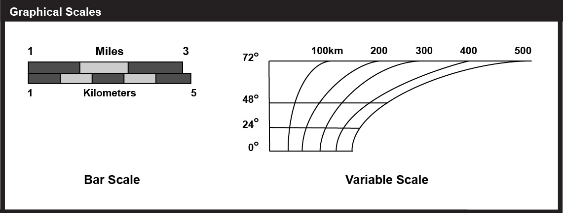
Another way to express map scale is with a graphic (or "bar") scale (Figure 2.1). Unlike representative fractions, graphic scales remain true when maps are shrunk or magnified, thus they are especially useful on web maps where it is impossible to predict the size at which users will view them. Most maps include a bar scale like the one shown above left. Some also express map scale as a representative fraction. The implication in either case is that scale is uniform across the map. However, except for maps that show only very small areas, scale varies across every map. This follows from the fact that positions on the nearly spherical Earth must be transformed to positions on two-dimensional sheets of paper. Systematic transformations of the world (or parts of it) to flat maps are called map projections. As we will discuss in greater depth later in this chapter, all map projections are accompanied by deformation of features in some or all areas of the map. This deformation causes map scale to vary across the map. Representative fractions typically, therefore, specify map scale along a line at which deformation is minimal (nominal scale). We will discuss nominal scale in further detail later. Bar scales, also, generally denote only the nominal or average map scale. An alternative to a simple bar scale that accounts for map distortion is a variable scale. Variable scales, like the one illustrated above right, show how scale varies, in this case by latitude, due to deformation caused by map projection.
2.1.5 Changing a Map's Size
As noted above, another way that the term "scale" is used is as a verb. To ‘scale a map’ is to reproduce it at a different size. For instance, if you photographically reduce a 1:100,000-scale map to 50 percent of its original width and height, the result would be one-quarter the area of the original. Obviously, the map scale of the reduction would be smaller too: 1/2 x 1/100,000 = 1/200,000 (or a representative fraction scale specification of 1:200,000). Because of the inaccuracies inherent in all geographic data, scrupulous geographic information specialists avoid enlarging source maps. To do so is to exaggerate generalizations and errors.
In the following sections, you will learn more about the process of converting the three-dimensional Earth into a two-dimensional visual representation, the map. As you move through the chapter, keep in mind the different meanings for the term "scale" and think about how it relates to the process of map creation.
Practice Quiz
Registered Penn State students should return now take the self-assessment quiz about the Map Scale.
You may take practice quizzes as many times as you wish. They are not scored and do not affect your grade in any way.
2.2 The Need for Coordinate Systems
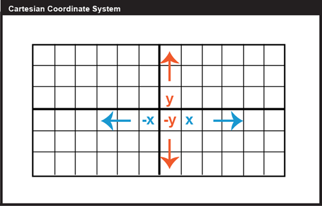
Locations on the Earth's surface are measured and represented in terms of coordinates; a coordinate is a set of two or more numbers that specifies the position of a point, line, or other geometric figure in relation to some reference system. The simplest system of this kind is a Cartesian coordinate system, named for the 17th century mathematician and philosopher René Descartes. A Cartesian coordinate system, like the one above in Figure 2.2, is simply a grid formed by put together two measurement scales, one horizontal (x) and one vertical (y). The point at which both x and y equal zero is called the origin of the coordinate system. In the illustration above, the origin (0,0) is located at the center of the grid (the intersection of the two bold lines). All other positions are specified relative to the origin. The coordinate of the upper right-hand corner of the grid is (6,3). The lower left-hand corner is (-6,-3).
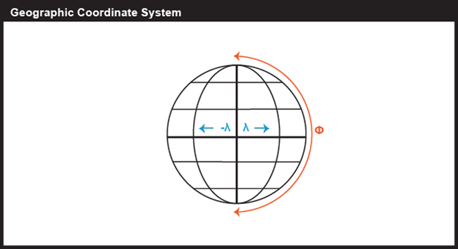
Cartesian and other two-dimensional (plane) coordinate systems are handy due to their simplicity. They are not perfectly suited to specifying geographic positions. However, the geographic coordinate system, as seen in Figure 2.3, is designed specifically to define positions on the Earth's roughly spherical surface. Instead of the two linear measurement scales x and y, the geographic coordinate systems bring together two curved measurement scales.
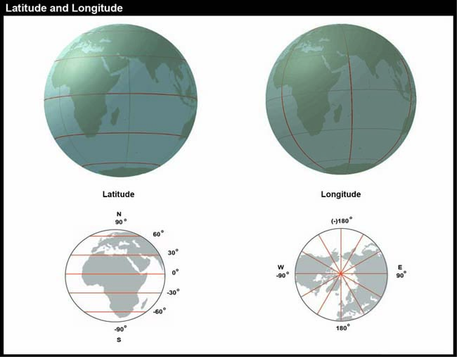
You have probably encountered the terms latitude and longitude before in your studies. A comparison of these two scales is given below in Figure 2.4. The north-south scale, called latitude (designated by the Greek symbol phi), ranges from +90° (or 90° N) at the North pole to -90° (or 90° S) at the South pole while the equator is 0°. A line of latitude is also known as a parallel.
The east-west scale, called longitude (conventionally designated by the Greek symbol lambda), ranges from +180° to -180°. Because the Earth is round, +180° (or 180° E) and -180° (or 180° W) are the same grid line. A line of longitude is called a meridian. That +/- 180 grid line is roughly the International Date Line, which has diversions that pass around some territories and island groups so that they do not need to cope with the confusion of nearby places being in two different days. Opposite the International Date Line on the other side of the globe is the prime meridian, the line of longitude defined by international treaty as 0°. At higher latitudes, the length of parallels decreases to zero at 90° North and South. Lines of longitude are not parallel, but converge toward the poles. Thus, while a degree of longitude at the equator is equal to a distance of about 111 kilometers, that distance decreases to zero at the poles.
Try This: Geographic Coordinate System Practice Application
Have you ever encountered the terms ‘latitude’ or ‘longitude’? How well do you understand the geographic coordinate system, really? Our experience is that while everyone who enters this class has heard of latitude and longitude, only about half can point to the location on a map that is specified by a pair of geographic coordinates. The websites linked below let you test your knowledge. You’ll practice by clicking locations on a globe as specified by randomly generated geographic coordinates.
Map Quiz Game [3]
2.2.1 Geographic Coordinates
We have discussed the fact that both latitude and longitude are measured in degrees, but what about when we need a finer granularity measurement? To record geographic coordinates, we can further divide degrees into minutes, and seconds. The degree is equal to sixty minutes, and each minute equal to sixty seconds. Geographic coordinates often need to be converted in order to geo-register one data layer onto another. Geographic coordinates may be expressed in decimal degrees, or in degrees, minutes, and seconds. Sometimes, you need to convert from one form to another.
Here's how it works:
To convert Latitude of -89.40062 from decimal degrees to degrees, minutes, seconds:
Subtract the number of whole degrees (89°) from the total (89.40062°). (The minus sign is used in the decimal degree format only to indicate that the value is a west longitude or a south latitude.) In this example, the minus sign indicates South, so keep track of that.
Multiply the remainder by 60 minutes (.40062 x 60 = 24.0372).
Subtract the number of whole minutes (24') from the product.
Multiply the remainder by 60 seconds (.0372 x 60 = 2.232). Round off (to the nearest second in this case).
Assemble the pieces; the result is 89° 24' 2" S. If the starting point had been the Longitude of -89.400062, the only difference would be that the S above would be replaced by a W.
To convert 43° 4' 31" from degrees, minutes, seconds to decimal degrees, use the simple formula below:
DD = Degrees + (Minutes/60) + (Seconds/3600)
Divide the number of seconds by 60 (31 ÷ 60 = 0.5166).
Add the quotient of step (1) to the whole number of minutes (4 + 0.5166).
Divide the result of step (2) by 60 (4.5166 ÷ 60 = 0.0753).
Add the quotient of step (3) to the number of whole number degrees (43 + 0.0753).
The result is 43.0753°
Practice Quiz
Registered Penn State students should return now take the self-assessment quiz about Geographic Coordinates.
You may take practice quizzes as many times as you wish. They are not scored and do not affect your grade in any way.
2.2.2 Plane Coordinates
So far, you have read about Cartesian Coordinate Systems, but that is not the only kind of 2D coordinate system. A plane coordinate system can be thought of as the juxtaposition of any two measurement scales. In other words, if you were to place two rulers at right angles, such that the "0" marks of the rulers aligned, you would define a plane coordinate system. The rulers are called "axes." Just as in Cartesian Coordinates, the absolute location of any point in the space in the plane coordinate system is defined in terms of distance measurements along the x (east-west) and y (north-south) axes. A position defined by the coordinates (1,1) is located one unit to the right, and one unit up from the origin (0,0). The Universal Transverse Mercator (UTM) grid is a widely-used type of geographic plane coordinate system in which positions are specified as eastings (distances, in meters, east of an origin) and northings (distances north of the origin).
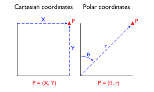
Some coordinate transformations are simple. The transformation from non-georeferenced plane coordinates to non-georeferenced polar coordinates, described in further detail later in the chapter, shown below involves nothing more than the replacement of one kind of coordinates with another.
2.2.3 UTM: Universal Transverse Mercator
The geographic coordinate system grid of latitudes and longitudes consists of two curved measurement scales to fit the nearly-spherical shape of the Earth. As discussed above, geographic coordinates can be specified in degrees, minutes, and seconds of arc. Curved grids are inconvenient to use for plotting positions on flat maps. Furthermore, calculating distances, directions, and areas with spherical coordinates is cumbersome in comparison to doing so with plane coordinates. For these reasons, cartographers and military officials in Europe and the U.S. developed the UTM coordinate system. UTM grids are now standard not only on printed topographic maps but also for the geographic referencing of the digital data that comprise the emerging U.S. "National Map" (NationalMap.gov [8]).
"Transverse Mercator" refers to the manner in which geographic coordinates are transformed from a spherical model of the Earth into plane coordinates. The act of mathematically transforming geographic spherical coordinates to plane coordinates necessarily displaces most (but not all) of the transformed coordinates to some extent. Because of this, map scale varies within projected (plane) UTM coordinate system grids. Thus, UTM coordinates provide locations specifications that are precise, but have known amounts of positional error depending on where the place is.
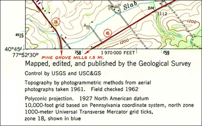
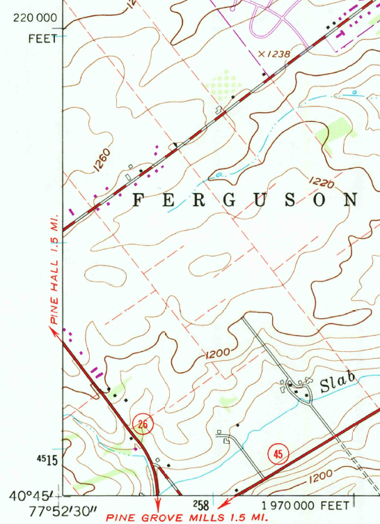
Shown below is the southwest corner of a 1:24,000-scale (for which 1 inch on the map represents 2000 ft. in the world) State College topographic map in Centre County, PA, published by the United States Geological Survey (USGS). Note that the geographic coordinates (40° 45' N latitude, 77° 52' 30" W longitude) of the corner are specified. Also shown, however, are ticks and labels representing two plane coordinate systems, the Universal Transverse Mercator (UTM) system and the State Plane Coordinates (SPC) system. The tick on the west edge of the map labeled "4515" represents a UTM grid line (called a "northing") that runs parallel to, and 4,515,000 meters north of, the equator. Ticks labeled "258" and "259" represent grid lines that run perpendicular to the equator and 258,000 meters and 259,000 meters east, respectively, of the origin of the UTM Zone 18 North grid (see its location on Fig 6 above). Unlike longitude lines, UTM "eastings" are straight and do not converge upon the Earth's poles.
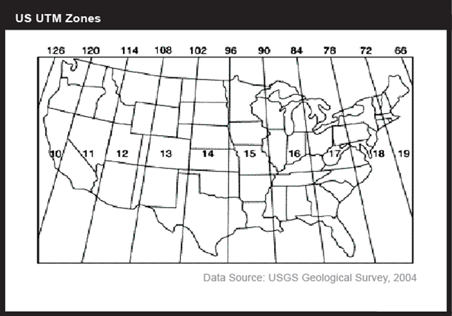
The Universal Transverse Mercator system is not really universal, but it does cover nearly the entire Earth surface. Only polar areas--latitudes higher than 84° North and 80° South--are excluded. (Polar coordinate systems are used to specify positions beyond these latitudes.) The UTM system divides the remainder of the Earth's surface into 60 zones, each spanning 6° of longitude. These are numbered west to east from 1 to 60, starting at 180° West longitude (roughly coincident with the International Date Line).
The illustration above depicts UTM zones as if they were uniformly "wide" from the Equator to their northern and southern limits. In fact, since meridians converge toward the poles on the globe, every UTM zone tapers from 666,000 meters in "width" at the Equator (where 1° of longitude is about 111 kilometers in length) to only about 70,000 meters at 84° North and about 116,000 meters at 80° South.
To clarify this, the illustration below depicts the area covered by a single UTM coordinate system grid zone. Each UTM zone spans 6° of longitude, from 84° North to 80° South. Each UTM zone is subdivided along the equator into two halves, north and south.
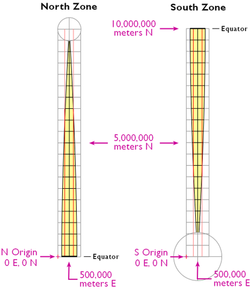
The illustration above shows how UTM coordinate grids relate to the area of coverage illustrated above. The north and south halves are shown side by side for comparison. Each half is assigned its own origin. The north south zone origins are positioned to south and west of the zone. North zone origins are positioned on the Equator, 500,000 meters west of the central meridian for that zone. Origins are positioned so that every coordinate value within every zone is a positive number. This minimizes the chance of errors in distance and area calculations. By definition, both origins are located 500,000 meters west of the central meridian of the zone (in other words, the easting of the central meridian is always 500,000 meters E). These are considered "false" origins since they are located outside the zones to which they refer. UTM eastings specifying places within the zone range from 167,000 meters to 833,000 meters at the equator. These ranges narrow toward the poles. Northings range from 0 meters to nearly 9,400,000 in North zones and from just over 1,000,000 meters to 10,000,000 meters in South zones. Note that positions at latitudes higher than 84° North and 80° South are defined in Polar Stereographic coordinate systems that supplement the UTM system.
The distorted ellipse graph below shows the amount of distortion on a UTM map. This kind of plot will be explained in more detail below; the key thing to note here is that the size and shape of features plotted in red indicate the amount of size and shape distortion across the map (a wide range in sizes indicates substantial area distortion, a range from circles to flat ellipses indicates substantial shape distortion). The ellipses centered within the highlighted UTM zone are all the same size and shape. Away from the highlighted zone, the ellipses steadily increase in size, although their shapes remain uniformly circular. This pattern indicates that scale distortion is minimal within Zone 30, and that map scale increases away from that zone. Furthermore, the ellipses reveal that the character of distortion associated with this projection is that shapes of features as they appear on a globe are preserved while their relative sizes are distorted. Map projections that preserve shape by sacrificing the fidelity of sizes are called conformal projections. The plane coordinate systems used most widely in the U.S., UTM and SPC (the State Plane Coordinates system), are both based upon conformal projections.
The Transverse Mercator projection illustrated above minimizes distortion within UTM zone 30 by putting that zone at the center of the projection. Fifty-nine variations on this projection are used to minimize distortion in the other 59 UTM zones. In every case, distortion is no greater than 1 part in 1,000. This means that a 1,000 meter distance measured anywhere within a UTM zone will be no worse than + or - 1 meter off.
One disadvantage of the UTM system is that multiple coordinate systems must be used to account for large entities. The lower 48 United States, for instance, spreads across ten UTM zones. The fact that there are many narrow UTM zones can lead to confusion. For example, the city of Philadelphia, Pennsylvania is east of the city of Pittsburgh. If you compare the Eastings of centroids representing the two cities, however, Philadelphia's Easting (about 486,000 meters) is less than Pittsburgh's (about 586,000 meters). Why? Because although the cities are both located in the U.S. state of Pennsylvania, they are situated in two different UTM zones. As it happens, Philadelphia is closer to the origin of its Zone 18 than Pittsburgh is to the origin of its Zone 17. If you were to plot the points representing the two cities on a map, ignoring the fact that the two zones are two distinct coordinate systems, Philadelphia would appear to the west of Pittsburgh. Inexperienced GIS users make this mistake all the time. Fortunately, GIS software is getting sophisticated enough to recognize and merge different coordinate systems automatically.
Practice Quiz
Registered Penn State students should return now take the self-assessment quiz about the UTM Coordinates.
You may take practice quizzes as many times as you wish. They are not scored and do not affect your grade in any way.
2.2.4 State Plane Coordinates
The UTM system was designed to meet the need for plane coordinates to specify geographic locations globally. Focusing on just the U.S., in consultation with various state agencies, the U.S. National Geodetic Survey (NGS) devised the State Plane Coordinate System with several design objectives in mind. Chief among these were:
- plane coordinates for ease of use in calculations of distances and areas;
- all positive values to minimize calculation errors; and
- a maximum error rate of 1 part in 10,000.
As discussed above, plane coordinates specify positions in flat grids. Map projections are needed to transform latitude and longitude coordinates to plane coordinates. The designers of the SPCS did two things to minimize the inevitable distortion associated with projecting the Earth onto a flat surface. First, they divided the U.S. into 124 relatively small zones that cover the 50 U.S. states. Second, they used slightly different map projection formulae for each zone, one that minimizes distortion along either the east-west or north-south line depending on the orientation of the zone. The curved, dashed red lines in the illustration below represent the two standard lines that pass through each zone. Standard lines indicate where a map projection has zero area or shape distortion (some projections have only one standard line).
As shown below, some states are covered with a single zone while others are divided into multiple zones. Each zone is based upon a unique map projection that minimizes distortion in that zone to 1 part in 10,000 or better. In other words, a distance measurement of 10,000 meters will be at worst one meter off (not including instrument error, human error, etc.). The error rate varies across each zone, from zero along the projection's standard lines to the maximum at points farthest from the standard lines. Errors will be much lower than the maximum at most locations within a given SPC zone. SPC zones achieve better accuracy than UTM zones because they cover smaller areas, and so are less susceptible to projection-related distortion.
As we have seen above, positions in any coordinate system are specified relative to an origin. Like UTM zones, SPC zone origins are defined so as to ensure that every easting and northing in every zone are positive numbers. As shown in the illustration below, SPC origins are positioned south of the counties included in each zone. The origins coincide with the central meridian of the map projection upon which each zone is based. The false origin of the Pennsylvania North zone, is defined as 600,000 meters East, 0 meters North. Origin eastings vary from zone to zone from 200,000 to 8,000,000 meters East.
The SPCS zones are identified with a 4 digita FIPS code, the first two digits represents the state and the second the zone (e.g., PA has a FIPS code of 37 with 2 zones, 1 and 2, thus 3701 for the nothern zone and 3702 for the sourthern). The starting "0" for states in the 1-9 range is typically dropped; thus for CA, as an example, the most norther SPCS zone is 401.
One place you can look up all zone numbers is here: USA State Plane Zones NAD83 [10]
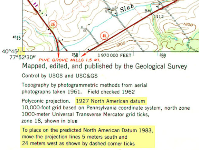
Shown below is the southwest corner of the same 1:24,000-scale topographic map used as an example above. Along with the geographic coordinates (40 45' N latitude, 77° 52' 30" W longitude) of the corner and UTM tick marks discussed above, SPCS eastings and northings are also included. The tick labeled "1 970 000 FEET" represents a SPC grid line that runs perpendicular to the equator and 1,970,000 feet east of the origin of the Pennsylvania North zone. Notice that, in this example, SPC system coordinates are specified in feet rather than meters. The SPC system switched to use of meters in 1983, but most existing topographic maps are older than that and still give the specification in feet (as in the example below). The origin lies far to the west of this map sheet. Other SPC grid lines, called "northings" (the one for 220,000 FEET is shown), run parallel to the equator and perpendicular to SPC eastings at increments of 10,000 feet. Unlike longitude lines, SPC eastings and northings are straight and do not converge upon the Earth's poles.
SPCs, like all plane coordinate systems, pretend the world is flat. The basic design problem that confronted the geodesists who designed the State Plane Coordinate System was to establish coordinate system zones that were small enough to minimize distortion to an acceptable level, but large enough to be useful.
Most SPC zones are based on either a Transverse Mercator or Lambert Conic Conformal map projection whose parameters (such as standard line(s) and central meridians) are optimized for each particular zone. "Tall" zones like those in New York state, Illinois, and Idaho are based upon unique Transverse Mercator projections that minimize distortion by running two standard lines north-south on either side of the central meridian of each zone, much as the same projection is used for UTM zones. "Wide" zones like those in Pennsylvania, Kansas, and California are based on unique Lambert Conformal Conic projections (see below for more on this and other projections) that run two standard lines (standard parallels, in this case) west-east through each zone. (One of Alaska's zones is based upon an "oblique" variant of the Mercator projection. That means that instead of standard lines parallel to a central meridian, as in the transverse case, the Oblique Mercator runs two standard lines that are tilted so as to minimize distortion along the Alaskan panhandle.)
These two types of map projections share the property of conformality, which means that angles plotted in the coordinate system are equal to angles measured on the surface of the Earth. As you can imagine, conformality is a useful property for land surveyors, who make their livings measuring angles.
This section has hinted at some of the characteristics of map projections and how they are used to relate plane coordinates to the globe. Next, we delve more deeply into the topic of map projections, a topic that has fascinated many mathematicians and others over centuries.
Practice Quiz
Registered Penn State students should return now take the self-assessment quiz about the State Plane Coordinates.
You may take practice quizzes as many times as you wish. They are not scored and do not affect your grade in any way.
2.3 What are Map Projections?
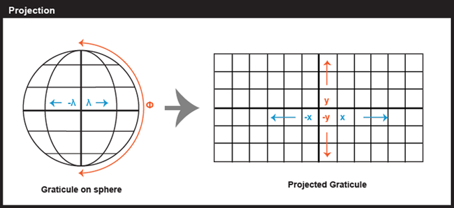
Latitude and longitude coordinates specify positions in a spherical grid called the graticule (that approximates the more-or-less spherical Earth). The true geographic coordinates called unprojected coordinate in contrast to plane coordinates, like the Universal Transverse Mercator (UTM) and State Plane Coordinates (SPC) systems, that denote positions in flattened grids. These georeferenced plane coordinates are referred to as projected. The mathematical equations used to project latitude and longitude coordinates to plane coordinates are called map projections. Inverse projection formulae transform plane coordinates to geographic. The simplest kind of projection, illustrated below, transforms the graticule into a rectangular grid in which all grid lines are straight, intersect at right angles, and are equally spaced. Projections that are more complex yield grids in which the lengths, shapes, and spacing of the grid lines vary. Even this simplest projection produces various kinds of distortions; thus, it is necessary to have multiple types of projections to avoid specific types of distortions. Imagine the kinds of distortion that would be needed if you sliced open a soccer ball and tried to force it to be completely flat and rectangular with no overlapping sections. That is the amount of distortion we have in the simple projection below (one of the more common in web maps of the world today).
Many types of map projections have been devised to suit particular purposes. The term "projection" implies that the ball-shaped net of parallels and meridians is transformed by casting its shadow upon some flat, or flattenable, surface. While almost all map projection methods are created using mathematical equations, the analogy of an optical projection onto a flattenable surface is useful as a means to classify the bewildering variety of projection equations devised over the past two thousand years or more.
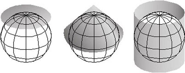
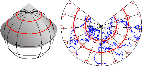
There are three main categories of map projection, those in which projection is directly onto a flat plane, those onto a cone sitting on the sphere that can be unwrapped, and other onto a cylinder around the sphere that can be unrolled (Figure 2.15 above). All three are shown in their normal aspects. The plane often is centered upon a pole. The cone is typically aligned with the globe such that its line of contact (tangency) coincides with a parallel in the mid-latitudes. Moreover, the cylinder is frequently positioned tangent to the equator (unless it is rotated 90°, as it is in the Transverse Mercator projection). As you might imagine, the appearance of the projected grid will change quite a lot depending on the type of surface it is projected onto, how that surface is aligned with the globe, and where that imagined light is held. The following illustrations show some of the projected graticules produced by projection equations in each category.
- Cylindric projection equations yield projected graticules with straight meridians and parallels that intersect at right angles. The example shown above is a Cylindrical Equidistant (also called Plate Carrée or geographic) in its normal equatorial aspect.
- Pseudocylindric projections are variants on cylindrics in which meridians are curved. The result of a Sinusoidal projection is shown above.
- Conic projections yield straight meridians that converge toward a single point at the poles, parallels that form concentric arcs. The example shown above is the result of an Albers Conic Equal Area, which is frequently used for thematic mapping of mid-latitude regions.
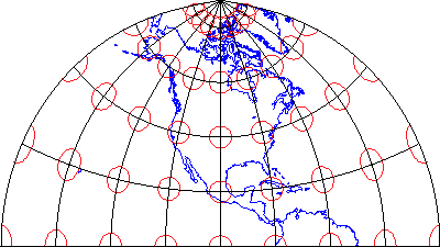
- Planar projections also yield meridians that are straight and convergent, but parallels form concentric circles rather than arcs. Planar projections are also called azimuthal because every planar projection preserves the property of azimuthality, directions (azimuths) from one or two points to all other points on the map. The projected graticule shown above is the result of an Azimuthal Equidistant projection in its normal polar aspect.
Appearances can be deceiving. It is important to remember that the look of a projected graticule depends on several projection parameters, including latitude of projection origin, central meridian, standard line(s), and others. Customized map projections may look entirely different from the archetypes described above (Figure 2.16).
To help interpret the wide variety of projections, it is necessary to become familiar with Spatial Reference Information that traditionally accompanies a map. There are several terms that you must understand to read the Spatial Reference Information. First, the projection name identifies which projection was used. With this information, you get an understanding of the projection category and the geometric properties the projection preserves. Next, the central meridian is the location of the central longitude meridian. The Latitude of Projection defines the origin of latitude for the projection. There are three common aspects that we can define: polar (projections centered on a pole), equatorial (usually cylindrical or pseudo-cylindrical projections aligned with the equator), and oblique (those centered on any other place). Scale Factor at Central Meridian is the ratio of map scale along the central meridian and the scale at a standard meridian, where scale distortion is zero. Finally, some projections, including the Lambert Conic Conformal, include parameters by which you can specify one or two standard lines along which there is no scale distortion.
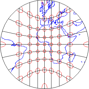
2.3.1 Map Projections: Distortion
No projection allows us to flatten the globe without distorting it. Distortion ellipses help us to visualize what type of distortion a map projection has caused, how much distortion occurred, and where it occurred. The ellipses show how imaginary circles on the globe are deformed because of a particular projection. If no distortion had occurred in the process of projecting the map shown below, all of the ellipses would be the same size, and circular in shape.
When positions on the graticule are transformed to positions on a projected grid, four types of distortion can occur: distortion of sizes, angles, distances, and directions. Map projections that avoid one or more of these types of distortion are said to preserve certain properties of the globe: equivalence, conformality, equidistance, and azimuthality, respectively. Each is described below.
2.3.1.1 Equivalence
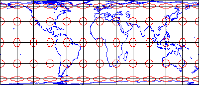
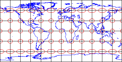
So-called equal-area projections maintain correct proportions in the sizes of areas on the globe and corresponding areas on the projected grid (allowing for differences in scale, of course). Notice that the shapes of the ellipses in the Cylindrical Equal Area projection above are distorted, but the areas each one occupies are equivalent. Equal-area projections are preferred for small-scale thematic mapping (discussed in the next chapter), especially when map viewers are expected to compare sizes of area features like countries and continents.
2.3.1.2 Conformality
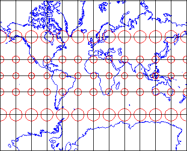
The distortion ellipses plotted on the conformal projection shown above vary substantially in size, but are all the same circular shape. The consistent shapes indicate that conformal projections preserve the fidelity of angle measurements from the globe to the plane. In other words, an angle measured by a land surveyor anywhere on the Earth's surface can be plotted at its corresponding location on a conformal projection without distortion. This useful property accounts for the fact that conformal projections are almost always used as the basis for large scale surveying and mapping. Among the most widely used conformal projections are the Transverse Mercator, Lambert Conformal Conic, and Polar Stereographic.
Conformality and equivalence are mutually exclusive properties. Whereas equal-area projections distort shapes while preserving fidelity of sizes, conformal projections distort sizes in the process of preserving shapes.
As discussed above in section 2.2.4, SPC zones that trend west to east (including Pennsylvania's) are based on unique Lambert Conformal Conic projections. Instead of the cylindrical projection surface used by projections like the Mercator shown above, the Lambert Conformal Conic and map projections like it employ conical projection surfaces like the one shown below. Notice the two lines at which the globe and the cone intersect. Both of these are standard lines; specifically, standard parallels. The latitudes of the standard parallels selected for each SPC zones minimize scale distortion throughout that zone.
2.3.1.3 Equidistance
Equidistant map projections allow distances to be measured accurately along straight lines radiating from one or, at most, two points or they can have correct distance (thus maintain scale) along one or more lines. In the example below (also sometimes called an "equirectangular" projection because the parallels and meridians are both equally spaced). Notice that ellipses plotted on the Cylindrical Equidistant (Plate Carrée) projection shown above vary in both shape and size. The north-south axis of every ellipse is the same length, however. This shows that distances are true-to-scale along every meridian; in other words, the property of equidistance on this map projection is preserved from the two poles.
2.3.1.4 Azimuthality
Azimuthal projections preserve directions (azimuths) from one or two points to all other points on the map. Gnomonic projections, like the one above, display all great circles as straight lines. A great circle is the most direct path between two locations across the surface of the globe. See how the ellipses plotted on the gnomonic projection shown above vary in both size and shape, but are all oriented toward the center of the projection. In this example, that is the one point at which directions measured on the globe are not distorted on the projected graticule. This is a good projection for uses like plotting airline connections from one airport to all others.
2.3.1.5 Compromise
Some map projections preserve none of the properties described above, but instead seek a compromise that minimizes distortion of all kinds. The example shown above is the Polyconic projection, where parallels are all non-concentric circular arcs, except for a straight equator, and the centers of these circles lie along a central axis. The U.S. Geological Survey used the polyconic projection for many years as the basis of its topographic quadrangle map series until the conformal Transverse Mercator succeeded it. Another example is the Robinson projection, which is often used for small-scale thematic maps of the world (it was used as the primary world map projection by the National Geographic Society from 1988-1997, then replaced with another compromise projection, the Winkel Tripel; thus, the latter has become common in textbooks).
Try This: Album of Map Projections
John Snyder and Phil Voxland (1994) published an Album of Map Projections that describes and illustrates many more examples in each projection category. Excerpts from that important work are included in our Interactive Album of Map Projections, which registered students will use to complete Project 1. The Interactive Album is available at the PSU Interactive Album of Map Projections [11].Flex Projector is a free, open source software program developed in Java that supports many more projections and variable parameters than the Interactive Album. Bernhard Jenny of the Institute of Cartography at ETH Zurich created the program with assistance from Tom Patterson of the US National Park Service. You can download Flex Projector from FlexProjector.com [12]
Those who wish to explore map projections in greater depth than is possible in this course might wish to visit an informative page published by the International Institute for Geo-Information Science and Earth Observation (Netherlands), which is known by the legacy acronym ITC. The page is available at Kartoweb Map Projections. [13]
Practice Quiz
Registered Penn State students should return now take the self-assessment quiz about the Map Projections.
You may take practice quizzes as many times as you wish. They are not scored and do not affect your grade in any way.
2.4 The Nearly Spherical Earth
You know that the Earth is not flat; but, as we have implied already, it is not spherical either! For many purposes, we can ignore the variation from a sphere; but, if accuracy matters, the Earth is best described as a geoid. A geoid is the equipotential surface of the Earth's gravity field; put simply, it has the shape of a lumpy, slightly squashed ball. Determining the precise shape of the geoid is a major concern of the science of geodesy, the study of Earth’s size, shape, and gravitational and magnetic fields. The accuracy of coordinates that specify geographic locations depends upon how the coordinate system grid is aligned with the Earth's surface, and that alignment depends on the model we use to represent the actual shape of the geoid. While geodesy is an old science, many challenging problems remain, and geodesists continue to make advances that increase our ability to locate places accurately (and that gradually make the location of the GPS in your phone more accurate).
Geoids are lumpy because gravity varies from place to place in response to local differences in terrain and variations in the density of materials in the Earth's interior. The Earth’s geoid is also a little squat, as suggested above. Sea level gravity at the poles is greater than sea level gravity at the equator, a consequence of Earth's "oblate" shape as well as the centrifugal force associated with its rotation.
Geodesists at the U.S. National Geodetic Survey (NGS Geoid 12A [14]) describe the geoid as an "equipotential surface" because the potential energy associated with the Earth's gravitational pull is equivalent everywhere on the surface. The geoid is essentially a three-dimensional mathematical surface that fits (as closely as possible) gravity measurements taken at millions of locations around the world. As additional, and more accurate, gravity measurements become available, geodesists revise the shape of the geoid periodically. Some geoid models are solved only for limited areas; GEOID03, for instance, is calculated only for the continental U.S.
It is important to differentiate the bumpiness of a geoid from the ruggedness of Earth’s terrain, since geoids depend on gravitational measurements and are not simply representations of Earth’s topographic features. Although Earth’s topography, which consists of extreme heights like Mount Everest (29,029 ft above sea level) and incredible depths like the Mariana Trench (36,069 ft below sea level), the Earth’s average terrain is relatively smooth. Astronomer Neil de Grasse Tyson (2009) points out: "Earth, as a cosmic object is remarkably smooth; if you had a giant finger and rubbed it across Earth's surface (oceans and all), Earth would feel as smooth as a cue ball. Expensive globes that portray raised portions of Earth’s landmasses to indicate mountain ranges depict a grossly exaggerated reality (p. 39)."
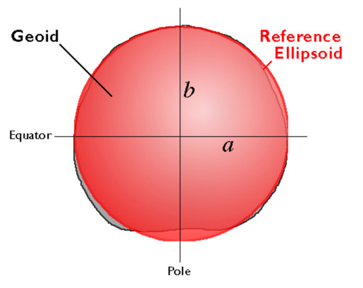
2.4.1 Ellipsoid
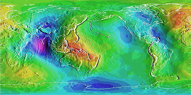
An ellipsoid is a three-dimensional geometric figure that resembles a sphere, but whose equatorial axis (a in the Figure 2.23 above) is slightly longer than its polar axis (b). Ellipsoids are commonly used as surrogates for geoids to simplify the mathematics involved in relating a coordinate system grid with a model of the Earth's shape. Ellipsoids are good, but not perfect, approximations of geoids; they more closely model the actual shape of the Earth than a simple sphere. One implication of different models of the Earth is that they represent elevation of places as different. Surveyors and engineers measure elevations at construction sites and elsewhere. Elevations are expressed in relation to a vertical datum, a reference surface such as mean sea level. Different geoids and different ellipsoids define the vertical datum differently. The map below (Figure 2.24) shows differences in elevation between the GEOID96 geoid model and the WGS84 ellipsoid. The surface of GEOID96 represents the surface as being 75 meters higher than does the WGS84 ellipsoid over New Guinea (where the map is colored red). In the Indian Ocean (where the map is colored purple), the surface of GEOID96 represents the surface as about 104 meters below the ellipsoid surface.
Many ellipsoids are in use around the world. Local ellipsoids minimize differences between the geoid and the ellipsoid for individual countries or continents. The Clarke 1866 ellipsoid, for example, minimizes deviations in North America.
Once we have identified a preferable shape with which to represent the Earth (the specific ellipsoid), the next consideration that we must make is the coordinate system to provide a means to define positions of locations on that sphere (spherical coordinate system).
2.4.2 Horizontal Datums
Horizontal datum is an elusive concept for many GIS practitioners. However, it is relatively easy to understand if we start with the concept that the datum defines the position of a coordinate system in relation to the places being located. Before considering horizontal datums in the context of geographic (spherical) coordinates, consider the simple example below that uses plane coordinates. In this example, the “datum” is a simple Cartesian grid. The figure shows what would happen if the horizontal datum of any plane coordinate system had a different origin from which all coordinates were determined (e.g., if the false origin of any SPCS zone was a slightly different place.
Starting from the above model, it is relatively easy to visualize a horizontal datum in the context of unprojected geographic coordinates in relation to a reference ellipsoid. Simply drape the latitude and longitude grid over the ellipsoid and shift it to align the coordinates with the ellipsoid appropriately, and there is your horizontal datum. It is harder to think about datum in the context of a projected coordinate grid like UTM and SPC, however. Think of it this way: First, drape the latitude and longitude grid on an ellipsoid. Then, project that grid to a 2-D plane surface. Finally, superimpose a rectangular grid of eastings and northings over the projection, using control points to geo-register the grids. There you have it--a projected coordinate grid based upon a horizontal datum. It would appear just like the example above; the difference is how we figure out the alignment between the grid and the world.
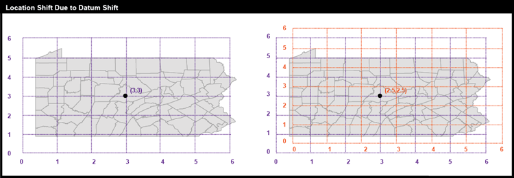
Around the world, geodesists define different horizontal datums that are appropriate (accurate) for different places. Datums are periodically updated as technology allows for increases in accuracy, but changes are infrequent since every time a change is made, there are serious implications (in cost and time) to update the position information for every place that the datum applies to. In the U.S., the two most frequently encountered horizontal datums are the North American Datum of 1927 (NAD 27) and the North American Datum of 1983 (NAD 83). The advent of the Global Positioning System (GPS) necessitated an update of NAD 27 to NAD 83 that included (a) adoption of a geocentric ellipsoid, GRS 80, in place of the Clarke 1866 ellipsoid; and (b) correction of many distortions that had accumulated in the older datum. Bearing in mind that the realization of a datum is a network of fixed control point locations that have been specified in relation to the same reference surface, the 1983 adjustment of the North American Datum caused the coordinate values of every control point managed by the National Geodetic Survey (NGS) to change. Obviously, the points themselves did not shift because of the datum transformation (although they did move a centimeter or more a year due to plate tectonics). Rather, the coordinate system grids based upon the datum shifted in relation to the new ellipsoid (just like the shift in plane coordinates illustrated above), and because local distortions were adjusted at the same time, the magnitude of grid shift varies from place to place. The illustration below compares the magnitude of the grid shifts associated with the NAD 83 adjustment at one location.
Given the irregularity of the shift (much more complex than the simple translation of the plane coordinate system shown in Figure 2.25), NGS could not suggest a simple transformation algorithm that surveyors and mappers could use to adjust local data based upon the older datum. Instead, NGS created a software program called NADCON (Dewhurst 1990, Mulcare 2004) that calculates adjusted coordinates from user-specified input coordinates by interpolation from a pair of 15° correction grids generated by NGS from hundreds of thousands of previously adjusted control points. The U.S. National Geodetic Survey (NGS Geoid Home [16]) maintains a database of the coordinate specifications of these control points, including historical locations as well as adjustments that are more recent.
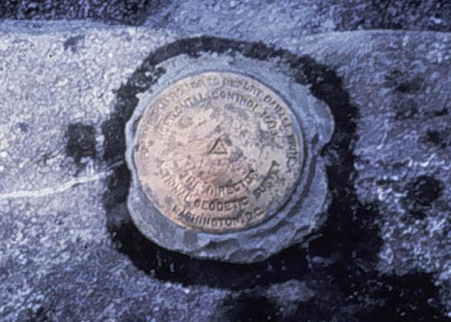
Geoids, ellipsoids, and even coordinate systems are all abstractions. The fact that a "horizontal datum" refers to a relationship between an ellipsoid and a coordinate system, two abstractions, may explain why the concept is so frequently misunderstood. Datums do have physical manifestations: approximately two million horizontal and vertical control points that have been established in the U.S. Although control point markers are fixed, the coordinates that specify their locations are liable to change. In the U.S., high-order horizontal control point locations are marked with permanent metal "monuments" like the one shown above in Figure 2.27. The physical manifestation of the datum is a network of control point measurements that are marked in the real world with these monuments (National Geodetic Survey, 2004).
Practice Quiz
Registered Penn State students should return now take the self-assessment quiz about The Nearly Spherical Earth.
You may take practice quizzes as many times as you wish. They are not scored and do not affect your grade in any way.
2.5 Glossary
Azimuthal Projection: A map projection that preserves directions (azimuths) from one or two points to all other points on the map.
Cartesian Coordinate System: A coordinate grid formed by putting together two measurement scales, one horizontal (x) and one vertical (y).
Conformal Projection: A map projection that preserve shape by sacrificing the fidelity of sizes.
Conic Projection: A map projection that yields straight meridians that converge toward a single point at the poles; parallels that form concentric arcs.
Coordinates: A set of two or more numbers specifying the position of a point, line, or other geometric figure in relation to some reference system.
Cylindric Projection: A map projection where projected graticules are straight meridians and parallels that intersect at right angles.
Decimal Degrees: The expression of geographic coordinates in the decimal form (i.e., 43.0753°).
Degrees, Minutes, and Seconds: The expression of geographic coordinates by degree, minute, and second values (i.e., 89° 24' 2" S).
Distortion Ellipse: A tool to visualize what type of distortion a map projection has caused, how much distortion occurred, and where it occurred.
Ellipsoid: A three-dimensional geometric figure that resembles a sphere, but whose equatorial axis (a) is slightly longer than its polar axis (b).
Equal-Area Projection: A map projection maintaining correct proportions in the sizes of areas on the globe and corresponding areas on the projected grid (allowing for differences in scale).
Equator: The equator is the 0-degree line of latitude.
Equidistant Projection: A map projection that allows distances to be measured accurately along straight lines radiating from one or two points only.
Geodesy: Geodesy is the scientific study of Earth’s size, shape, and gravitational and magnetic fields.
Geographic Coordinate System: The coordinate system that is used to specify positions on the Earth's roughly spherical surface.
Geoid: The equipotential surface of the Earth's gravity field; put simply, it has the shape of a lumpy, slightly squashed ball.
Gnomonic Projection: A map projection displaying all great circles as straight lines.
Graphic Scales: A visual tool for representing map scale; unlike representative fractions, graphic scales remain true when maps are shrunk or magnified.
Graticule: The graticule is the geographic coordinate system’s grid.
Great Circle: The most direct path between two locations across the surface of the globe.
Horizontal Datum: An abstraction which defines the relationship between coordinate systems and the Earth's shape.
International Date Line: Roughly the +/- 180 line of longitude.
Lambert Conic Conformal: A map projection whose parameters (such as standard line(s) and central meridians) are optimized for each particular zone.
Latitude: The east-west scale of the geographic coordinate system.
Longitude: The north-south scale of the geographic coordinate system.
Map Projections: Systematic transformations of the world (or parts of it) to flat maps .
Map Scale: The proportion between a distance on a map and a corresponding distance on the ground (Dm / Dg).
Meridian: A line of longitude.
Nominal Scale: A map scale line at which deformation is minimal.
Origin: The point at which both x and y equal zero.
Parallel: A line of latitude.
Planar Projection: Map projection (also called azimuthal projection) that yields meridians that are straight and convergent, and parallels form concentric circles.
Plane Coordinate System: A coordinate system defining a location on the Earth using x and y coordinates.
Prime Meridian: The line of longitude defined by international treaty as 0°.
Project: A method of representing the surface of a sphere or other three-dimensional body on a plane.
Pseudocylindric Projection: A variation of cylindric projection in which meridians are curved.
Representative Fraction: Proportion between a distance on a map and a corresponding distance on the ground (Dm / Dg) in which map distance (Dm) is always reduced to 1 and is unit-less.
Scale a Map: to reproduce a map at a different size.
Scale Factor at Central Meridian: the ratio of map scale along the central meridian and the scale at a standard meridian, where scale distortion is zero.
Standard Lines: A line specified in spatial reference information of a projection along which there is no scale distortion.
State Plane Coordinates: (SPCs) A plane coordinate system consisting of a set of 124 geographic zones or coordinate systems [17] designed for specific regions of the United States.
Transverse Mercator: A map projection that is an adaptation of the standard Mercator projection.
Unit-less: A value that has no units attached, it has the same meaning if we are measuring on the map in inches, centimeters, or any other unit.
Universal Transverse Mercator Coordinate System (UTM): A coordinate system which divides the remainder of the Earth's surface into 60 zones, each spanning 6° of longitude.
Unprojected: Coordinates which have not yet been projected to 2-D surface.
Variable Scale: A graphic representation of scale that shows variability of scale across a map.
Vertical Datum: A reference surface, such as mean sea level.
2.6 Bibliography
3-D Software (2005). Map projections pages [18]. Retrieved January 8, 2005, from www.3dsoftware.com
American Congress on Surveying and Mapping (n. d.). The North American Datum of 1983. A collection of papers describing the planning and implementation of the readjustment of the North American horizontal network. Monograph No. 2.
Burkard, R. K. et al. (1959-2002). Geodesy for the layman [19]. Retrieved October 29, 2003, from the National Imagery and Mapping Agency website: www.ngs.noaa.gov
Chem-Nuclear Systems, Inc. (1993). Site screening interim report: Stage two -- regional disqualification.Harrisburg PA.
Chrisman, N. (2002). Exploring geographic information systems (2nd ed.). New York: John Wiley & Sons.
Clarke, K. (1995). Analytical and computer cartography (2nd ed.). Upper Saddle River, NJ: Prentice Hall.
Dana, P. H. (1998). Coordinate systems overview. The Geographer's Craft Project [20]. Retrieved June 25, 2004, from The University of Colorado at Boulder, Department of Geography website: geography.colorado.edu [21]
Dana, P. H. (1999). Geodetic datums overview. The Geographer's Craft Project [20]. Retrieved June 25, 2004, from The University of Colorado at Bolder, Department of Geography website: geography.colorado.edu [21]
Dewhurst, W. T. (1990). NADCON: The application of minimum-curvature-derived surfaces in the transformation of positional data from the North American datum of 1927 to the North American datum of 1983. [22] NOAA Technical Memorandum NOS NGS 50. Retrieved January 1, 2005, from www.ngs.noaa.gov/PUBS_LIB/NGS50.pdf
Doyle, D. (2004, February). NGS geodetic toolkit, Part 7: Computing state plane coordinates. Professional Surveyor Magazine, 24:, 34-36.
Dutch, S. (2003). The Universal Transverse Mercator System [23]. Retrieved January 9, 2008, from www.uwgb.edu/DutchS/FieldMethods/UTMSystem.htm
Federal Geographic Data Committee. (December 2001). United States National Grid. Retrieved May 8, 2006, fromfgdc.gov/standards/projects/FGDC-standards-projects/usng/fgdc_std_011_2001_usng.pdf
Hildebrand, B. (1997). Waypoint+. Retrieved January 1, 2005, from www.tapr.org [24]
Iliffe, J.C. (2000). Datums and map projections for remote sensing, GIS and surveying. Caithness, Scotland: Whittles Publishing. Distributed in U.S. by CRC Press.
John P. Snyder (1993) Flattening the Earth: Two Thousand Years of Map Projections, University of Chicago Press, Chicago, IL
Larrimore, C. (2002). NGS Geodetic Toolkit [25]. Retrieved October 26, 2004, from noaa.gov/TOOLS
Muehrcke, P. C. & Muehrcke, J. O. (1992). Map use (3rd ed.). Madison WI: JP Publications.
Muehrcke, P. C. & Muehrcke, J. O. (1998). Map use (4th ed.). Madison WI: JP Publications.
Mulcare, D. M. (2004). The National Geodetic Survey NADCON Tool. Professional Surveyor Magazine, February, pp. 28-33.
National Geodetic Survey. (1997). Image generated from 15'x15' geoid undulations covering the planet Earth [26]. Retrieved 1999, from www.ngs.noaa.gov/GEOID [27]
National Geodetic Survey. (2004). Coast and geodetic survey historical image collection [26]. Retrieved June 25, 2004,https://photolib.noaa.gov/ [28]
National Geodetic Survey. (n.d.). North American datum conversion utility [26]. Retrieved April 2004, from www.ngs.noaa.gov/TOOLS/Nadcon/Nadcon.html
National Geographic Society (1999). Round Earth, flat maps [29]. Retrieved April 18, 2006, from www.nationalgeographic.com
Ordnance Survey (2000). National GPS network information. 7: Transverse mercator map projections. [30] Retrieved August 27, 2004, from www.gps.gov.uk/guide7.asp [31]
Robinson, A. et al. (1995). Elements of cartography (5th ed.). New York: John Wiley & Sons.
Robinson, A. H. & Snyder, J. P. (1997). ://courseware.e-education.psu.edu/projection/">Matching the map projection to the need [32]. Retrieved January 8, 2005, from the Cartography and Geographic Information Society and the Pennsylvania State University website: https://courseware.e-education.psu.edu/projection/
Slocum, T. A., McMaster, R. B., Kessler, F, C., & Howard, H. H. (2005). Thematic cartography and visualization (2nd ed.). Upper Saddle River, NJ: Prentice Hall.
Smith, J.R. (1988). Basic geodesy. Rancho Cordova CA: Landmark Enterprises.
Snyder, J. P. & Voxland P. M. (1989). An album of map projections (U.S. Geological Survey Professional Paper No. 1453). Washington DC: United States Government Printing Office.
Snyder, J. P. & Voxland, P. M. (1994). An album of map projections. (USGS Professional Paper No. 1453). Washington DC: U.S. Geological Survey. (ordering information published at USGS Publications Warehouse [33])
Snyder, J. P. (1987). Map projections: A working manual (U.S. Geological Survey Professional Paper No. 1395). Washington DC: United States Government Printing Office.
Snyder, J. P. (1987). Map projections: A working manual. (USGS Professional Paper No. 1395). Washington DC: U.S. Geological Survey.
Stem, J. E. (1990). State Plane Coordinate System of 1983 (NOAA Manual NOS NGS 5). Rockville, MD: National Geodetic Information Center.
Tyson, Neil deGrasse (2009). The Pluto Files: the Rise and Fall of America’s Favorite Planet. New York: W. W. Norton.
United States Geological Survey (2001). The universal transverse mercator grid [34]. Fact sheet 077-01. Retrieved June 30, 2004, from mac.usgs.gov (since retired).
United States Geological Survey (2003). National mapping program standards [35]. Retrieved October 29, 2005, from rockyweb.cr.usgs.gov/nmpstds/nmas647.html
USGS. "State College Quadrangle" [map]. 7.5 minute series. Washington, D.C.: USGS, 1962.
Van Sickle, J. (2004). Basic GIS coordinates. Boca Raton FL: CRC Press.
Wikipedia. The free encyclopedia. (2006). World geodetic system [36]. Retrieved May 8, 2006, from wikipedia.org/wiki/WGS84
Wolf, P. R. & Brinker, R. C. (1994) Elementary Surveying (9th ed.). New York NY: HarperCollins.
Slocum, T., Yoder, S., Kessler, F. and Sluter, R. 2000: MapTime: Software for Exploring Spatiotemporal Data Associated with Point Locations [37]. Cartographica: The International Journal for Geographic Information and Geovisualization 37, 15-32. dx.doi.org/10.3138/T91X-1N21-5336-2R73