Chapter 4: Encoding Our World: Geographic Data Representation
Overview
Information is a fundamental commodity, as discussed in Chapter 1, that it has become difficult or impossible for government agencies, businesses, other organizations, as well as individuals, to do without. Many of the problems and opportunities faced by organizations of all types are so complex, and involve so many locations, that the organizations need assistance in creating useful and timely information. That's what information systems are for. Information systems are computer-based tools that help people transform data into information.
Suppose that you've launched a new business that manufactures solar-powered lawn mowers. You're planning a mail campaign to bring this revolutionary new product to the attention of prospective buyers. But, since it's a small business, you can't afford to sponsor coast-to-coast television commercials, or to send brochures by mail to more than 100 million U.S. households. Instead, you plan to target the most likely customers - those who are environmentally conscious, have higher than average family incomes, and who live in areas where there is enough water and sunshine to support lawns and solar power.
Fortunately, lots of data are available to help you define your mailing list. Household incomes are routinely reported to banks and other financial institutions when families apply for mortgages, loans, and credit cards. Personal tastes related to issues like the environment are reflected in behaviors such as magazine subscriptions and credit card purchases. Firms like Claritas [1] collect such data and transform it into information by creating "lifestyle segments" - categories of households that have similar incomes and tastes. Your solar lawnmower company can purchase lifestyle segment information by 5-digit ZIP code, or even by ZIP+4 codes, which designate individual households.
It's astonishing how companies like Claritas can create valuable information from the millions upon millions of transactions that are recorded every day. Their products are made possible by the fact that the original data exist in digital form and because the companies have developed information systems that enable them to transform the data into information that companies like yours value. The fact that lifestyle information products are often delivered by geographic areas, such as ZIP codes, speaks to the appeal of geographic information systems (GIS). The scale of these data and their potential applications are increasing continually with the advent of new mechanisms for sharing information and making purchases that are linked to our GPS-enabled smartphones (more on those in Chapter 5). Here, we focus on how all the geographically-referenced data is organized, stored, and accessed in systems that turn the data into information.
A Geographical Information System (GIS) is a computer-based tool used to help people transform geographic data into geographic information.
The definition implies that a GIS is somehow different from other information systems, and that geographic data are different from non-geographic data. Let's consider these differences.
GIS arose out of the need to perform spatial queries on geographic data (questions addressed to a database such as wanting to know a distance or the location where two objects intersect). A spatial query requires knowledge of locations as well as attributes about that location. For example, an environmental analyst might want to know which public drinking water sources are located within one mile of a known toxic chemical spill. Or, a planner might be called upon to identify property parcels located in areas that are subject to flooding. To accommodate geographic data and spatial queries and help users understand the answer to their queries, the system for managing your data (i.e., a database management system) needs to be integrated with a mapping system. Until about 1990, most maps were printed from handmade drawings or engravings or at least had multiple manual processing steps between data collection and map generation. Geographic data produced by draftspersons consisted of graphic marks inscribed on paper or film. To this day, most of the lines that appear on topographic maps published by the U.S. Geological Survey were originally engraved by hand. The place names shown on the maps were affixed with tweezers, one word at a time. Needless to say, such maps were expensive to create and to keep up to date. Computerization of the mapmaking process had obvious appeal.
As stated earlier, information systems assist decision makers by enabling them to transform data into useful information. GIS specializes in helping users transform geographic data into geographic information. In particular, GIS enables decision makers to identify locations or routes whose attributes match multiple criteria, even though entities and attributes may be encoded in many different data files. A geographic information system uses a data model to incorporate geographic features from the real world into digital data representations. The geographic data are stored in a database and later displayed on a map. Users commonly manipulate and create new data within a database in order to solve a problem. For instance, a city planner may want to enhance public transportation by adding new bus lines. One important issue for the planner is to make sure new bus lines serve a large population. If the planner already has a geographic database with information on population and area for every city block, population density can be computed (density = population/area) into the existing database (Table 4.1).
| Block | Population | Area in Sq. Meters | Population Density |
|---|---|---|---|
| Block 1 | 97 | 1350 | 97/1350 =.07 |
| Block 2 | 254 | 410 | .61 |
| Block 3 | 296 | 275 | 1.08 |
| Block 4 | 122 | 450 | .27 |
| Block 5 | 158 | 700 | .03 |
| ... | ... | ... | ... |
Example of a portion of a table stored in a geographical database. This fictional table depicts data by Census Block (a geographical unit discussed in Chapter 3). In this database, this table will be dynamically linked to another that has coordinate information to define where the Census blocks referred to are in the world.
Credit: Jennifer M. Smith, Department of Geography, The Pennsylvania State University.
The hypothetical database above reveals that for Block 3, there are on average 1.08 people per square meter. Based on the database computations, the city planner should make the bus line stop on along Block 3 where the most people are located per square meter.
This chapter will explore the characteristics of digital data and how it is represented in a GIS by discussing how it is stored, managed, and manipulated.
Objectives
Students who successfully complete Chapter 4 should be able to:
- distinguish the difference between features and attributes;
- identify the different attribute measurement scales and basic operations for each type;
- understand what a database management system is and identify what it is used for;
- understand what metadata is and why it is used;
- identify the difference between vector and raster data.
Table of Contents
- Feature Versus Attributes
- Attribute Measurement Scales
- Database Managmenet Systems
- Metadata
- Vector Versus Raster
- Summary
- Glossary
- Biblography
Chapter lead author: Jennifer M. Smith.
Portions of this chapter were drawn directly from the following text:
Joshua Stevens, Jennifer M. Smith, and Raechel A. Bianchetti (2012), Mapping Our Changing World, Editors: Alan M. MacEachren and Donna J. Peuquet, University Park, PA: Department of Geography, The Pennsylvania State University.
4.1 Feature Versus Attributes
As discussed in Chapter One, geographic data represent spatial locations (i.e., a feature) and non-spatial attributes measured at certain times. For instance, a city (a feature with a spatial location) can contain an endless number of attributes. Geographic data for a specific city may include attributes such as its population, the types of public transportation, and various land use patterns. Over recent years, software developers have created variations on standard query languages (SQL) that incorporate spatial queries. The dynamic nature of geographic phenomena complicates the issue further, however. The need to pose spatio-temporal queries challenges geographic information scientists (GIScientists) to develop ever more sophisticated ways to represent geographic phenomena, thereby enabling analysts to interrogate their data in more sophisticated ways.
4.1.1 Tables: Location versus Attribute
To explore the differences between a location and its attributes, view the table below of a geographic database originating from the U.S. Census Bureau and imported into ESRI’s ArcMap program. Each row in the attribute table refers to a feature’s location on the map, with numerous attributes associated with it. In this example, each object refers to a state that includes attribute data including information such as its FID (unique identifier), shape (polygon), state abbreviation, full state name, a FIPS code (unique code assigned to each state), and the longitude and latitude coordinates. As you can see, the fifth row highlighted in light blue is selected and the mapping program automatically links to the spatial representation of the state of California, also outlined in light blue. This functionality allows users to manipulate, query, and select features and their attributes in the table, while viewing changes dynamically on the map.

4.2 Attribute Measurement Scales
Chapter 2 focused upon measurement scales for spatial data, including map scale (expressed as a representative fraction), coordinate grids, and map projections (methods for transforming three dimensional to two dimensional measurement scales). You may know that the meter, the length standard established for the international metric system, was originally defined as one-ten-millionth of the distance from the equator to the North Pole. In virtually every country except the United States, the metric system has benefited science and commerce by replacing fractions with decimals, and by introducing an Earth-based standard of measurement.
Standardized scales are needed to measure non-spatial attributes as well as spatial features. Unlike positions and distances, however, attributes of locations on the Earth's surface are often not amenable to absolute measurement. In a 1946 article in Science, a psychologist named S. S. Stevens outlined a system of four levels of measurement meant to enable social scientists to systematically measure and analyze phenomena that cannot simply be counted. (In 1997, geographer Nicholas Chrisman pointed out that a total of nine levels of measurement are needed to account for the variety of geographic data.) The levels are important to specialists in geographic information because they provide guidance about the proper use of different statistical, analytical, and cartographic operations. In the following, we consider examples of Stevens' original four levels of measurement: nominal, ordinal, interval, and ratio.
4.2.1 Nominal Level
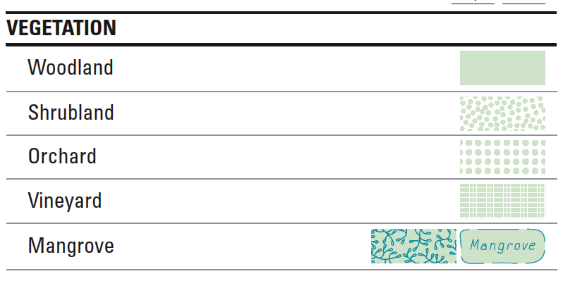
The term nominal simply means to relate to the word “name.” Simply put, nominal level data are data that are denoted with different names (e.g., forest, water, cultivated, wetlands), or categories. Data produced by assigning observations into unranked categories are nominal level measurements. In relation to terminology used in Chapter 1, nominal data are a type of categorical (qualitative) data. Specifically, nominal level data can be differentiated and grouped into categories by “kind,” but are not ranked from high to low. For example, one can classify the land cover at a certain location as woods, scrub, orchard, vineyard, or mangrove. There is no implication in this distinction, however, that a location classified as "woods" is twice as vegetated as another location classified "scrub."
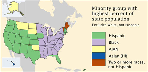
Although census data originate as individual counts, much of what is counted is individuals' membership in nominal categories. Race, ethnicity, marital status, mode of transportation to work (car, bus, subway, railroad...), and type of heating fuel (gas, fuel oil, coal, electricity...) are measured as numbers of observations assigned to unranked categories. For example, the map below, which appears in the Census Bureau's first atlas of the 2000 census, highlights the minority groups with the largest percentage of population in each U.S. state. Colors were chosen to differentiate the groups through a qualitative color scheme to show differences between the classes, but not to imply any quantitative ordering. Thus, although numerical data were used to determine which category each state is in, the map depicts the resulting nominal categories rather than the underlying numerical data.
4.2.2 Ordinal Level
Like the nominal level of measurement, ordinal scaling assigns observations to discrete categories. Ordinal categories, however, are ranked, or ordered – as the name implies. It was stated in the preceding section that nominal categories such as "woods" and "mangrove" do not take precedence over one another, unless a set of priorities is imposed upon them. This act of prioritizing nominal categories transforms nominal level measurements to the ordinal level. Because the categories are not based upon a numerical value (just an indication of an order or importance), ordinal data are also considered to be categorical (or qualitative).
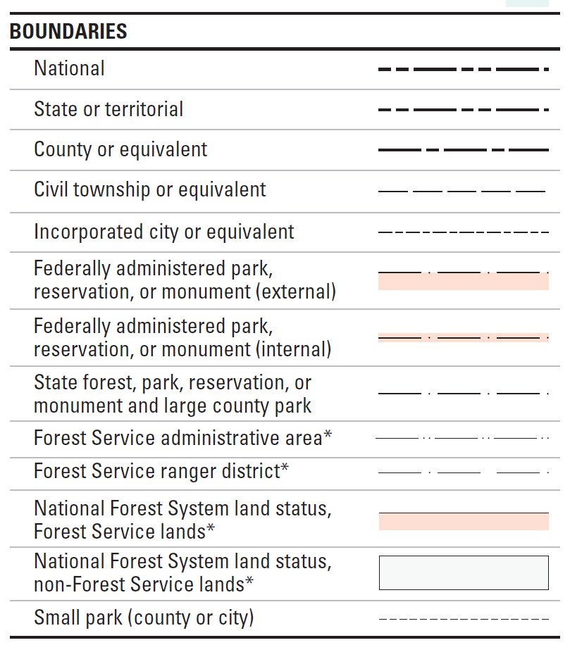
Examples of ordinal data often seen on reference maps include political boundaries that are classified hierarchically (national, state, county, etc.) and transportation routes (primary highway, secondary highway, light-duty road, unimproved road). Ordinal data measured by the Census Bureau include how well individuals speak English (very well, well, not well, not at all), and level of educational attainment (high school graduate, some college no degree, etc.). Social surveys of preferences and perceptions are also usually scaled ordinally.
Individual observations measured at the ordinal level are not numerical, thus should not be added, subtracted, multiplied, or divided. For example, suppose two 600-acre grid cells within your county are being evaluated as potential sites for a hazardous waste dump. Say the two areas are evaluated on three suitability criteria, each ranked on a 0 to 3 ordinal scale, such that 0 = completely unsuitable, 1 = marginally unsuitable, 2 = marginally suitable, and 3 = suitable. Now say Area A is ranked 0, 3, and 3 on the three criteria, while Area B is ranked 2, 2, and 2. If the Siting Commission was to simply add the three criteria, the two areas would seem equally suitable (0 + 3 + 3 = 6 = 2 + 2 + 2), even though a ranking of 0 on one criteria ought to disqualify Area A.
4.2.3 Interval Level
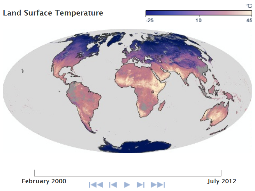
Unlike nominal- and ordinal-level data, which are categorical (qualitative) in nature, interval level data are numerical (quantitative). Examples of interval level data include temperature and year. With interval level data, the zero point is arbitrary on the measurement scale. For instance, zero degrees Fahrenheit and zero degrees Celsius are different temperatures.
4.2.4 Ratio Level
Similar to interval level data, ratio level data are also numerical (quantitative). Examples of ratio level data include distance and area (e.g., acreage). Unlike the interval level measurement scale, the zero is not arbitrary for ratio level data. For example, zero meters and zero feet mean exactly the same thing, unlike zero degrees Fahrenheit and zero degrees Celsius (both temperatures). Ratio level data also differs from interval level data in the mathematical operations that can be performed with the data. An implication of this difference is that a quantity of 20 measured at the ratio scale is twice the value of 10 (20 meters is twice the distance of 10 meters), a relation that does not hold true for quantities measured at the interval level (20 degrees is not twice as warm as 10 degrees).
4.2.5 Interval and Ratio Level Data
The scales for both interval and ratio level data are similar in so far as units of measurement are arbitrary (Celsius versus Fahrenheit and English versus metric units). These units of measurement are split evenly for each successive value (e.g., 1 meter, 2 meters (add 1 meter), 3 meters (add 1 meter), 4 meters (add 1 meter). Because interval and ratio level data represent positions along continuous number lines, rather than members of discrete categories, they are also amenable to analysis using statistical techniques.
Try This: Surf the Internet and find an interesting map, visualizing data from two of the different attribute measurement scales: nominal, ordinal, interval, and ratio. Provide a written citation for the source of each map as well as one sentence describing how each map uses nominal, ordinal, interval or ratio level data.
4.2.6 Attribute Measurement Level Operations
One reason that it's important to recognize levels of measurement is that different analytical operations are possible with data at different levels of measurement (Chrisman 2002). Some of the most common operations include:
- Group: Categories of nominal and ordinal data can be grouped into fewer categories. For instance, grouping can be used to reduce the number of land use/land cover classes from, for instance, four (residential, commercial, industrial, parks) to one (urban).
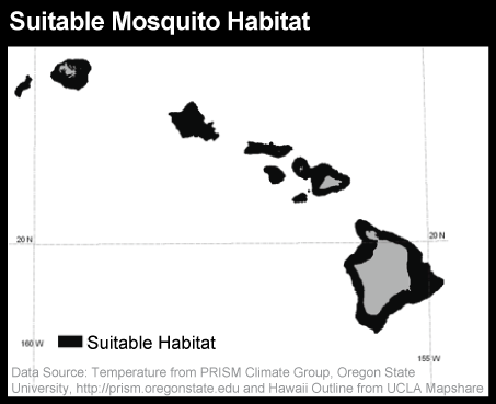
- Isolate: One or more categories of nominal, ordinal, interval, or ratio data can be selected, and others set aside. For example, consider a range of temperature readings taken over a large area. Only a subset of those temperatures are suitable for mosquito survival, and health officials can select and isolate areas based upon a specific temperature range that is likely there to take action in order to reduce the threat of a West Nile Virus or Dengue Fever outbreak from these mosquitoes.
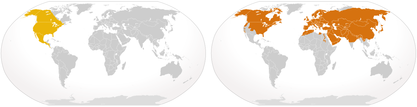
- Difference: The difference of two interval-level observations (such as two calendar years) can result in one ratio level observation (such as one age). For example, in 2012 (a year is an interval level value), someone born in 2000 (also interval level, of course) is 12 years old (age is ratio level since it has a definite zero).
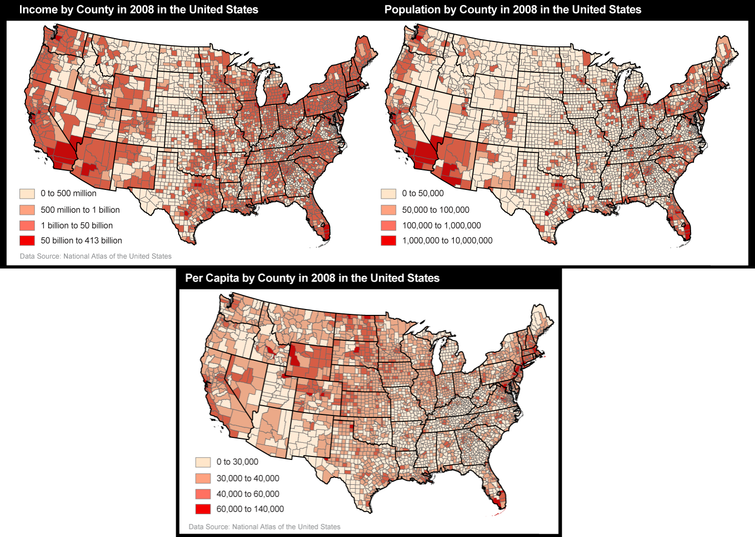
- Other arithmetic operations: Two or more compatible sets of interval or ratio level data can be added or subtracted. Only ratio level data can be multiplied or divided. For example, the per capita (average) income of an area can be calculated by dividing the sum of the income (ratio level) of every individual in that area (ratio level), by the number of persons (ratio level) residing in that area (a second ratio level variable).
- Classification: Numerical data (at interval and ratio level) can be sorted into classes, typically defined as non-overlapping numerical data ranges as discussed in Chapter 3.2.6. These classes are frequently treated as ordinal level categories for thematic mapping with the symbolization on choropleth maps, for example, emphasizing rank order without attempting to represent the actual magnitudes.
Practice Quiz
Registered Penn State students should return now take the self-assessment quiz Features and Attributes.
You may take practice quizzes as many times as you wish. They are not scored and do not affect your grade in any way.
4.3 Database Management Systems
Digital data are stored in computers as files. Often, data are arranged in tabular form. For this reason, data files are often called tables. A database is a collection of tables specifically designed for efficient retrieval and use. Businesses and government agencies that serve large clienteles, such as telecommunications companies, airlines, credit card firms, and banks, rely on extensive databases for their billing, payroll, inventory, and marketing operations. Database management systems (DBMS) are information systems that people use to store, update, and analyze non-geographic databases.
Often, data files are composed of rows and columns. Rows, also known as records, correspond to individual entities, such as a customer account or a city. Columns correspond to the various attributes associated with each individual entity. The attributes stored in the accounts database of a telecommunications company, for example, might include customer names, telephone numbers, addresses, current charges for local calls, long distance calls, taxes, etc.
Geographic data are a special case: records typically correspond with places. Columns represent the attributes of places. The data in the following table, for example, consist of records for Pennsylvania counties. Columns contain selected attributes of each county, including the county's ID code (FIPS code), name (County), and 1980 population (1980 Pop).
| FIPS Code | County | 1980 Pop |
|---|---|---|
| 42001 | Adams County | 78274 |
| 42003 | Allegheny County | 1336449 |
| 42005 | Armstrong County | 73478 |
| 42007 | Beaver County | 186093 |
| 42009 | Bedford County | 47919 |
| 42011 | Berks County | 336523 |
| 42013 | Blair County | 130542 |
| 42015 | Bradford County | 60967 |
| 42017 | Bucks County | 541174 |
| 42019 | Butler County | 152013 |
| 42021 | Cambria County | 163062 |
| 42023 | Cameron County | 5913 |
| 42025 | Carbon County | 56846 |
| 42027 | Centre County | 124812 |
Figure 4.9: The contents of one file in a database
Credit: Department of Geography, The Pennsylvania State University.
The example is a small and very simple file, but many geographic attribute databases are in fact large and complex (the U.S. is made up of over 3,000 counties, almost 50,000 census tracts, about 43,000 five-digit ZIP code areas and many tens of thousands more ZIP+4 code areas). Large databases consist not only of lots of data, but also lots of files. Unlike a spreadsheet, which performs calculations only on data that are present in a single document, database management systems allow users to store data in, and retrieve data from, many separate tables (which might be stored within a single database or perhaps as separate files). For example, suppose an analyst wished to calculate population change for Pennsylvania counties between the 1980 and 1990 censuses. More than likely, 1990 population data would exist in a separate table, like so:
| FIPS Code | 1990 Pop |
|---|---|
| 42001 | 84921 |
| 42003 | 1296037 |
| 42005 | 73872 |
| 42007 | 187009 |
| 42009 | 49322 |
| 42011 | 352353 |
| 42013 | 131450 |
| 42015 | 62352 |
| 42017 | 578715 |
| 42019 | 167732 |
| 42021 | 158500 |
| 42023 | 5745 |
| 42025 | 58783 |
| 42027 | 131489 |
Figure 4.10: Another file in a database. A database management system (DBMS) can relate this file to the prior one illustrated above because they share the list of attributes called "FIPS Code."
Credit: Department of Geography, The Pennsylvania State University.
A database management system (DBMS) can relate this table to the prior one illustrated above because they share the list of attributes called "FIPS Code." If two data table have at least one common attribute (e.g., FIPS Code), a DBMS can combine them in a single new table. The common attribute is called a key, and can be used for associating the individual records in the two tables. In this example, the key was the county FIPS code (FIPS stands for Federal Information Processing Standard), allowing the user to merge both tables into one. The DBMS also allows users to create new data such as the "% Change" attribute in the table below calculated from the 1980 and 1990 population totals that were merged together.
| FIPS | County | 1980 | 1990 | % Change |
|---|---|---|---|---|
| 42001 | Adams | 78274 | 84921 | 8.5 |
| 42003 | Allegheny | 1336449 | 1296037 | -3 |
| 42005 | Armstrong | 73478 | 73872 | 0.5 |
| 42007 | Beaver | 186093 | 187009 | 0.5 |
| 42009 | Bedford | 47919 | 49322 | 2.9 |
| 42011 | Berks | 336523 | 352353 | 4.7 |
| 42013 | Blair | 130542 | 131450 | 0.7 |
| 42015 | Bradford | 60967 | 62352 | 2.3 |
| 42017 | Bucks | 541174 | 578715 | 6.9 |
| 42019 | Butler | 152013 | 167732 | 10.3 |
| 42021 | Cambria | 163062 | 158500 | -2.8 |
| 42023 | Cameron | 5913 | 5745 | -2.8 |
| 42025 | Carbon | 56846 | 58783 | 3.4 |
| 42027 | Centre | 124812 | 131489 | 5.3 |
Figure 4.11: A new file produced from the prior two files as a result of two database operations. One operation merged the contents of the two files without redundancy. A second operation produced a new attribute--"% Change"--dividing the difference between "1990 Pop" and "1980 Pop" by "1980 Pop" and expressing the result as a percentage.
Credit: Department of Geography, The Pennsylvania State University.
Above, a new table is produced from the prior two tables as a result of two database operations. One operation merged the contents of the two tables. A second operation produced a new attribute--"% Change"--dividing the difference between "1990 Pop" and "1980 Pop" by "1980 Pop" and expressing the result as a percentage.
Database management systems provide a simple but powerful language that makes data retrieval and manipulation easy. These data can be retrieved and manipulated based upon user specified criteria, enabling users to select data in response to particular questions. A question that is addressed to a database through a DBMS is called a query. In addition, DBMS are valuable because they provide secure means of storing and updating data. Database administrators can also protect files so that only authorized users can make changes and provide transaction management functions that allow multiple users to edit the database simultaneously.
Database queries include basic set operations, including union, intersection, and difference. The product of a union of two or more data files is a single file that includes all records and attributes for features that appear in one file or the other, with records in common merged to avoid repetition. For example, if one wanted to find what both the coyote and red fox could prey upon, you can perform a union by combining the entire area that encompasses the territory of the coyote and the red fox.
An intersection produces a data file that contains only records that are present in all files. This is the area where both animals may compete for food, or where they overlap in territory. A difference operation produces a data file that eliminates records that appear in both original files. The difference of the red fox territory and the coyote territory produces places in which the predation may be lower and the stress of competition less.
Try This
Draw Venn diagrams--intersecting circles that show relationships between two or more entities--to illustrate the three operations. Then compare your sketch to this one [6].) As mentioned earlier in the chapter, all operations that involve multiple data files rely on the fact that all files contain a common key. The key allows the database system to relate the separate files. Databases that contain numerous files that share one or more keys are called relational databases. Database systems that enable users to produce information from relational databases are called relational database management systems. In the example above, if data on foxes and coyotes were aggregated to watersheds, then the watershed specification could act as the geographic key for connecting the two sets of data.
4.3.1 Available Tools
Numerous tools exist to help users perform database management operations. Microsoft Excel and Access allow users to retrieve specific records, manipulate the records, and create new user content. ESRI’s ArcGIS allows users to query and manipulate files, but also map the geographic database files in order to find interesting spatial patterns and processes in graphic form.
4.4 Metadata
Metadata, simply stated, is data about data. It is used to document the content, quality, format, ownership, and lineage of individual data sets. Perhaps the most familiar example of metadata is the "Nutrition Facts" panel printed on food and drink labels in the U.S.
Try This:
Visit the Pennsylvania Spatial Data Access site [7]. This is the website for the Pennsylvania Spatial Data Access (PASDA) geospatial data clearinghouse (built by Penn State). PASDA provides access to a wide array of spatial data for Pennsylvania as a whole and places within the state. Click on “Statewide Data [8]” in the link under "Quick Links" at the bottom left of the page. You will see a list of many state-wide data sets. All can be downloaded (by clicking the disk icon) and are usable by multiple map services (lightning icon). Some have data viewers available (globe icon) and some can be added to a “cart” for mapping (plus icon). Click on a copy of the titles. You will see some basic metadata; what categories are included for all entries? Then, click on “View Full Metadata” to see an example of the kinds of detailed metadata that has been recorded. Users of the site can also download this metadata description as an XML file for later use.
Some metadata also provide the keywords needed to help users search for available data in larger specialized clearinghouses and in the World Wide Web. Going back to the PASDA site, look in the upper right; you will see a “Data Search” facility. Try a term such as “water”, “school”, or others that you might expect to see data for. If the term has been used in the database metadata, the data set will be listed.
In 1990, the U.S. Office of Management and Budget issued Circular A-16, which established the Federal Geographic Data Committee (FGDC) as the interagency coordinating body responsible for facilitating cooperation among federal agencies whose missions include producing and using geospatial data. FGDC is chaired by the Department of Interior, and is administered by United States Geological Survey (USGS).
In 1994, President Bill Clinton’s Executive Order 12906 charged the FGDC with coordinating the efforts of government agencies and private sector firms leading to a National Spatial Data Infrastructure (NSDI). The Order defined NSDI as "the technology, policies, standards and human resources necessary to acquire, process, store, distribute, and improve utilization of geospatial data" (White House, 1994). It called upon FGDC to establish a National Geospatial Data Clearinghouse, ordered federal agencies to make their geospatial data products available to the public through the Clearinghouse, and required them to document data in a standard format that facilitates Internet search. Agencies were required to produce and distribute data in compliance with standards established by FGDC. (The Departments of Defense and Energy were exempt from the order, as was the Central Intelligence Agency.)
Some of the key components included in the FGDC metadata standard include:
- identification information: who created the data, a brief description of its content, form, and purpose; its status, spatial extent, and use restrictions;
- data quality information: accuracy and completeness of attributes, horizontal and vertical positions, sources, and procedures used to create the data;
- spatial reference information: projection and/or coordinate system; datum and ellipsoid;
- entity and attribute information: feature and attribute categories used; and
- distribution information: availability, and how to acquire the data.
FGDC's Content Standard for Digital Geospatial Metadata is published at the FGDC standards publication site [9]. Geospatial professionals understand the value of metadata, know how to find it, and how to interpret it.
Practice Quiz
Registered Penn State students should return now take the Chapter 4 practice quiz in Canvas: Metadata and Databases.
You may take practice quizzes as many times as you wish. They are not scored and do not affect your grade in any way.
4.5 Vector Versus Raster
Innovators in many fields, including engineers, computer scientists, geographers, and others, started developing digital mapping systems in the 1950s and 60s. One of the first challenges they faced was to convert the graphical data stored on paper maps into digital data that could be stored in, and processed by, digital computers. Several different approaches to representing locations and extents in digital form were developed. The two predominant data representation strategies are known as "vector" and "raster."
Recall that data consist of symbols that represent measurements. Digital geographic data are encoded as alphanumeric symbols that represent locations and attributes of locations measured at or near Earth's surface. No geographic data set represents every possible location, of course. The Earth is too big, and the number of unique locations is mathematically infinite. In much the same way that public opinion is measured through polls, geographic data are constructed by measuring representative samples of locations. And just as serious opinion polls are based on sound principles of statistical sampling, so, too, do geographic data represent reality by measuring carefully chosen samples of locations. Vector and raster data are, in essence, two distinct sampling strategies: vector and raster.
The vector approach involves sampling either specific point locations, point intervals along the length of linear entities (like roads), or points surrounding the perimeter of areal entities (like water bodies such as lakes or oceans). When the points are connected by lines or arcs, the sampled points form line features and polygon features that approximate the shapes of their real-world counterparts.
 [10]
[10]
Try This:
Click the graphic above to download and view the animation file (vector.avi, 1.6 Mb) in a separate Microsoft Media Player window. View the same animation in QuickTime format (vector.mov, 1.6 Mb) here [11]. Requires the QuickTime plugin, which is available free at the Apple Quicktime download site [12].
The aerial photograph above left shows two entities, a reservoir and a highway. The graphic above right illustrates how the entities might be represented with vector data. The small squares are nodes: point locations specified by latitude and longitude coordinates. Line segments connect nodes to form line features. In this case, the line feature colored red represents the highway. A series of line segments that begin and end at the same node form polygon features. In this case, two polygons (filled with blue) represent the reservoir.
The vector data model is consistent with how surveyors measure locations at intervals as they traverse a property boundary. The vector strategy is well suited to mapping entities with well-defined edges, such as highways or pipelines or property parcels. Many of the features shown on paper maps, including transportation routes, rivers, and political boundaries, can be represented effectively in digital form using the vector data model.
The raster approach involves sampling attributes for a set of cells having a fixed size. Each sample represents one cell, or pixel, in a checkerboard-shaped grid, as shown in Figure 4.14 below. The cells shown are square, but raster data can be generated with any regular subdivision into interconnected, non-overlapping cells that are identical in shape. While most raster data use square cells, rectangular and hexagonal cells are also encountered.
Try This:
Click the graphic above to download and view the animation file (raster.avi, 0.8 Mb) in a separate Microsoft Media Player window. View the same animation in QuickTime format (raster.mov, 0.6 Mb) here [13]. Requires the QuickTime plugin, which is available free at at the Apple Quicktime download site [12].
The graphic above illustrates a raster representation of the same reservoir and highway as shown in the vector representation. The area covered by the aerial photograph has been divided into a grid. Every grid cell that overlaps one of the two selected entities is encoded with an attribute that associates it with the entity it represents. Actual raster data would not consist of a picture of red and blue grid cells, of course; they would consist of a list of values (either categorical or numerical), one value for each grid cell, each number representing an entity. For example, grid cells that represent the highway might be represented with the value "1" or “H” (either of which could be used to represent the highway category) and grid cells representing the reservoir might be coded with the value "2" or “R” (representing the reservoir category).
The raster strategy is a smart choice for representing phenomena that lack clear-cut boundaries, such as terrain elevation, vegetation, and precipitation. Digital airborne imaging systems, which are replacing photographic cameras as primary sources of detailed geographic data, produce raster data by scanning the Earth's surface pixel by pixel and row by row. This will be discussed in more detail in Chapter 8, Info Without Being There: Imaging Our World.
Both the vector and raster approaches accomplish the same thing: they allow us to represent the Earth's surface with a limited number of locations. What distinguishes the two is the sampling strategies they embody. The vector approach is like creating a picture of a landscape with shards of stained glass cut to various shapes and sizes. The raster approach, by contrast, is more like creating a mosaic with tiles of uniform size. Neither is well suited to all applications, however. Several variations on the vector and raster themes are in use for specialized applications, and the development of new object-oriented approaches is underway.
Practice Quiz
Registered Penn State students should return now take the Chapter 4 practice quiz in Canvas to take a self-assessment: Vector Versus Raster.
You may take practice quizzes as many times as you wish. They are not scored and do not affect your grade in any way.
4.6 Summary
This chapter introduced the characteristics of digital data and how they are represented. These representations included data storage, management, and manipulation, leading to new insights and information. We have identified the difference between a feature (or object) and its associated attributes that describe the feature. The four attribute measurement scales (nominal, ordinal, interval, and ratio) enable social scientists to systematically measure and analyze phenomena that cannot simply be counted. These levels, which subdivide the categorical and numerical distinctions introduced in previous chapters, are important to specialists in geographic information because they provide guidance about the proper use of different operations and mapping techniques. Many of these operations are carried out in a database management system, allowing users to query, store, merge, and manipulate data to create new information within numerous available systems that offer varying levels of sophistication in analysis. A key type of data discussed in this chapter is metadata, or the data about the data. Metadata includes documentation of the content, quality, format, ownership, and lineage of individual data sets. Finally, the chapter ended with introduction of two predominant data representation strategies, known as vector and raster. Both approaches allow us to represent the real world in digital form through representative samples of locations. Most maps that you encounter online or on your smart phones and related devices are generated from data collected and organized using one or both representation forms.
4.7 Glossary
Attribute: Data about a geographic feature often found in geographic databases and typically represented in the columns of the database.
Classification: Numerical data (at interval and ratio level) sorted into classes, typically defined as non-overlapping numerical data ranges.
Database: A collection of tables specifically designed for efficient retrieval and use.
Database Management System: Information systems that people use to store, update, and analyze non-geographic databases.
Difference: A data operation that produces a set of entities that appear in only one of two sets; thus it eliminates records that appear in both original sets.
Geographic Information Systems (GIS): A computer-based tool used to help people transform geographic data into geographic information.
Group: An attribute measurement level operation that combines data into fewer categories.
Information Systems: Computer-based tools that help people transform data into information.
Intersection: A data file that contains only records that are present in all files.
Interval Level Data: Numerical data with an arbitrary zero point on the measurement scale.
Isolate: The operation of selecting specific data and isolating it while setting other parts of the data aside.
Key: A common attribute among multiple databases/files that allow the database system to relate the separate files.
Level of Measurement: A systematic approach to data measurement for phenomena, as it cannot simply be counted.
Metadata: Data about data to document the content, quality, format, ownership, and lineage of individual data sets.
Nodes: Point locations specified by latitude and longitude coordinates.
Nominal Level Data: Data that are denoted with different names or categories.
Ordinal Level Data: The assignment of ranked or ordered observations to discrete categories.
Qualitative: A type of data that is based on a quality or characteristic.
Quantitative: A type of data that is based on quantities.
Query: A question or code addressed to the database for certain information.
Raster: Involves sampling attributes for a set of cells having a fixed size.
Ratio Level Data:Numerical data where the zero is not arbitrary on the measurement scale.
Records: Often rows in a database table, corresponding to individual entities.
Relational Database: Databases that contain numerous files that share one or more keys.
Relational Database Management Systems: Database systems that enable users to produce information from relational databases.
Spatial Queries: Questions addressed to a database, such as wanting to know a distance or the location where two objects intersect.
Standard Query Language: A programming language used in database management systems.
Table: Data arranged in tabular form.
Union: A single file that includes all records and attributes for features that appear in one file or the other, with records in common merged to avoid repetition.
Vector: Involves sampling either specific point locations, point intervals along the length of linear entities, or points surrounding the perimeter of areal entities, resulting in point, line, and polygon features.
4.8 Bibliography
Brewer, C. & Suchan, T., (2001). Mapping census 2000: The geography of U. S. diversity. U. S. Census Bureau, Census Special Reports, Series CENSR/01-1. Washington, D. C.: U.S. Government Printing Office.
Chrisman, N. (1997). Exploring geographic information systems. New York: John Wiley & Sons, Inc.
Chrisman, N. (2002). Exploring geographic information systems. (2nd ed.). New York: John Wiley & Sons, Inc.
Goodchild, M. (1992). Geographical information science. International Journal of Geographic Information Systems 6:1, 31-45.
National Decision Systems. A zip code can make your company lots of money! Retrieved on July 6, 1999, from http://laguna.natdecsys.com/lifequiz [14] (since retired).
Steger, T. D. (1986). Topographic maps. Washington D.C.: U.S. Government Printing Office.
Stevens, S.S. (1946). On the theory of scales of measurement. Science, 103, 677-680.1
U.S. Geological Survey (2012) Topographic Map Symbols, ISBN 0-607-96942-3; available at: https://pubs.usgs.gov/gip/TopographicMapSymbols/topomapsymbols.pdf [15]
Worboys, M. F. (1995). GIS: A computing perspective. London: Taylor and Francis.