Section 3: Systems Approaches to Managing our Food Systems
Section 3: Systems Approaches to Managing our Food Systems
Overview
This is the third section of the course, where you will deepen your understanding of the connections between the natural environment and the human food production system. We already learned how important soil resources, water resources, and climate are in determining which crops we can grow and where we can grow them. In this section, we explore more soil management strategies and start to learn more about pests and climate change, which are two significant stressors for our human food system. Module 7 delves deeper into the management of soils and crops to improve soil quality for agriculture and illustrates more connections between natural systems and human systems. In Module 8, you'll explore types of pests and different methods used to manage pests as well as some of the challenges and opportunities to sustainably manage pests. The last module in this section, Module 9, first introduces the science of global climate change, then examines future projects for key climate variables that influence food production. Finally, the section wraps up with Stage 3 of the capstone, in which you'll explore each of these topics in relation to your capstone region.
Modules
- Module 7: Soils and a Systems Approach to Soil Quality
- Module 8: Pests and Integrated Pest Management
- Module 9: Climate change
- Capstone Stage 3
Section Goals
Upon completion of Section 3 students will be able to:
- Understand the human impact on the environment in food systems and natural system feedbacks.
- Apply broadly the principles of sustainable soil management in proposing solutions for food systems.
- Apply an understanding of vulnerability, food insecurity, and diet quality as human system properties that determine food system sustainability.
- Analyze a wide variety of food system types from the standpoint of human-natural interaction.
- Critique food systems based on an understanding of food system properties related to resilience, adaptive capacity, and vulnerability.
- Incorporate contributions of Food System-oriented movements and their proposals into their food system proposals.
- Propose an integrated plan or scenario for the sustainability of an example food system (capstone project).
- Learn the types and features of major agricultural insect pests, the benefits of insects, challenges associated with pest control.
- Learn how trophic interactions can contribute to pest control, and the scientific basis for IPM to control agricultural pests over the long term.
- Understand weed and pathogen pests.
- Learn how integrated pest and weed management can contribute to long-term successful weed and pest management, and some transgenic pest management technologies and their impact.
Section Objectives
In order to reach these goals, we have established the following learning objectives for student learning. Upon completion of the modules within Section 3, you will be able to:
- Name different food system impacts on earth's natural systems.
- Define and provide an example of sustainable soil management practices including tillage, soil erosion prevention, cover cropping and crop rotational diversity.
- Describe different options for sustainable water use in food systems.
- Describe food systems as coupled natural-human systems.
- Describe the three major types of food systems in the world today.
- Describe a life cycle analysis and what it is used for.
- Describe characteristics of insect pests and factors that make them successful pests, as well as beneficial characteristics of insects.
- Explain some history of agricultural pesticides.
- Describe factors that contribute to pests evolving resistance to pest control strategies.
- Discuss what IPM is and why it is effective.
- Interpret how to apply the pest scouting data and distinguish if pests have reached an economic threshold.
- Analyze IPM management scenarios and interpret the agroecosystem benefits of IPM.
- Describe and compare the characteristics of natural ecosystems and agroecosystems, and explain how trophic level interactions and biodiversity may contribute to pest control.
- Describe characteristics of weed pests and factors that make them successful pests, as well as beneficial characteristics of weeds.
- Describe categories of weed management tactics with example weed control practices.
- Explain what organisms and factors contribute to crop diseases.
- Explain some recent transgenic pest management technologies and analyze and interpret scientific data about transgenic technologies.
- Differentiate pest control approaches that are likely to be effective in the long term based on IPM principles, and generate or formulate IPM approaches to enhance pest control.
- Describe the evolutionary changes in the human history of diets and the current changes in modern globalized diet contexts.
- Define concepts related to food security and resilience in food systems such as adaptive capacity, food access, vulnerability, and malnutrition.
- Distinguish different ways that food systems develop and change because of interacting natural and human factors.
- Discuss how managing crops and soils as a system promotes soil quality and multiple agroecosystem benefits and makes food systems.more productive and sustainable.
- Apply and interpret a life cycle assessment (LCA) to measure and compare system impacts on earth's natural systems.
- Analyze mapping resources related to food access and food insecurity.
- Analyze the causes and historical trajectory of an example of a famine.
- Evaluate and compare different approaches to deal with water scarcity in food systems.
- Propose strategies for improved water use, soil management, system resilience, and diet improvement as part of an integrated strategy for food system sustainability.
Module 7: Soils and a Systems Approach to Soil Quality
Module 7: Soils and a Systems Approach to Soil Quality
Introduction
There are multiple soil conservation practices that can reduce soil erosion and improve soil quality. In this module, you will explore what is meant by soil quality or soil health for agricultural production, as well as how strategic crop selection, crop sequencing, and reduced soil tillage practices in combination are most effective for improving soil quality for agriculture.
Goals and Learning Objectives
Goals and Learning Objectives
Goals
- Describe different types of cropping systems types, soil tillage practices, and indicators of soil quality.
- Interpret the effect of cropping systems and soil tillage approaches on soil conservation and quality.
- Distinguish which crop and soil management practices promote soil health and enhanced agroecosystem performance.
Learning Objectives
After completing this module, students will be able to:
- Define and provide an example of some cropping system practices (ex. monoculture, double crop, rotation, cover crop, intercrops).
- Define soil quality and describe some indicators of soil quality.
- Explain some tillage systems and how tillage practices affect soil quality.
- Interpret how the integration of cropping and tillage systems can promote soil conservation and quality.
- Analyze and prescribe some cropping systems and tillage practices that promote soil quality and other agroecosystem benefits.
Assignments
Module 7 Roadmap
Detailed instructions for completing the Summative Assessment will be provided in each module.
| Action | Assignment | Location |
|---|---|---|
| To Read |
|
|
| To Do |
|
|
Questions?
If you prefer to use email:
If you have any questions, please send them through Canvas e-mail. We will check daily to respond. If your question is one that is relevant to the entire class, we may respond to the entire class rather than individually.
If you prefer to use the discussion forums:
If you have any questions, please post them to the discussion forum in Canvas. We will check that discussion forum daily to respond. While you are there, feel free to post your own responses if you, too, are able to help out a classmate.
Module 7.1: Cropping Systems and Soil Quality
Module 7.1: Cropping Systems and Soil Quality
Introduction
Plants and soil interact; soil provides water and nutrients to plants, and plant roots contribute organic matter to the soil, can promote soil structure, and support soil organisms. Above ground crop residues (non-harvested plant parts such as stems and leaves) can also protect the soil from erosion and return organic matter to the soil. But soil tillage can make soil vulnerable to erosion, alter soil physical properties and soil biological activity. In Module 7.1, you will learn what is meant by soil health for agricultural production and explore how crop types and cropping systems can impact the soil.
Cropping Systems
Cropping Systems
Recall in module 5, we examined how soils, climate, and markets play major roles in determining which crops farmers cultivate. In many cases, farmers cultivate multiple crops of more than one life-cycle because the diversity provides multiple benefits, such as soil conservation, interruption of pest lifecycles, diverse nutritional household requirements, and reduced market risk. In this module, we examine some ways that farmers cultivate crops in sequence and define some of the terms for this crop sequencing.
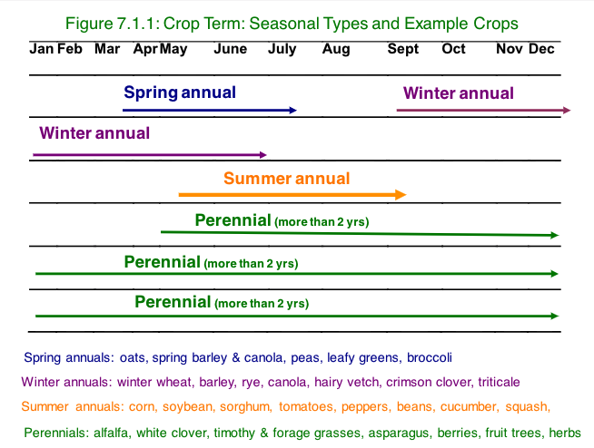
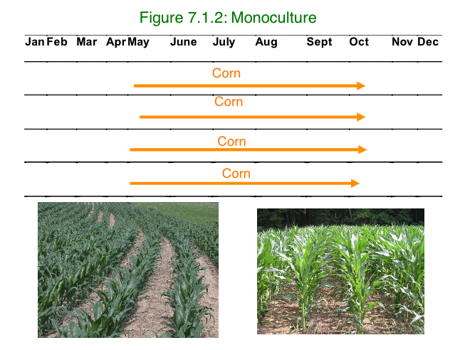
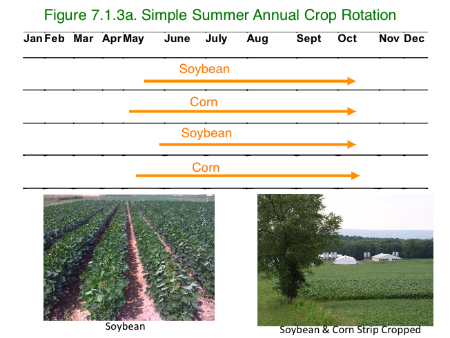
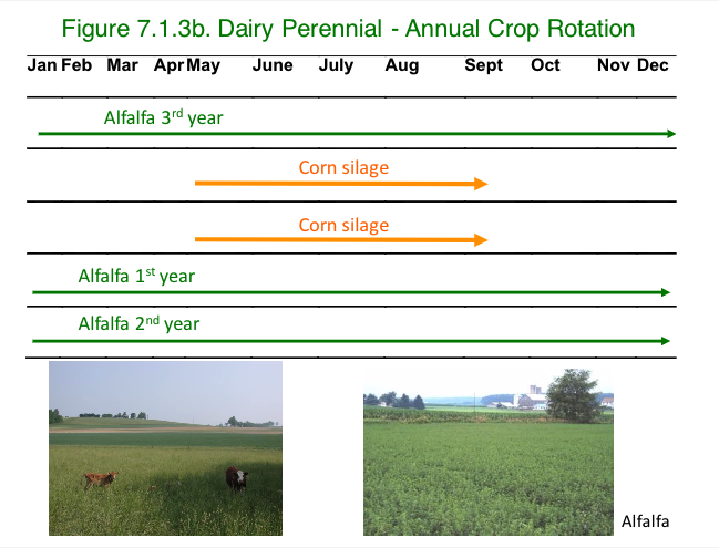
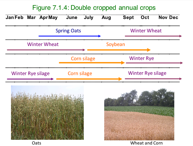
A sole crop refers to planting one crop in a field at a time. Recall from Module 5, the seasonal crop types (Figure 7.1.1) and note that different seasonal crops could be planted in succession. A monoculture refers to planting the same crop year after year in sequence (See Figure 7.1.2). By contrast in a crop rotation, different crops are planted in sequence within a year or over a number of years, such as shown in Figures 7.1.3a and 7.1.3b. When two crops are planted and harvested in one season or slightly more than one season, the system is referred to as double cropping, as illustrated in Figure 7.1.4. Where growing seasons are long and/or crop life cycles are short (ex. leafy greens), three crops may be planted in sequence within a season, as a triple-crop.
Crop rotations and double cropping can provide many soil conservation and soil health benefits that are discussed in the reading assignment at the end of this page, and in Module 7.2. Crop rotations can provide additional pest control benefits particularly when crops from different plant families are rotated, as different families typically are not hosts of the same insect pest species and crop pathogens. Integrating crops of different seasonal types and life cycles in a crop rotation also interrupts weed life cycles by alternating the time when crops are germinating and vulnerable to weed competition. Rotating annual crops with perennial forage crops that are harvested a couple of times in a growing season also interrupts annual weed life cycles, because most annual weeds don't survive the frequent forage crop harvests.
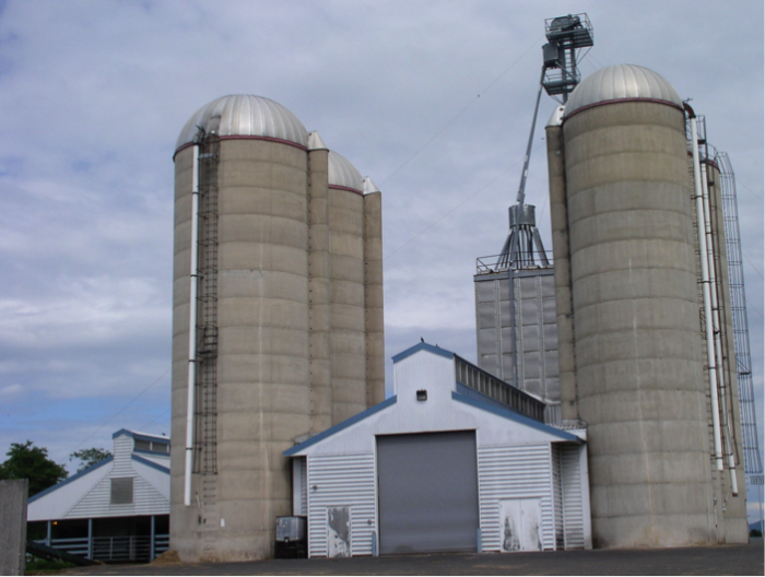
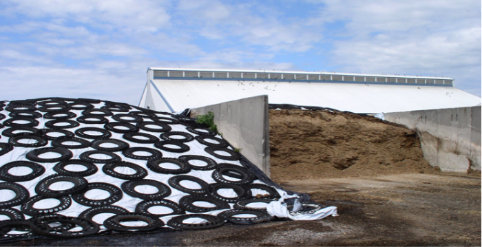
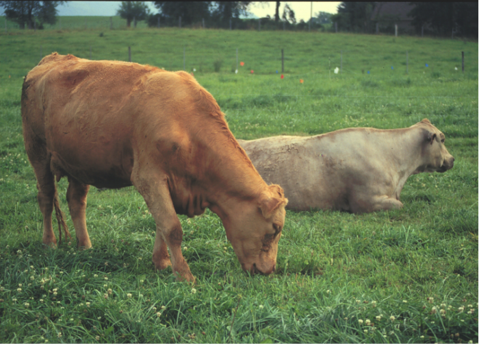
When all or most of a crop is grazed or harvested for feed for ruminant livestock, such as dairy and beef cattle or sheep, the crop is referred to as a forage crop. Examples of forage crops include hay and pasture crops, as well as silage that can be produced from perennial crops and most grain crops. For instance, silage from alfalfa, perennial grass species, corn, oat, and rye is made when most of the aboveground plant material (leaves, stems and grain in the case of grain crops) is harvested and fermented in a storage structure called a silo or airtight structure. To preserve the silage, air is precluded from the storage structure and microbes on the plant material initially feed on the crop tissues, deplete oxygen in the storage structure, and produce acidic byproducts that decrease the pH of the forage. This acidic environment without oxygen prevents additional micro-organisms from growing, effectively "pickling", and preserving the forage.
Intercrops and Cover Crops
Intercrops and Cover Crops
Intercrops are two or more crops that are planted together in a field at the same time or to be planted close in time and overlap for some or all of their life cycle. Intercrops may provide a range of benefits including: i. improving soil fertility, ii. increasing crop diversity and iii. reducing pest pressure. The mixtures also often produce higher yield and crop quality. There are multiple types of intercrops that vary in their spatial arrangement.
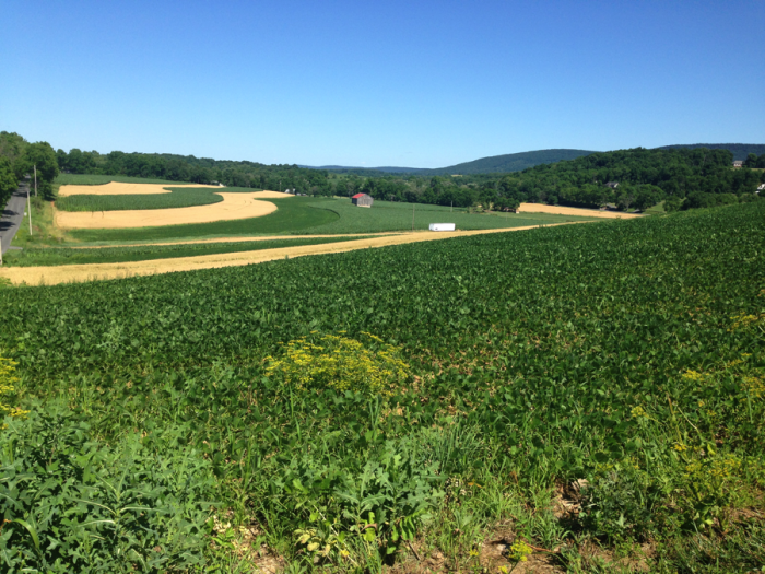
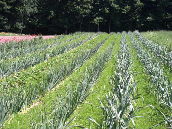
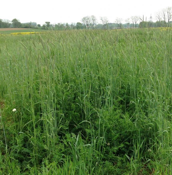
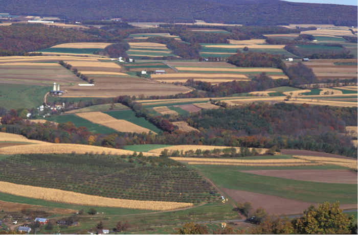
Strip intercrops are wide strips with multiple rows of one crop, that are alternated on the field with strips of one or more different crop(s). Strip intercrops are typically planted on the field contour with crops of different life cycles that protect soil from erosion throughout the year. For instance, strips of corn may be alternated with strips of perennial forage grasses that can reduce soil erosion across the field when the corn isn't growing. Or, as in the photo below, winter wheat provided live plant coverage on portions of the field in spring, prior to corn and soybean were planted. In mid-summer, corn and soybean provide live coverage after wheat is harvested; and in fall, winter wheat will be growing on some strips after corn and soybean are harvested. Having strips of different crop species can also reduce the spread of insect pests and crop pathogens compared to cultivating one crop on the entire field.
Row intercrops alternate rows of different crop species, usually every other row or every two rows.
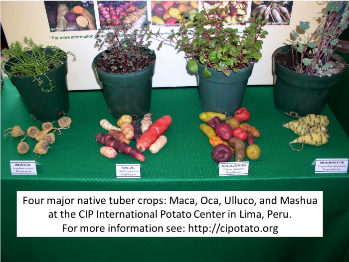
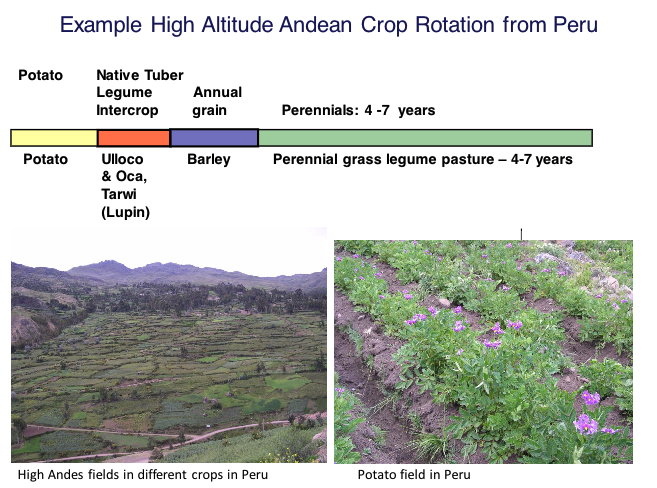
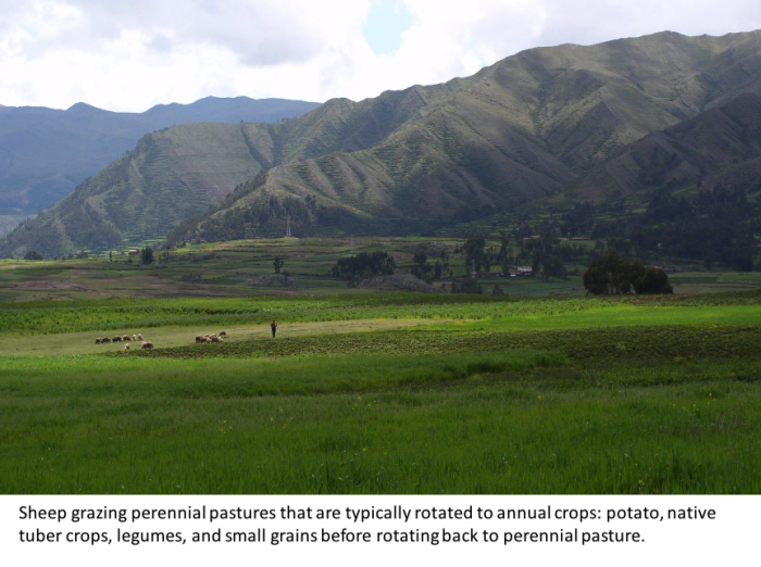
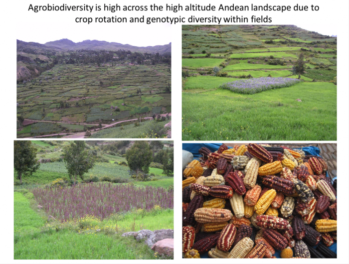
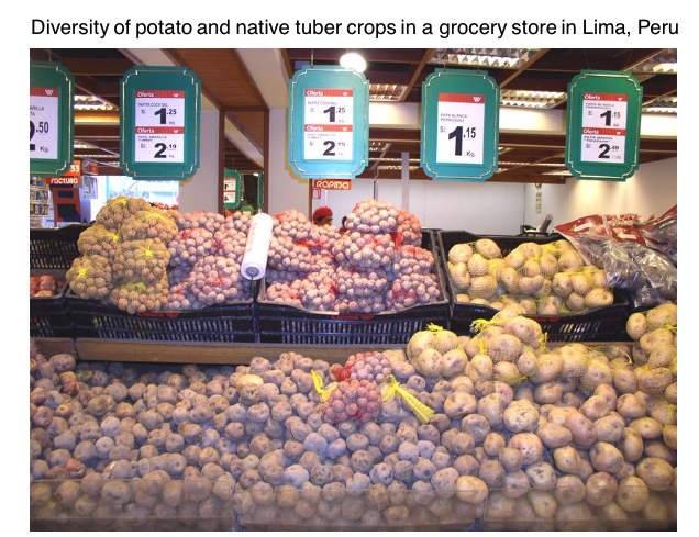
Mixture intercrops tend to be combined randomly when planted; such as grass and legume forage mixtures. Intercrops of different crop species (ex. native tuber mixtures) or different varieties of a crop species (ex. rice) are sometimes planted to reduce pathogen and insect pest infestations. Crop rotation and intercropping increase agrobiodiversity across an agricultural landscape, providing multiple potential agroecosystem benefits, such as i. reducing the risk of crop loss to pests and climatic stresses (ex. frosts, floods, and drought), ii. providing habitat for beneficial organisms such as pollinators and pest predators, and iii. enhancing the diversity of nutritional crops for farmers and markets. Further, integrating crops from the grass family tends to promote soil structure, while legumes enhance soil nitrogen, and integrating perennial crops protects the soil from erosion and builds soil organic matter and soil biological activity because perennials allocate a high proportion of their growth to storage organs. For instance, the photos below illustrate how both intercropping and crop rotation enhance agrobiodiversity in the high Andes of Peru.
Cover Crop: A cover crop is planted after a crop that is harvested and is terminated before the subsequent crop is planted. Cover crops tend to be annual crops that they can quickly establish after a harvested crop to protect the soil from erosion and provide other benefits including i. to add organic matter to the soil; ii. to scavenge nutrients and prevent nutrients from leaching out of the topsoil (also called a catch crop); iii. to support soil organisms in the root zone, iv. to suppress weeds, and v. to provide habitat for aboveground beneficial organisms, such as insects that predate on crop pests or weed seeds. Leguminous cover crops also add nitrogen to the soil when they are terminated and returned to the soil and are therefore often referred to as green manure crops. Cover crops are also sometimes referred to as "catch crops" because they can take up and retain nitrogen and other nutrients that might otherwise leach out of the rooting zone and be lost to deeper soil profiles, and potentially to groundwater.
Cover Crop Intercrops
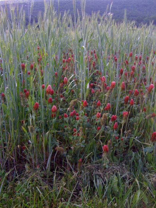
Because cover crop species have different plant traits that provide different cropping system benefits, often two or more species of cover crops are planted together as a cover crop intercrop or cover crop mixture. For instance, small grains that scavenge nitrogen well and have fibrous roots that bind soil particles and promote soil structure are often mixed with tap-rooted legumes that fix nitrogen. Some cover crop mixtures combine plant species that establish quickly in the late summer or early fall but don't typically survive the winter, such as oats or deep-rooted radish species. Non-winter hardy species are sometimes combined with winter-hardy species such as hairy vetch, cereal rye or annual ryegrass that survive the winter and provide cover in early spring.
Readings
Download the book Building Soils for Better Crops. Edition 3 [4]. Sustainable Agriculture Network, USDA. Beltsville, MD or read it online, Building Soils for Better Crops. Edition 3 [1].
For this module, you will be assigned to read multiple sections. So, we recommended that you download the book. Then, read more about the benefits of cover crops in Chapter 10: Cover Crops and Chapter 11: Crop Rotations.
Soil Quality, Soil Health
Soil Quality, Soil Health
As discussed in Module 5, soil is a complex matrix of minerals, air, water, organic matter, and living organisms. Historically, the emphasis in agriculture has been on reducing soil erosion. But since the 1990s, soil scientists and conservationists have recognized and described multiple valuable properties and ecosystem functions of soil that are referred to as indicators of soil quality or soil health. In 1997, the Soil Science Society of America's Ad Hoc Committee on Soil Quality (S-581) defined Soil Quality as:
"the capacity of a specific kind of soil to function, within natural or managed ecosystem boundaries, to sustain plant and animal productivity, maintain or enhance water and air quality, and support human health and habitation" (Karlen et al., 1997).
Indicators or measures of soil quality describe a soil's biological, chemical and physical properties. In addition to the soil chemical properties such as nutrient content and pH, additional indicators of soil quality include a soil’s:
- Organic matter content. Organic matter stores carbon can release nutrients, support soil biological activity, buffer soil pH, hold plant nutrients, and increase a soil's water-holding capacity
- Biological activity in the soil. Soil organisms can provide multiple benefits such as nutrient cycling, secreting sticky polysaccharides that help bind together soil particles and increase soil porosity and predation, and suppression of plant pests such as plant pathogens and weed seeds.
- Soil structure and porosity. Soils with good structure and porosity can support water and air infiltration and resist compaction. Water stable aggregates are an important physical indicator of soil health. Water stable aggregates contain soil mineral particles such as sand, silt, and clay that are typically held together by a combination of binding materials including fine root hairs, soil fungal hyphae (fungal filaments), and sticky polysaccharides that are exuded from soil microorganisms. Because they are stable when wet (during or after a precipitation event) they maintain soil pores that can contain and allow air and water to infiltrate the soil, reducing water and soil run-off. Water stable aggregates can also protect organic matter from degradation and soil microorganisms from predatory micro-organisms.

Read
Chapter 1 (Healthy Soil) and Chapter 2 (Organic Matter: What it is and Why it’s so important?) from the book that you downloaded: Building Soils for Better Crops. Edition 3 [1]. Sustainable Agriculture Network, USDA. Beltsville, MD.
Then watch the following video about soil biology and list four kinds of soil organisms and how they influence soil.: The Living Kingdoms Beneath our Feet. (USDA NRCS) [5].
Video: International Year of Soils July: The Living Kingdoms Beneath Our Feet (2:08)
Module 7.2: Conservation Agriculture: A Systems Approach
Module 7.2: Conservation Agriculture: A Systems Approach
Tillage can incorporate soil amendments such as fertilizers; bury weed seeds and crop residues that may harbor diseases and insects; remove residue that insulates the soil and promotes soil warming and crop seed germination and growth. Tillage can also cause soil erosion, disrupt soil organisms and soil structure; and remove residues that slow water run-off and evaporation, conserving soil moisture. Conservation tillage practices can reduce or eliminate the need for tillage, and the integration of perennials and cover crops can also protect soil from erosion and contribute to improving soil quality. In Module 7.2, we explore tillage and cropping practices that farmers can employ and integrate to conserve and improve their soil for long-term farm productivity.
Tillage Impacts on Soil Health
Tillage Impacts on Soil Health
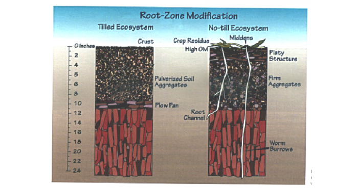
In addition to exposing soil to wind and water erosion, tillage can alter the physical structure, distribution of organic matter, and biological activity of soil. At the depth where the plow impacts the soil, a layer of soil compaction can develop (a plow pan), limiting water infiltration and plant rooting depth. Under tillage, crop residues, roots and root hairs, and their associated fungal hyphae are disturbed and more decomposed in the plow layer. By contrast, when roots, fine roots, and fungal hyphae are not disturbed and decomposed as rapidly, there are more channels that water, air, earthworms, and roots can move through, and soil aggregation is enhanced. Below is a schematic comparing the root zone profile of a conventionally tilled soil to a no-till soil.
Watch the three videos below, from USDA NRCS about soil tillage and soil health.
-
Video: The Science of Soil Health: What Happens When You Till? USDA NRCS (3:05)
Click for a transcript of the What Happens When You Till video.Interviewer: When we use tillage, the soil ecosystem is disturbed on a massive scale. Purdue's Dr. Eileen Kladivko contrasted natural ecosystems with tilled systems, and what we stand to lose when soils are tilled. Eileen: If you think about natural ecosystems, they don't have a tillage implement running through them once a year or a couple of times a year, but nutrients get recycled and trees grow or grasses grow and what's recycling the nutrients are the organisms. And so, part of what we're saying with a with a no-till system, is that if you don't take an implement through there, and you allow the system to kind of come back, that there will be organisms that will do that job for you. They do it differently, obviously than a piece of metal would do it, but they can be very effective. And besides loosening the soil or making burrows, they do some of these other things, like convert nutrients, ok, recycle nutrients, have pathways where roots can grow and then those pathways stay there. You know, if you think about a tillage implement, any root channel from last year in the topsoil, is going to be totally broken up by a tillage implement the next year. If you have a nightcrawler channel, or even if you have a red worm channel, that's part of the red worm channel, it's there and then the roots can follow that and so you can have channel built upon channel, built upon channel. And the nightcrawler channel, you know, maybe a root, maybe a corn root, maybe a cover crop root, will go down that, and the next year another nightcrawler, and so on. So it builds upon itself. Interviewer: Will you explain to us why organic matter decomposes faster because of tillage? Eileen: A tillage operation does a couple things, number one is it opens up aggregates that were otherwise protected. So you're opening up more surfaces for the bacteria to decompose the organic material faster. That's probably the main reason. Sometimes people say well you're putting oxygen in the soil. It's not really so much that, as by breaking up aggregates, you expose the organic matter in the soil to decomposition. Whereas when it's in an aggregated state in the soil, some of that's protected and the bacteria that decompose that organic matter can't get to it. Interviewer: So the tillage actually favors then, say bacteria, that would live in that environment. And that may be what causes the flush of carbon dioxide and nitrates into the soil as well. Eileen: Oh yes, yes, the flush of carbon dioxide is very much related to the tillage, right. -
Video: The Science of Soil Health: Nightcrawlers and Soil Water Flow. USDA NRCS (3:05)
Click for a transcript of the Nightcrawlers and Soil Water Flow video.Interviewer: When we get to those dry summer months, good soil hydrologic function is critical. We visited with Purdue University's Dr. Eilieen Kladviko to talk about the remarkable effect that nightcrawlers have on aiding water flow into and through soils. Interviewer: Well you’re a soil physicist Eileen, so we better talk about. Eileen: We better talk about water flow. Interviewer: Let’s talk about that water flow, because obviously water is a free resource to the farmer. Eileen: Right, in general our soils are excessively wet in the spring and that's more of our issue and that's why we use tile drainage (yes) and things like that. But what I'm getting at really is that the nightcrawlers, in particular, can be very important for getting infiltration of water into the soil during the growing season. So when we get those quick thunderstorms in the middle of the summer, we usually want all that water to go in, because that's not when we have excess water. So we want the water to go into the soil, but, but especially with soils that are high silt, sometimes you can get crusting (yes). You have less crusting of course, if you're in no-till (yes). But if you have a lot of nightcrawlers, those deep channels that the night crawlers make can really help get water into the soil profile, where you have a chance for your crop to use it, as opposed to having it run off. You know an extra inch or two of water in a lot of our summers makes a big difference (okay) in yield (yes, yes). And I happen to have a few demonstrations of some night crawlers, if you'd like to see, nightcrawler channels, if you'd like to see. Interviewer: I would love to see. Eileen: So this is, my technician a number of years ago, went out and poured the liquid rubber, latex basically, that you use in in biology classes, on an area where there were some nightcrawler middens (yes). And then he came back a couple days later, after it had hardened, and he carefully dug it out. And you can see, these were nightcrawler channels, all in in this one square foot area Interviewer: one square foot, yeah. Eileen: And you can see that basically those channels are going down, they've broken a little bit now in the meantime, but some of these channels were down three feet deep (okay). And just imagine water flowing across the surface and into these channels, how much water can flow down those big and deep channels (right), and they're very vertical. You can see that there, Interviewer: So you’ve got the vertical flow and then they have the chance to flow laterally as well? Eileen: Oh yes, yes, right. Once the water is down in the soil, it's going to move out from those. Interviewer: This is a fantastic illustration and this was taken on a farm field? Eileen: Yes Interviewer: WelI, I love this, it’s great. Eileen: Yeah right, yes, I think it's a great demonstration of nightcrawler channels. -
Video: The Science of Soil Health: Compaction USDA NRCS (4:26)
Click for a transcript of the Compaction USDA NRCS video.Interviewer: You know the plow seems to be symbolic of that can-do spirit that you find in American farmers. And so when you say that there may be better alternatives to tillage for compaction relief, that seems somehow counter-intuitive and almost un-American. I met two guys from Ohio State who use science to put conventional wisdom on its head. Alan Sundermeier: We're trying to tell the farmers that you cannot solve your problems with steel. You know, steel is shiny, you can put your hand on it. You can spend a lot of money on steel. And even with the subsoiler that may have minimal surface disturbance, it's really not solving the problem. You know, we're seeing that soil structure can be better solved by using natural rooting systems to their cover crops or continuous no-till from the cropping systems. And we have some other experiments here that are proving that. We have some compaction plots, comparing subsoil steel versus living cover crops. We're purposely compacting these plots in the fall, under moist soil conditions, by using a grain cart and going back and forth over the plots and forcing that compaction. And then the cover crops are planted, and then we're comparing that to using a subsoiler and our yields are showing better results with the cover crops. And of course, when you get some heavy rains, you can see standing water problems, you know, that show up between the compaction levels of the plots, also that way. And the cover crops are outdoing the steel. Interviewer: So what's the explanation for these rather surprising results? Jim Hoorman: When, when you look at a soil, you have to look at the components. And the major component of most soil is sand, silt, and clay. Now that makes up about 45% of a really good soil. The other part of the soil, what we tend to forget about, is it should be pore space. Almost 50 percent of a really good soil is pore space. But then the most important part of a soil is the organic matter, that's like your head and your brains. That controls most of the chemical reactions and most of the life is with that organic matter. You know when you start to till a soil, what you do is you burn up the organic matter. So in the last 100 to 150 years, through tillage, we've lost probably at least 60% of our organic matter. Some studies say as much as 80 percent of the organic matter is going right up into the atmosphere. And this is a good area because this was the black swamp in in Northwest Ohio. When the first settlers came here, they said our soil was as black as midnight. And when you look at the soil now, you'll see that it's not as black. It's actually kind of a brown. It's lost its color, so it's lost a lot of its organic matter. I like to tell farmers that a lot of times, when you till the soil, you turn it into cement mix, okay, and so the soil gets very hard and dense. And one of the things that we've learned is, that if I was going to drill into cement, I would start with a small drill and then use a bigger drill to go through it. And so that's what we do with the cover crops. The cover crops actually have very fine roots and they form a small hole and then we follow that with corn and soybeans and those corn and soybeans will follow those same channels down through the soil. And they also follow earthworm holes, because earthworms are fairly big and they're also enriched with nutrients. And so those roots just really proliferate around those earthworm holes and that's how we then can actually loosen the soil up. Is it's the roots that loosen the soil up and give that carbon to the soil and also is a storehouse for all the nutrients in the water. Alan Sundermeier: So a lot of innovation is happening It's really an exciting time because farmers are seeing that there's different ways we can improve our soils by adding cover crops, you know, by not going to steel, by reducing our tillage. A lot of good innovative thinking I think has happened.
Tillage Systems
Tillage Systems
Humans have developed many different ways to prepare the soil to plant crops, with the primary goal of achieving good seed to soil contact to keep seeds moist as they germinate and grow. There are some benefits of tillage. For instance, tillage enables the farmer to bury or mix-in crop residues that insulate the soil and keep it moist and cool which can delay crop seed germination in cool environments. By burying the insulating crop residues, solar radiation can warm the soil more quickly. Tillage can also terminate weeds, cover crops or perennials, and bury weed seeds and crop residues that may harbor pathogens and insect seeds; tillage also mixes in soil amendments, such as fertilizer and animal manures.
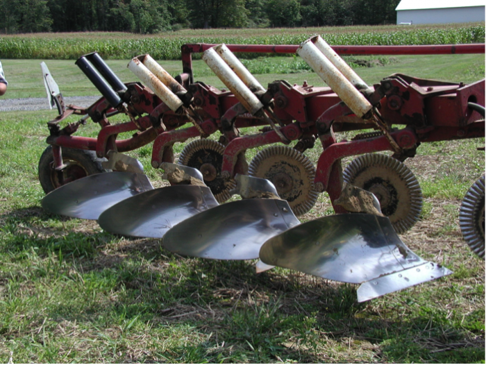
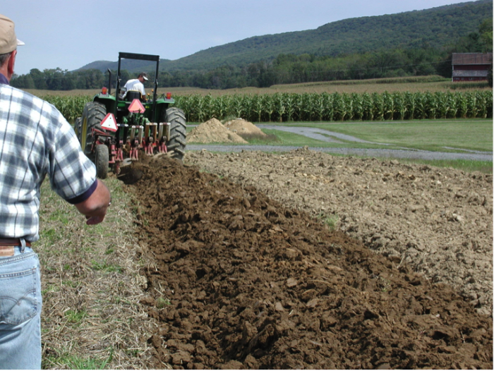
In conventional tillage systems, primary tillage equipment such as the moldboard plow or a rototiller inverts the soil. A second tillage event or plow is often used afterward to break up large soil clods into smaller particles, with the goal of improving seed to soil contact. See photos below.
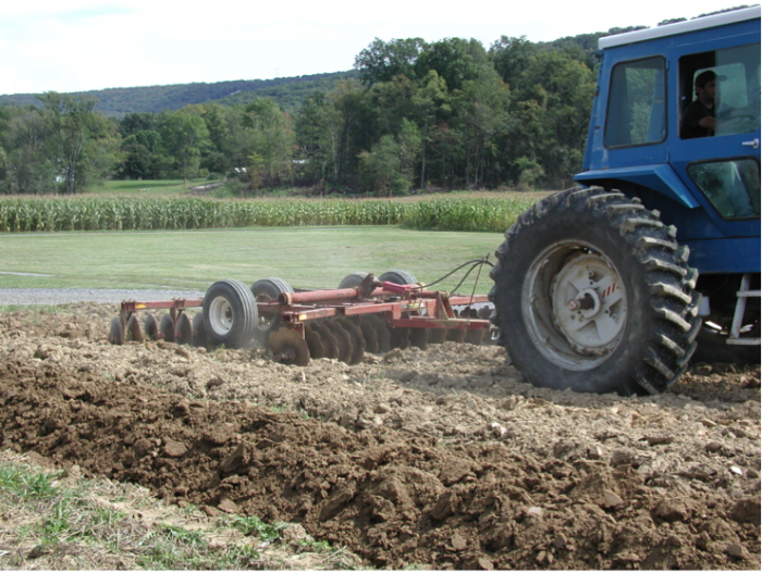
Removing or mixing-in crop residue leaves the soil exposed and prone to wind and water erosion, as well as soil moisture loss. Tilling crop residue into the soil also makes residues more accessible to soil organisms and incorporates oxygen into the soil, increasing the decomposition rate of the residues and decreasing organic matter content at the soil surface and plow layers. Tillage also disrupts soil organisms, particularly mycorrhizal fungi, and soil physical properties such as water stable aggregates.
Conservation tillage or minimum tillage is another soil preparation method designed to reduce soil erosion by reducing disturbance and leaving some plant residue (at least 30%) on the surface. The soil is not inverted, but the surface is disturbed and often a high proportion of crop residues are mixed in with tillage equipment such as a disk plow or a chisel plow.
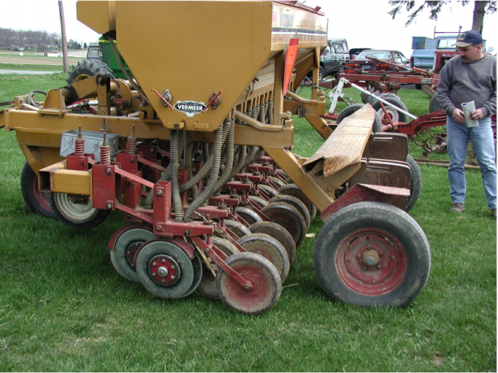
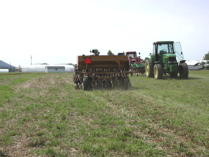
No-till or Direct-seeding is designed to eliminate tillage, by cutting a slit in the surface and placing the seed in the slit. In addition to minimizing crop residue disturbance, the crop is planted in one pass across the field, thereby reducing erosion, labor, and fuel needed to prepare a field and plant the crop.
Some hurdles to no-till adoption As discussed earlier, there are a number of reasons that farmers till the soil. For instance, conventional tillage can terminate perennials, cover crops, and weeds prior to planting the subsequent crop. Without conventional tillage, farmers typically use herbicides to terminate the previous perennial or cover crop and control weeds. In cool environments, crop residues can harbor pathogen and insect pests, and insulate soil, which can slow soil warming in spring and delay crop emergence. These factors can reduce crop yield, particularly if farmers don't rotate crops to interrupt pest life cycles. In addition, although farmers typically need less tillage equipment to plant with no-till, there is an initial cost associated with purchasing no-till equipment for farmers who use conventional or conservation tillage equipment. And with new equipment, farmers need to learn how to adjust no-till planters to ensure that seed is planted at the optimal depth. Consequently, no-till planters are typically heavier to cut through crop residues and place seeds at a sufficient depth for good seed to soil contact.
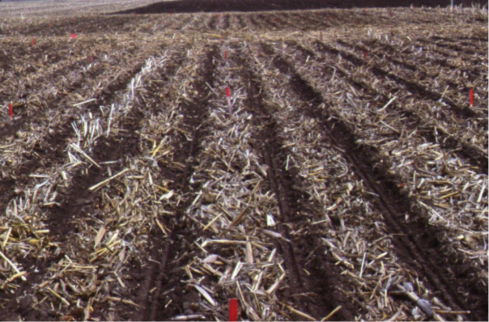
Zone or strip tillage When soils have high crop residue and/or are high in organic matter, or are not well-drained, soils can remain cool and delay seed germination. Zone tillage or strip tillage incorporates the insulating crop residue in a narrow zone or strip of soil where the seed is placed. Residue between the seed planting zones is not disturbed or removed. Removing the soil insulating layer increases the rate of soil drying and warming in close proximity to the seed, promoting earlier seed germination compared to soil with residue left intact.
Reading
Read more about tillage and how it impacts soil, in Chapter 16 (Reducing Tillage) of Building Soils for Better Crops [6].
Continuous Cover Through Crop Management
Continuous Cover Through Crop Management
Soil conservation practices are most effective when they reduce soil disturbance or tillage and also maintain live plants in the soil.
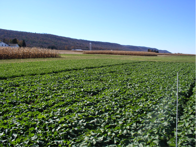
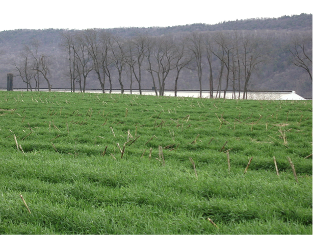
As discussed in Module 5, perennials provide year-round live plant cover that protects soil from erosion; and their live and large root systems support rhizosphere activity and return organic matter to the soil all year. To provide continuous live roots for soil conservation and soil health, perennial crops can be rotated with annual crops, and double crops and cover crops can be integrated into annual cropping systems. Recall that in Module 7.1, a dairy crop rotation of corn-alfalfa was shown in Fig. 7.1.3b, and double cropping in Fig.7.1.4. The photos below also illustrate examples of how year-round cropping provides multiple agroecosystem benefits.
In addition, consider how managing crops and soils for soil conservation and health can enhance agricultural resilience and adaption to climate change. For instance, by increasing soil organic matter content, agricultural soil can: i. contribute to carbon sequestration (removing carbon dioxide from the atmosphere and storing it in soil), ii. improve soil structure and porosity and enhance water infiltration and water content in soil, and iii. store and cycle nutrients. Perennial crop production and double-cropping can utilize potentially longer growing seasons; provide more year-round protection of soil from erosion, and planting and harvesting crops at multiple times of the year can reduce the risk of extreme weather events or irregular weather interfering with cropping activities.
For more discussion of a crop-soil system management approach, watch the three short videos below from NRCS about the benefits of cover crops on soil health.
-
Video: The Science of Soil Health: Using Cover Crops to Soak up Nutrients for the Next Crop USDA NRCS [7] (3:08)
Click for a transcript of the using crops to soak up nutrients video.Interviewer: No farmer wants to lose precious nutrients in the cool season, but this is exactly what happens when a field is left fallow. We've visited with Penn State's Dr. Sjoerd Duiker to talk about how they use cover crops to ensure that those nutrients stay where they belong. Sjoerd: You know in Pennsylvania a special characteristic of our state is that we are very heavily reliant on the dairy sector. And our farms, they spread manure, and they spread it at times when there might not be living vegetation in the field. So the water-soluble portion of the nutrients can easily be lost. And we, being a large part of our state is in the Chesapeake Bay watershed, so we are under scrutiny. There's a lot of concern about nutrient losses to the rivers, to the streams, and eventually to the Chesapeake Bay. There are basically two periods during the year that we lose a lot of nutrients. One is in the fall, there's a little peak. And then most of the, especially nitrogen loss, occurs in the spring. That time, April, May, when we come out of the winter. The soil starts to thaw, the soil is saturated, mineralization is taking place, and now we get leaching through the soil profile. A lot of nitrogen is then lost through groundwater and eventually then, through lateral flow, ends up in the streams. So what we are trying to do is to have living cover crops that take up all those nutrients, the water-soluble nutrients, nitrogen primarily, is made available and is then absorbed by the roots. It's like a sponge, a continuous sponge, that is there. We have evaluated the nutrient uptake and what we can find in the above-ground biomass, depending on growing conditions and the type of cover crop, but it can be even 200 pounds of nitrogen per acre into the above-ground vegetation only. So that makes up typically perhaps 80 percent of the total plant biomass. The rest is underground. All that would otherwise have been liable to loss. So what we are normally considering when we grow a full corn crop, we might assume that that corn crop needs 150 pounds of nitrogen, perhaps 200 pounds of nitrogen per acre. So we are trying to really stimulate that cycling of those nutrients and avoiding them from being lost from the system. We would like to see every acre of corn silage in the state be followed with cover crops, no more fallow after corn silage. -
Video: The Science of Soil Health: Without Carrot or Stick USDA NRCS [8] (2:39)
Click for a transcript of the without carrot or stick video.Interviewer: Planting cover crops enhance the soils ability to function as a nutrient recycler. Penn State's Dr. Sjoerd Duiker talks about how dairy farmers in his state are using cover crops to improve their businesses, without regulations or subsidies. Sjoerd: In my work, I have concentrated on helping farmers adopt no-tillage systems, diversify their crop rotations, and also to fill any fallow periods in the crop rotation with living vegetation. So our principles, our guiding philosophy, is basically to have a living vegetation and living roots systems in the soil 365 days a year. So I have a project that is actually called, without carrot or stick. Because we are trying to stimulate the farmers to adopt cover crops without a carrot of subsidies, without a stick of regulation. Usually, we have 10 dairy farmers all over Pennsylvania, and it is all focused on cover crops after corn silage. There is a good window for planting the cover crops and there is a good also opportunity for using the cover crops for forage. Instead of them buying feed from outside, they are cycling more nutrients on their own farm. It's going through the animal, they’re producing some products, they’re producing manure, the manure goes back on the field. If we can produce more feed on our own farm, and cycle more nutrients on our own farms, it is very beneficial. Interviewer: How's that make you feel? Sjoerd: Yeah, that is very satisfying. We've already seen an enormous increase in the adoption of no-tillage. But now we want to really emphasize, as part of that no-till system, we need to fill all those fallow periods with living crops. And so the cover crops are a big part of that and we see that now our farmers are actually starting to use those practices. So we think it will be very beneficial for soil quality, for nutrient management, the nutrient cycling. And the farmers are intensifying their production, so we hope they can produce more forage on their own farms, cycle more nutrients on their own farm. -
Video: The Science of Soil Health: Cover Crops and Moisture USDA NRCS [9] (3:26)
Click for a transcript of the cover crops and moisture video.No cropping system is drought proof, but there are things that farmers can do to mitigate the effects of a dry year. The road took us to NC State's Dr. Chris Reberg-Horton to discuss how cover crops affect water dynamics. Chris: Water, I think, is going to be real limiting factors over the next several decades and particularly here in the southeast. We tend to get most of our summer precipitation and these huge rain events. And one of the things that cover crops bring to the system is they slow the movement of water across our fields, and so we think that we have a lot of yield potential that we can garner from cover crop residues by allowing more water to soak into the soil Interviewer: Okay, okay. Well, tell us about some of the actual work that you've done. Chris: Sure, well we've worked both in corn and soybeans at this point. So we started with soybeans and there we use a rye cover crop. One of the ways that we're going to get more biomass into these systems is not treating the cover crop as an afterthought, thinking of it as a key part of the production philosophy of the field. We plant our rye cover crops early, which makes a big difference. We try to plant that in October, as opposed to throwing it in, you know, November December timeframe. That does tremendous amounts for us. It's interesting what that does for water dynamics. I think for one thing it makes it actually drier in the spring. If you think about it, if you're gonna plant a plant out there over the winter and we're going to grow it, we're gonna extract water out of the soil over the season. So as you plant, we can actually be a fair bit drier than we would be. Now that can be a plus or minus, depending on where you're farming. So in some areas, your traditional no-till agriculture without the cover crop, we can be a bit wet and cool later into the spring. And so getting into the field can be troublesome. Some drying can be a benefit on some soil types. On some soil types, it can be a greater concern. But then at some point in the season of that soybean, we then flop. The plot that had the cover crop now becomes the wetter one because we're soaking in. Again, those big rain events that come in, we're allowing greater water infiltration in those than we are in a conventional no-till setting where we don't have that residue to break up the water. Corn, of course, we stand even greater benefit. In our work with corn we've done, again, that side-by-side comparison, with and without the cover crop. And we can see that certainly by the time we get to silking, which can be a very important time for water dynamics, those two have flopped under our conditions. So now the one with the cover crop mulch is now wetter than the one without a cover crop mulch. Both of them done via no-till. We can actually score that. We go in and we look at our corn plots and we rate when in the morning, under drought conditions, does the leaf first start to curl. That's a powerful integrator, telling you what the water stress on that plant is. And the plants under normal no-till are rolling well before, hours before we see them rolling under a no-till with a massive cover crop under there. So we think that alone right there, gives you a longer period each day to grow the set carbohydrates, to build your yield.
Check Your Understanding
Describe two or three practices that are components of the conservation system or agroecological approach of soil conservation and health.
Click for the answer.
Reduced soil disturbance through reduced tillage, particularly no-till or zone/strip tillage; Continuous plant cover through the integration of perennials, double crops, and cover crops. Returning organic matter to the soil through the application of animal manure, compost, and the integration of green manure and cover crops that are returned to the soil.
Conservation Agriculture in Brazil Case Study
Conservation Agriculture in Brazil Case Study
Activate Your Learning
Go to the FAO UN website and read their brief description of Conservation Agriculture. Then watch the short video “Conservation Agriculture in Southern Brazil [10]” (4:41).
PRESENTER: In Santa Catarina and Piranha, southern Brazil, severe soil degradation over the past two decades left many farmers with no choice-- find a solution or abandon the land. Roland Ristow began experimenting with no-tillage farming more than 20 years ago. He is considered a pioneer of conservation agriculture.
ROLAND RISTOW: [NON-ENGLISH SPEECH]
INTERPRETER: Before starting conservation agriculture, there was a lot of work to do-- plowing harrowing, tilling. And then erosion would carry off all the water. If we hadn't changed over, all these would be desert now, and there would be no crops, just stones.
PRESENTER: Cover crops are the key. Grown between annual crops, they protect the soil from the damaging effects of heavy rainfall, sun, and wind, provide nutrients, and facilitate water infiltration by reducing soil compaction. By integrating livestock production, Francisco Sedosvki saves money on feed and effectively lets the cows prepare the land for direct seeding of his next crop.
His integrated approach to resource management, which includes pig raising and fish farming, actually improves the quality of the local water supply. This farm is a model of environmentally-friendly recycling.
FRANCISCO SEDOSVKI: [NON-ENGLISH SPEECH]
INTERPRETER: We don't have to worry now because we have clean water on our farm. There's no animal waste in our stream. The situation has really improved. We can raise pigs without damaging the environment.
PRESENTER: Direct seeding makes conservation agriculture considerably less labor-intensive than conventional farming and more cost-effective. The elimination of tillage reduces machinery and fuel costs, while cover crops reduce the need for expensive chemical inputs. And even in dry years, yields increase as soil quality and water infiltration improves.
DERLI BOITA: [NON-ENGLISH SPEECH]
INTERPRETER: With conservation agriculture, you save money and you can produce more. I don't know the exact figures, but I think that our production has increased by about 30% or 40%.
PRESENTER: Time saved with conservation agriculture is used by farmers to diversify production and supplement their income. Products like sugar and jam can be sold all year round to ensure financial security for small-scale farmers. In southern Brazil, conservation agriculture has made sustainability a reality, and the Food and Agriculture Organization is already promoting the same approach in Africa and Central Asia.
JOSE BENITES: [NON-ENGLISH SPEECH]
INTERPRETER: I think that conservation agriculture really could solve a food security problem, and it could also be a valuable weapon in the fight against poverty.
PRESENTER: For many families in southern Brazil, that fight has already been won by making the most of natural resources and letting nature take its course.
After Watching the Video, Answer the Following Three Questions:
Question 1 - Short answer
Describe the soil and crop management practices that the video about Conservation Agriculture describes that promote soil quality and crop productivity.
Click for answer.
i. No-till farming, ii. Cover crops that protect the soil from erosion, provide nutrients, and reduce soil compaction, iii. Integrating livestock and crop production.
Question 2 - Short answer
In Brazil, what were some of the ecological benefits of conservation agriculture?
Click for answer.
i. Soil is protected and conserved, ii. Soil quality has improved, iii. Cover crop roots reduce soil compaction and improve water infiltration into the soil, iii. Integrating livestock and crop production helps recycle nutrients, and with fish-farming, there is less animal waste in the stream.
Question 3 - Short answer
In Brazil, what were some of the socio-economic benefits of conservation agriculture?
Click for answer.
i. No-till or direct-seeding saves labor and time to plant crops, reduces machinery needs and saves money, ii. With reduced tillage and cover crops, farmers need fewer inputs, have saved money, and production has increased, iii. Time saved has allowed farmers to diversify production and produce added-value products.
Summary and Final Tasks
Summary
In this module, you have learned how crop and soil management can protect soil from erosion, improve soil quality and maintain crop productivity in the long-term. Recall that these crop and soil conservation management practices can also help agriculture adapt to climate change because soil that is high in organic matter can store more carbon, nutrients, and water. In addition, diversifying cropping systems can reduce the risk of weather impacting all of the crops on a farm and region, and utilizing a diversity of seasonal crops and varieties can take advantage of longer or potentially different growing seasons.
Reminder - Complete all of the Lesson 7 tasks!
You have reached the end of Module 7. Double-check the to-do list on the Module 7 Roadmap [12] to make sure you have completed all of the activities listed there before you begin Module 8.1.
References and Further Reading
Erosion Control Measures for Cropland: University of Nebraska Plant and Soil ELibrary http://passel.unl.edu/pages/printinformationmodule.php?idinformationmodule=1088801071 [13]
Karlen, D.L., M.J. Mausbach, J.W. Doran, R.G. Cline, R.F. Harris, and G.E. Schuman. 1997. Soil quality: A concept, definition, and framework for evaluation. Soil Sci. Soc. Am. J. 61:4-10.
Magdoff, F. and H. VanEs. 2009. Building Soils for Better Crops. Edition 3. Chapters on Cover Crops, Crop Rotation and more. Sustainable Agriculture Network, USDA. Beltsville, MD.
Module 8: Pests and Integrated Pest Management
Module 8: Pests and Integrated Pest Management
Introduction
Agroecosystems have many beneficial species that play important roles in processes such as nutrient cycling, pollination, and pest suppression; but some species, typically called pests, reduce crop or livestock yields and/or quality. This module introduces three types of agricultural pests (insects, weeds, and pathogens) and some of the scientific research, technologies, and management approaches developed to reduce agricultural pest damage.
Goals and Learning Objectives
Goals and Learning Objectives
Goals
- Learn some benefits of insects, some characteristics of insect and weed pests, some challenges associated with insect and weed pest control, and how trophic interactions can contribute to insect pest control
- Learn what IPM is and how to apply the economic threshold concept to interpret if a pest population has reached an economic threshold
- Learn some transgenic pest management technologies and their impact
- Understand how few pest control tactics can select for pest resistance while integrated pest and weed management can contribute to long-term successful weed and pest management
Learning Objectives
After completing this module, students will be able to:
- Describe characteristics of insect pests and factors that make them successful pests, as well as beneficial characteristics of insects.
- Explain some history of agricultural pesticides.
- Describe factors that contribute to pests evolving resistance to pest control strategies.
- Discuss what IPM is and why it is effective.
- Interpret how to apply pest scouting data and distinguish if pests have reached an economic threshold.
- Analyze pest management scenarios and describe the agroecosystem benefits of IPM.
- Describe and compare the characteristics of natural ecosystems and agroecosystems, and explain how trophic level interactions and biodiversity may contribute to pest control.
- Describe characteristics of weed pests and factors that make them successful pests.
- Describe categories of weed management tactics with examples of weed control practices.
- Explain what organisms and factors contribute to crop diseases.
- Explain some recent transgenic pest management technologies and analyze and interpret scientific data about transgenic technologies.
- Differentiate pest control approaches that are likely to be effective in the long term based on IPM principles, and generate or formulate IPM approaches to enhance pest control.
Assignments
Module 8 Assignments Roadmap
Detailed instructions for completing the Summative Assessment will be provided in each module.
| Action | Assignment | Location |
|---|---|---|
| To Read |
|
|
| To Do |
|
|
Questions?
If you prefer to use email:
If you have any questions, please send them through Canvas e-mail. We will check daily to respond. If your question is one that is relevant to the entire class, we may respond to the entire class rather than individually.
If you prefer to use the discussion forums:
If you have any questions, please post them to the discussion forum in Canvas. We will check that discussion forum daily to respond. While you are there, feel free to post your own responses if you, too, are able to help out a classmate.
Module 8.1: Insects and Integrated Pest Management
Module 8.1: Insects and Integrated Pest Management
Ecosystems have many trophic levels of organisms including primary producers, herbivores, omnivores, carnivores; parasites, and decomposers. Agroecosystems are ecosystems managed for food and fiber production that have less diversity and typically fewer trophic interactions than natural ecosystems. But diverse organisms and their trophic interactions provide important functions in agroecosystems including, for instance, decomposition and nutrient cycling; plant pollination, and pest suppression. Organisms that reduce agricultural productivity and quality and are referred to as agricultural pests; these include weed pathogens, insects, and other herbivorous organisms. Mammals that graze or browse crops (ex. deer and rodents), and other arthropod species such as mites and slugs (mollusks), can also reduce crop yields through grazing and seed predation.
Natural Ecosystem and Agroecosystem Comparison
Natural Ecosystem and Agroecosystem Comparison
Pest species can be present in agroecosystems, but not cause significant crop yield loss or livestock productivity reductions. Why? What factors prevent pest populations from reducing yield? One explanation may be that the crop or livestock is resistant to the pest. For instance, a crop plant may produce compounds that fend off pathogen infection or deter insect feeding. And if environmental conditions and resources are ideal, the plant may be able to grow and recover from pest infestation. What other ecological processes and factors might contribute to agricultural resilience to pests or other stresses such as climate change?
Activate Your Learning
Question 1 - Short Answer
Draw a food web pyramid and label the trophic levels as categories of organisms with i. primary producers at the bottom, ii. herbivores next, ii. omnivores and carnivores at the top of the pyramid. Chose a natural ecosystem and list all of the species you can think of that are found at each trophic level in the natural ecosystem. Then draw a second food web pyramid for a type of farm that you are familiar with, and list all of the species you might find at each trophic level. Describe how the natural ecosystem and the agroecosystem compare. How do they differ?
Click for the answer.
You should have many more species at each trophic level in the natural ecosystem. Additionally, the genetic diversity within species in the natural ecosystem is typically greater than in the agroecosystem.
Question 2 - Short Answer
Odum (1997), an Ecologist summarized some of the major functional differences between natural and agroecosystems that are shown in the table below. Consider how your natural and agroecosystem food pyramids offer examples of the below ecosystem differences. How many predatory and parasitic species are there in the natural ecosystem and agroecosystem? How might the presence of predatory and parasitic organisms impact agricultural pests? How might genetic diversity contribute to pest management and ecosystem stability?
Click for the answer.
Although you may not be familiar with parasitic species such as wasps and nematodes, you likely can think of many predatory species: humans, large and small mammals, predatory birds, rodents, fish, and arthropods (ex. beetles, spiders, ants, etc.)
In natural ecosystems there tend to be more niches and a higher diversity of species compared to most managed agroecosystems that are simpler, have fewer predatory and parasitic species, and less genetic diversity within a species. As the table below indicates with fewer trophic interactions, there are fewer species to reduce pest populations and prevent them from reducing agricultural yield and quality. Further, with low genetic diversity within agricultural species and across the landscape, the agricultural system is more vulnerable to pest outbreaks than natural ecosystems.
| Property | Natural Ecosystem | Agroecosystems |
|---|---|---|
| Human Control | Low | High |
| Net Productivity | Medium | High |
| Species and Genetic Diversity | High | Low |
| Trophic Interactions | Complex | Simple, Linear |
| Habitat Heterogeneity | Complex | Simple |
| Nutrient Cycles | Closed | Open |
| Stability (resilience) | High | Low |
Insects
Insects
Insects are the most diverse group of animals that are found in most environments. In the Animal kingdom, Insects are in the Phylum Arthropoda; Arthropods have an exoskeleton of chitin that they shed as they grow; they also have segmented bodies and jointed appendages. In addition to the Class Insecta, the Arthropoda also includes the arachnids (spiders and mites), myriapods (ex. centipedes), and crustaceans (crabs, lobsters, etc.). Insects are distinguished from the other Arthropod classes by the following features:
-
As adults and in some species in the juvenile stages, insects have three body parts: the head, thorax, and abdomen. Although in some insect species, some of the three body parts are fused together and may be difficult to distinguish. See this website for images and more discussion of insect anatomy: Purdue University, College of Agriculture, Department of Entomology, 4-H and Youth: Insect Anatomy [21]
- The adults have antennae on their heads that they use to sense their environment, and they have three pairs of legs or six legs.
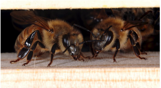 Figure 8.1.1: Honeybees are important pollinator insects. Note the three body parts (head, thorax, and abdomen) two antennae, and three pairs of legs.Credit: MaryAnn Frazier, Department of Entomology, Penn State University [22]
 - Most insects undergo a morphological change that occurs between the time they hatch from eggs and develop into adults. The morphological change is called either complete metamorphosis or incomplete metamorphosis referring to how significantly the insect's appearance changes from the early stage of development to the adult stage. Go to these links to see images of the types of metamorphosis and read more about insect metamorphosis: ASU School of Life Sciences: Metamorphosis [23]
Check Your Understanding
Question - Multiple Select
Browse the following websites for two major agricultural crop pests. What kind of organisms are they? In what stage of their lifecycle do they cause the most damage to the crop plants?
Click for answer.
Both are insects that undergo complete metamorphosis. They do the most crop feeding and damage in the larval stages when they resemble worms, that are sometimes also called caterpillars. Thus, their common names include the name: worm.
Feeding Types
Insects may be herbivores or omnivores. Herbivorous insects may eat plants by directly feeding on plant tissues such as leaves or roots. Herbivorous insects include caterpillars, beetles, grasshoppers, and ants. Some insects pierce plants and suck plant nutrients from the plant vascular system, typically the phloem, (the cells that transport plant carbohydrates and amino acids); although some insects feed on the xylem, the vascular cells that transport water and nutrients. Examples of piercing-sucking insects include aphids and mosquitoes. By contrast, butterflies and moths have siphoning mouthparts for drinking nectar. Omnivore insects consume multiple kinds of food including other insect prey and plant tissues such as leaves and/or nectar and pollen.
Beneficial insects
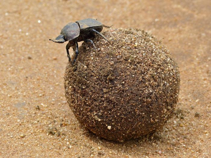
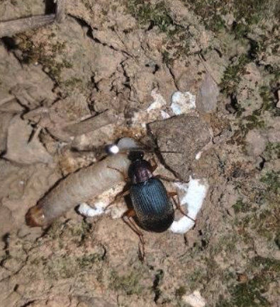
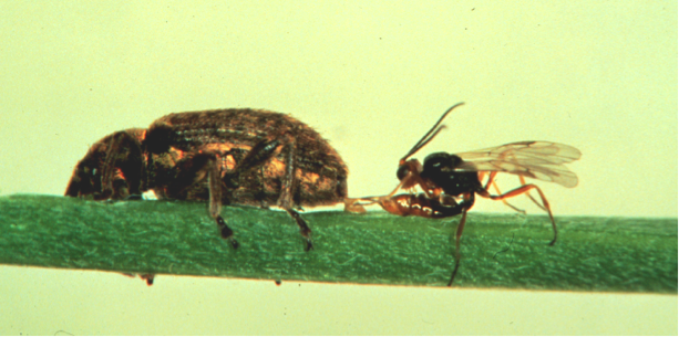
Although insect pests are major agronomic pests, only about 1% of insect species are agricultural pests. Insects also contribute to important ecosystem processes, including: i. pollination, ii. predation and parasitism (ex. lady beetles, lacewings, praying mantis, parasitic wasps); iii. decomposition of organic materials such as crop residues and manure (Ex. dung beetles) iv. providing food for other organisms, such as fish and birds. Review the photos below for some categories of beneficial insects, and some of their characteristics here: National Pesticide Information Center [26]
Activate Your Learning
Read the following website: Omnivorous Insects: Evolution and Ecology in Natural Agriculture Ecosystems [29].
Then answer the following questions:
What did scientists observe happened to cotton plants and insect herbivores after cotton plants were injured by herbivorous insects?
Click for answer.
To conserve or maintain predatory insects, what is required? What can farmers do to attract and conserve predatory insects?
Click for answer.
Pest Management
Pest Management
Humans have developed methods of insect and pest control for centuries.
Reading
Read the following brief history of pesticides and then answer the questions that follow:
Pesticide Development: A Brief Look at the History [30]. Taylor, R. L., A. G. Holley and M. Kirk. March 2007. Southern Regional Extension Forestry. A Regional Peer-Reviewed Publication SREF-FM-010 (Also published as Texas A & M Publication 805-124)
Check Your Understanding - Pesticide Development: Brief History
What chemicals were used to control pests from 1700 to the early 1900s?
Click for answer.
When was DDT invented and what was it first used for?
Click for the answer.
When and why was DDT banned?
Click for the answer.
Pesticide Resistance
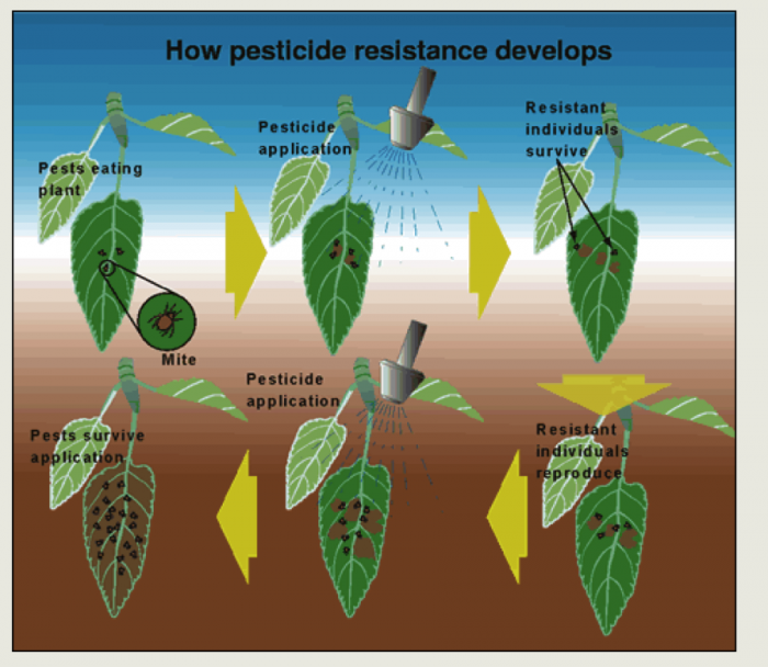
Soon after the development of DDT in 1939 and the dawn of the modern insecticide era in the 1940s, scientists began to understand that pesticides were not the silver bullet of pest control. Particularly when a pesticide or one effective pest control strategy is relied on, the control tactic acts as a strong selective force for the development of resistance to the tactic in the target pest population. With the continuous application of the same pesticide, individuals that are susceptible to the pesticide are killed, leaving the few resistant individuals that survive to reproduce a offspring that are resistant to the pesticide. See the figure below for an illustration of how frequent reliance on one insecticide can select for a resistant insect population. Further, since many early pesticides were broad spectrum pesticides, the natural enemies of agricultural pest populations were also destroyed, contributing to pest population outbreaks.
In 1984, the US Board of Agriculture of the National Academy of Sciences organized a committee to explore the science of pest resistance and strategies to address the challenge. A report called "Pesticide Resistance: Strategies and Tactics for Management" was co-authored by the Committee on Strategies for the Management of Pesticide Resistant Pest Populations and published in 1986 by the National Academies Press, Washington D.C. In Chapter 1, G. P. Georghiou (1986) documented the development of pest resistance across multiple pest organisms (see pages 17 and 28 for figure 2 [32] and figure 8 [33]), as well as how difficult and costly it was becoming to develop cost-effective pesticides (see figures 12 and 13 [34] on page 36).
In the report, the Committee recommended using Integrated Pest Management or IPM to reduce the evolution of pesticide resistance and provide more long-term, effective pest control. As early as 1959, a team of scientists (Stern et al.) in California had also proposed that pest control that integrated both biological and chemical control approaches, was needed to prevent pest resistance to pesticides and pest control. Stern et al. (1959) defined terms and concepts that are fundamental to IPM today.
Understanding Economic Thresholds
Understanding Economic Thresholds
Read the following two fact sheets for a description of Integrated Pest Management and the terms that Stern and his colleagues defined in 1959, which are still used today (economic injury level, economic threshold, and general equilibrium position). Then watch the following short video and answer the questions below:
-
The Integrated Pest Management (IPM) Concept [16]. D. G. Alston. July 2011. IPM 014-11. Utah State University Extension and Utah Plant Pest Diagnostic Laboratory
- IPM Pest Management Decision-Making: The Economic-Injury Level Concept [17]. D. G. Alston. July 2011. IPM 016-11. Utah State University Extension and Utah Plant Pest Diagnostic Laboratory
Activate Your Learning: IPM Concept and Decision-Making
Describe three things that are integrated into IPM.
Click for the answer.
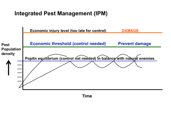
On the IPM figure below, which IPM pest population terms from the article could describe the lines labeled A, B, and C?
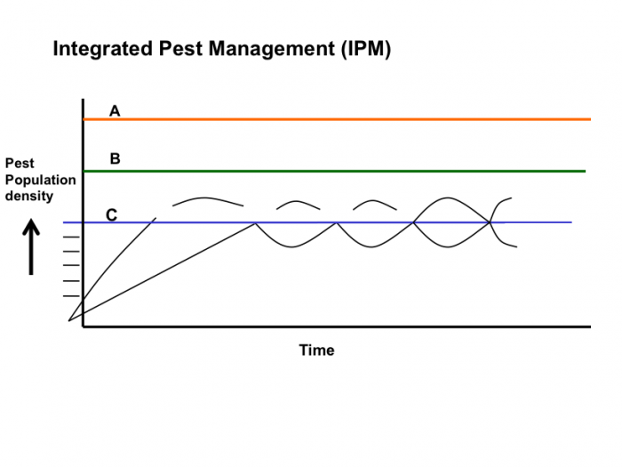
Click for the answer.
How would you describe the damage that the pest had caused to the crop at each of these pest population densities?
Click for the answer.
Watch the first 4.11 minutes of the below video: Integrated Pest Management (IPM) in Apple Orchards, which describes European Red Mite pests and predatory mites in Pennsylvania apple orchards.
Video: Integrated Pest Management (IPM) in Apple Orchards [35] (8.34)
What are the potential benefits of scouting for the European red mites and predatory mites in Pennsylvania orchards?
Click for the answer.
Formative Assessment: Australian Grain Crop IPM and Determining the Economic Threshold of Potato Leafhoppers in Alfalfa
Formative Assessment: Australian Grain Crop IPM and Determining the Economic Threshold of Potato Leafhoppers in Alfalfa
Part 1: Australian grain crop IPM
Watch the following video that explains IPM adoption in grain crops in Australia; then answer this question:
1. Identify and explain three benefits of utilizing IPM discussed in the Australian video from the GRDC.
Video 1: GCTV2: Integrated Pest Management (5:46)
Narrator: Now another aspect of the overall push for improved farming practices, is how we control pests; and Jane Drinkwater reports on the latest approach to pest control while looking after the environment.
Jane Drinkwater: Australia's crop production systems are forever improving. A prime example is how we manage insect pests. Where once broad-spectrum, often highly toxic, insecticides were used to blanket eradicate insects, there's a move towards a more holistic approach, and with good reason. Integrated pest management, or IPM, presents a win-win, less damage to the environment and to your hip pocket.
Rowan Peel (Mount Pollock VIC: I love the environment and I want to look after the environment, but I have to make a living. IPM has given us the opportunity to do all of these things, both look after the environment and to make more money.
Jane: IPM uses multiple strategies to manage insect pests. One of the tactics is to let an army of the insects’ natural predators, or beneficials, fight the battle for you, and that means holding off on the use of broad-spectrum chemicals.
Rowan: I've probably learned that nature has its way of handling things its own way. You just have to give those beneficials that time. And when you understand that when you are using a broad-spectrum insecticide that you might control it straight away, but you'll get another flight straight in. But you've killed all your beneficials, and you've killed beneficials for other pests later on. And some of these beneficials don't have the lifecycle of an aphid. You know, their lifecycle might be only once or twice a year. And so you know, economically, if you look at the long-term, you're a long way worse off.
Jane: For insects without natural predators, or where the ratio of pests to beneficials is high enough to affect yield, strategies include the application of pesticides to problem areas only and the use of chemicals which target the problem pests, without damaging the beneficial insects. Rowan: We actually treat the seed for earwig infestation to give ita protection. But if there is a further problem, and that may well only be in certain areas of the paddock, which we tend to know where they will be, we will make up a brew of wheat, a little lawsben, and a little bit of vegetable oil. And we'll go out and spread just on that area. So as the earwigs are attracted to that bait, rather than all the other insects.
Jane: Peter Enkelmann’s been using IBM for more than a decade. While his beneficials successfully control silver leaf whitefly, there are still a few pests without natural predators.
Peter Enkelmann (“Riverview” Byee QLD): The chemistry that we use here, it takes out the beneficial insects. So the attitude is to delay spraying any product at all basically, apart from very few natural viruses, right through until the very last.
Jane: And using IPM means, when you do need to pull out the big guns, they're more likely to work.
Peter: One of the big advantages is that resistance to our traditional chemistry is just dropped dramatically.
Jane: But how do growers know when to take action? Well thanks to research funded by GRDC, entomologists have data on the density of pests in each crop that will lead to economic damage. Growers measure the number of pests in their fields and only take action once they've reached this threshold.
Hugh Brier (Senior Entomologist, Primary Industries and Fisheries, DEEDI QLD): So the short-term gain is you might avoid unnecessary sprays. Another short-term gain is by not spraying when you didn't need to, you might avoid flaring another pest which is more expensive to control, so that's another benefit. Longer term, if you avoid spraying unnecessarily, you build up beneficials in the whole system and the system is much more stable.
Jane: Fundamental to successful integrated pest management is the ability to correctly identify pests and beneficial species, and to regularly monitor both populations.
Hugh: In row crops, we use a bed sheet. So we'll go and we shake the plants from meter of row and that shakes all the insects out, or a lot of them out onto the bed sheet and you can count them.
Jane: With IPM leading to lower costs and better environmental outcomes, GRDC views it as an important step forward. Apart from funding IPM Research, GRDC also provides information and training for growers.
David Shannon (GRDC Southern Region Panel Chairman): We have run a series of workshops, IPM workshops. We also work with the grower groups so that grower groups can scale up their grower members on the use of IPM.
Jane: And it's well worth getting up to speed.
Rowan: I find the system of IPM very easy because it's not an almost do nothing, but you just don't worry about it anywhere near as much.
Jane: With IBM's effectiveness in controlling insects, while reducing costs both financial and environmental, it's here to stay.
Rowan: IPM for us has cut down our chemical usage, insecticide usage a long way and you feel better for not using it.
If the video does not load for you, go to GCTV2: Integrated Pest Management [36]
Part 2: Determining the Economic Threshold of Potato Leafhoppers in Alfalfa
Read the Penn State University Potato Leafhopper on Alfalfa Fact Sheet [37].
Scenario
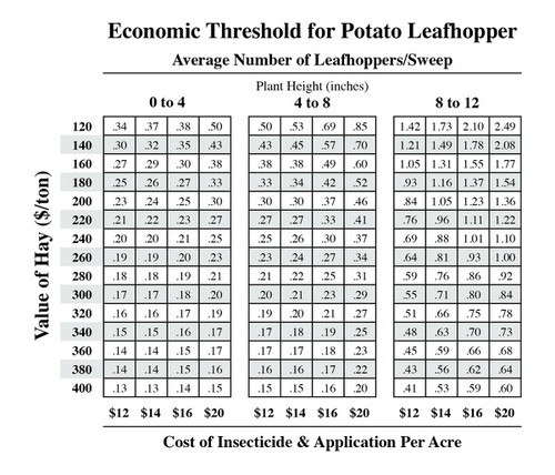
Assume that you followed the procedure described in the Penn State fact sheet to scout for Potato Leafhoppers in an alfalfa field by sweeping 20 times with your sweepnet in each of 5 different locations in the alfalfa field. The number of leafhoppers that you found in the 5 different locations was: 15, 12, 16, 7, 13 when the alfalfa crop was about 11 inches tall. You would like the alfalfa to grow about 25-30 inches height before harvesting it for hay, this could require 2 to 3 more weeks of growth, depending on rainfall. Based on current alfalfa hay prices in your region, you estimate your alfalfa hay is worth about $250/Ton, and the insecticide you would spray to control the leafhoppers would cost about $16/A. If you spray the alfalfa field, it cannot be harvest until 7 days after spraying the insecticide; and due to toxicity to bees, the alfalfa should not be sprayed if it is flowering.
Answer the following questions:
- Calculate the average number of leafhoppers per sweep. Add the number of potato leafhoppers from the 20 sweeps in each of the 5 locations (20 X 5= 100 sweeps). Divide by 100 to calculate the number of leafhoppers per sweep. Use the Economic Threshold Table from the Fact Sheet for Potato Leafhoppers, shown here. Has the insect population reached an economic threshold for your crop at this height?
- Based on the average number of leafhoppers per sweep, what should you do? Why?
- If your crop height was 7 inches tall and you had the same number of leafhoppers per sweep that you calculated here, would your pest management decision change and how?
- Discuss at least two potential benefits of using the economic threshold decision tool rather than spraying as soon as potato leafhoppers were first visible.
Files to Download
Module 8 Formative Assessment Worksheet [38]
Submitting Your Assignment
Please complete the Module 8 Formative Assessment in Canvas.
Module 8.2: Weeds, Transgenic Crops for Pest Management, and Pathogens
Module 8.2: Weeds, Transgenic Crops for Pest Management, and Pathogens
Weeds are a major crop pest that persist in agricultural ecosystems, and significant resources are allocated to studying weeds and developing technologies to control them. What characteristics make weeds such significant pests and how can they be controlled? We will employ the plant lifecycle terms that you learned about in Module 6 to describe weed lifecycles and identify effective weed control practices. We will also explore how the principles of integrated pest management are applied in weed management; and you will learn about transgenic pest control practices that have been widely adopted for insect and weed control; as well as some plant pathogen management principles.
Weeds
Weeds
A weed is a plant that is not wanted or a plant growing in the wrong place. In agricultural systems, weeds tend to be unwanted because they compete with crops for light, water, and/or nutrients, and can reduce crop yield and/or quality, particularly if weeds are permitted to grow and reproduce. Weeds may reduce crop quality through contamination with seeds or plant parts that may be toxic, or of poor nutritional or culinary quality (produce off-flavor compounds). Some weeds may harbor crop insect pests or pathogens; and when weeds have a significant negative impact, they can reduce the economic value of agricultural land. On the other hand, if weeds are not numerous enough to reduce crop yield and quality, weeds can provide some agroecosystem benefits. For instance, weeds can provide:
-
protection from soil erosion
- pollen, nectar, and habitat for beneficial organisms and wildlife
- forage for grazing animals
Competitive Characteristics of Weeds
Weeds tend to be plants that are adaptive and competitive in a range of environmental conditions. They typically have seeds or perennial storage organs that enable them to grow rapidly and produce aboveground canopies that compete with crop plants for light, and root systems that compete for nutrients and water. Annual weed species often grow and mature relatively quickly, producing seeds earlier than crops. To increase survival of their offspring, annual weeds often produce many seeds, and some species produce large seeds. Strategies to control annual weed species target terminating them early, to prevent them from competing with crops and producing seeds.
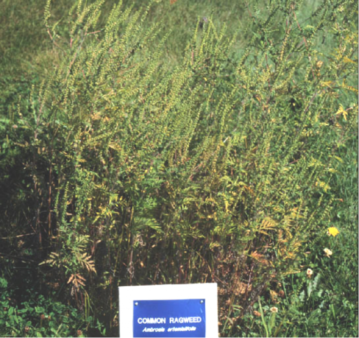
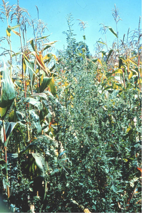
If perennial weeds are growing from the small seeds they produce, they establish more slowly than annual crop seeds. But seeds are not their primary form of reproduction, recall that perennial plants often spread and reproduce via established storage organs such as taproots, tubers, bulbs, and rhizomes (belowground modified stems that store reserves and enable a plant to spread horizontally), or aboveground stolons or storage stem bases. Perennial weeds growing from storage organs can be very competitive with crop plants. If perennial weed storage organs are cut and distributed over a larger area and reburied or partially covered, they can also establish and spread across a larger area. If weed storage organs are left on the soil surface to freeze and thaw over winter or desiccate in mid-summer, then tillage can terminate perennial storage organs. Repeated mowing of plant regrowth may weaken or deplete plant reserves, particularly if it is prior to the end of the growing season when perennials tend to translocate plant reserves to storage organs. Chemical control of perennials is also often most successful at this time when herbicides can be translocated to storage organs.
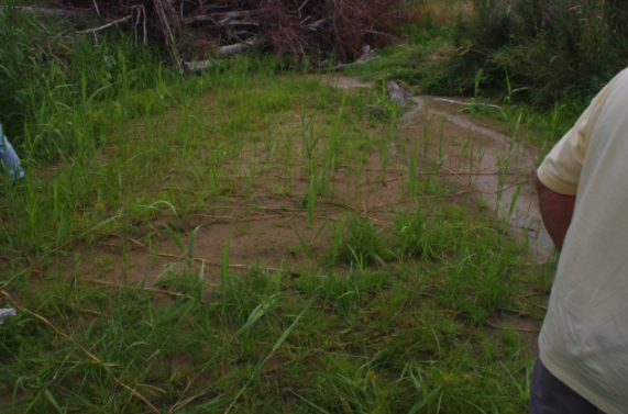
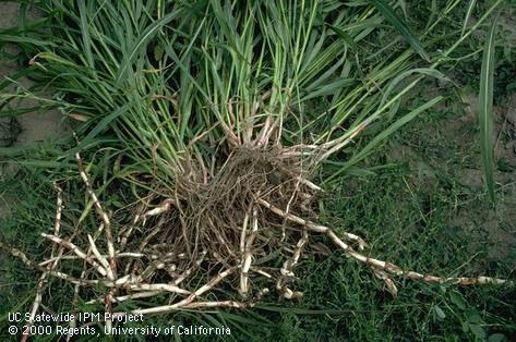
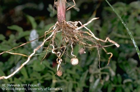
Weed Survival Characteristics
Weed Survival Characteristics
In addition, many weeds have traits that enhance their survival and reproductive success such as: i. hard-seeds or seeds that can remain dormant for long time periods until environmental conditions for germination are good, enhancing weed seed success, ii. plant protective characteristics such as thorns, toxic tissues, protected growing buds, iii. adaptive growth to a wide range of environmental conditions also referred to as plasticity. For example, in a field or lawn that is grazed or mowed to a short height to control weeds, adaptive weeds can produce leaves very close to the soil surface and flowers on short stems below the mowing height.
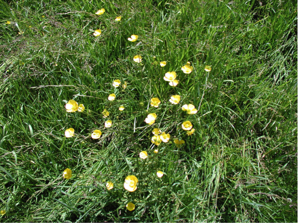
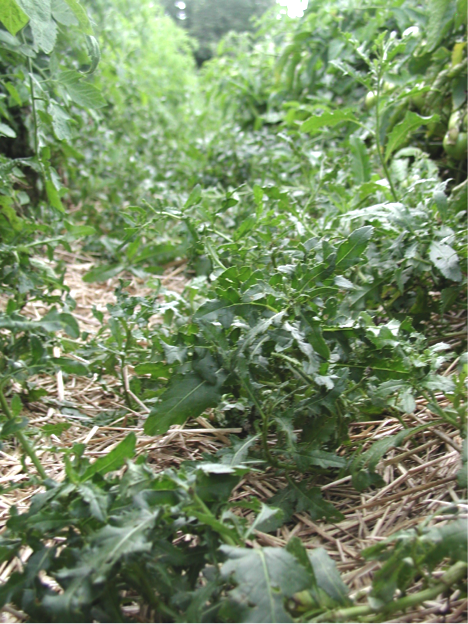
Check Your Understanding
Read about the Velvetleaf weed species (Abutilon theophrasti L.) at Velvetleaf. [42]
Velvetleaf has hard seed. How long can the seed survive? On the website click on the link that discusses Velvetleaf Adaptation and Stress. What examples does the author use to illustrate velvetleaf plasticity or ability to adapt to its growing conditions?
Click for the answer.
Activate Your Learning: Weed Control Practices
Recall what you have learned about crop plant lifecycle classification and characteristics in Module 6.
Read the Australian Department of the Environment website that describes Integrated Weed Management [43]. Click on and read the links that describe each type of weed management technique. After you have read both of the above readings, answer the questions below.
Question 1 - Essay
Review examples of the four weed control strategies discussed in these two online publications. Explain at least two specific weed control strategies that are likely to be effective for controlling annual weeds and explain why they are effective for annual weeds.
Click for the answer.
Annual weeds typically germinate, grow and develop to maturity and seed production quickly, and therefore can offer significant competition with crop plants for light, nutrients, and water. They can also produce seeds and increase weed population pressure relatively quickly. Therefore, annual weeds should be terminated early and especially prior to they produce seeds. Because annual weed species do not allocate significant resources to below ground storage organs, they can be terminated with mechanical or physical control tactics such as: plowing, cultivation, hoeing, removal by hand, hay making, mowing or grazing, soil mulching, and flaming. Allowing weed seeds to germinate and then terminating them with light tillage (stale seedbed) strategically uses tillage for weed control. Annual weed germination and establishment can be suppressed with cultural control practices such as crop rotation, rotating crops with different seasonal life cycles, successive planting (double or triple-cropping); the integration of cover crops; and managing for competitive crops with early crop planting and good crop management practices (competitive crop varieties, soil fertility and health management).
Chemical control with herbicides applied at the recommended time, and rotating or varying herbicide chemistry can reduce the evolution of herbicide-resistant weeds. Biological control can also reduce weed populations and may include conserving habitat for weed seed predators such beetles, small rodents, and birds by integrating cover and perennial crops on a farm, and avoiding pesticides that can reduce weed seed predatory populations. In addition, in some cases, browsing or grazing animals or specific pathogens of weeds such as bacteria or fungi are sometimes introduced.
Question 2 - Essay
Describe at least two weed control strategies that are likely to be effective to control perennial weeds. Explain why.
Click for the answer.
Perennial weeds have below-ground storage organs that they can regrow from (ex. tubers, rhizomes, stolons, and bulbs); therefore mechanical control strategies such as tillage, cultivation, and hoeing can break up and distribute perennial weed storage organs, facilitating the spread of perennial weeds. Mechanical weed control tactics can be effective if they can bring the majority of the storage organ to the soil surface to desiccate or freeze, thaw, desiccate and die. Perennials typically begin storing reserves for spring regrowth in late summer and early autumn. Therefore, frequent mowing or flaming can deplete a perennial weed’s storage reserves, if the tactic is repeated multiple times, particularly during summer before the plant begins replenishing storage reserves.
Applying systemic herbicides that are taken up by the plant and translocated to storage organs is also most effective in late summer and early fall when perennial plants are replenishing storage reserves. Rotating or varying herbicide chemistry can also reduce the evolution of herbicide-resistant weeds.
Cultural control strategies for perennial weed control include crop rotation between perennials and annual crops, planting perennial crops with competitive annual companion crops that are harvested early, and managing for competitive crops with early crop planting and good crop management practices.
Biological control practices as described for annual weeds can reduce perennial weed populations, and be particularly cost-effective in rangelands where other practices are often cost-prohibitive. Biological control strategies may include introducing browsing animals such as goats that will eat thorny perennial weeds, or application of weed-specific pathogens such as bacteria or fungal spores.
Herbicide Resistance
Herbicide Resistance
Although integrated pest management was introduced in the 1980s, the number of weeds that have evolved resistance to new herbicides continues to grow (See Figure 8.2.8 below).
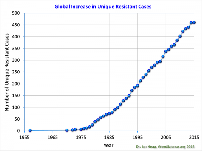
Similar to other pests, weeds evolve resistance when exposed to the same strong selective force, such as an application of the same herbicide over consecutive years. When the same herbicide is applied numerous times to a field, susceptible weeds are killed, leaving resistant individuals to reproduce and dominate the population, as illustrated in figure 8.2.9 below.
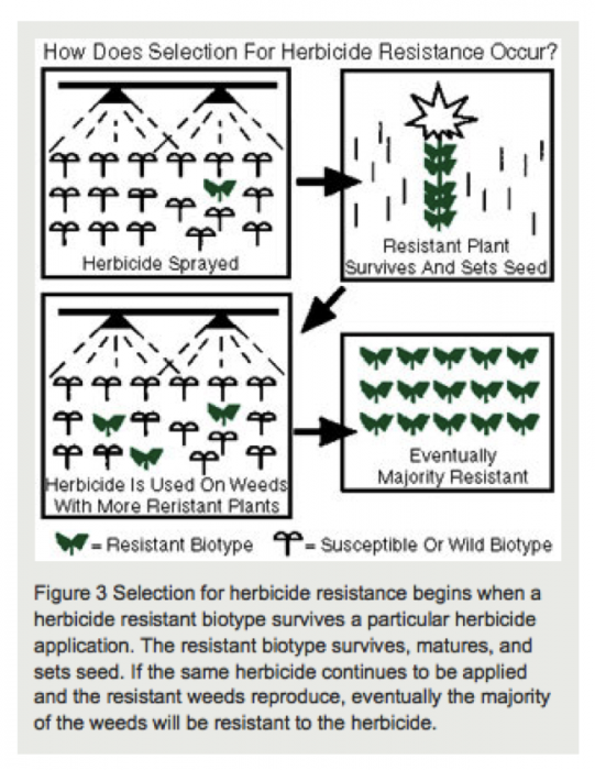
Integrated Weed Management
Integrated weed management (IWM) is an IPM approach for weeds that can provide long-term weed control of weeds by integrating multiple control strategies. Some weed scientists have described IWM as utilizing “many little hammers” as opposed to continuously employing one “big hammer” such as an herbicide (Liebman & Gallandt, 1997). Weed control tactics fall into the IPM control categories that you learned about for insect control in Module 8.1. Examples of weed control practices include the following:
-
Cultural control practices are management practices humans can employ to prevent weed establishment and maintain vigorous crop growth. Examples include: crop rotation with crops of different life cycles and seeding densities, planting certified seed that is managed to have minimal weed contamination, planting adapted crop varieties, adjusting row spacing, population density, and timing for a competitive crop and successful crop establishment, maintaining soil health and fertility, and using practices that prevent weed establishment such as cover crops and mulching.
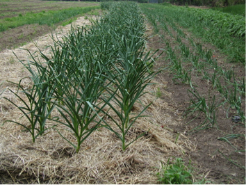 Figure 8.2.10: Straw mulch to suppress weeds in garlic.Credit: Heather Karsten
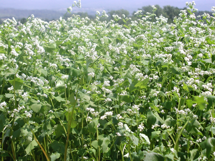 Figure 8.2.11: Buckwheat (Fagopyrum esculentum L. ) cover crop planted mid-season to smother weeds, produce organic matter and provide habitat for beneficial insects.Credit: Anna Santini
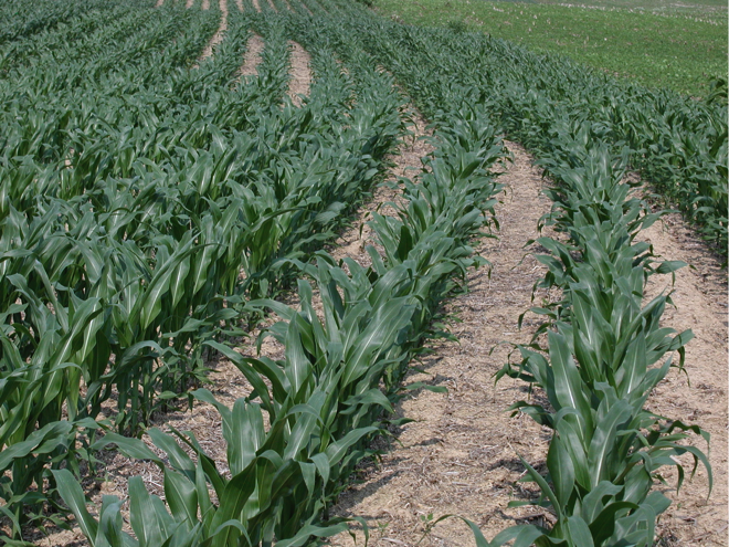
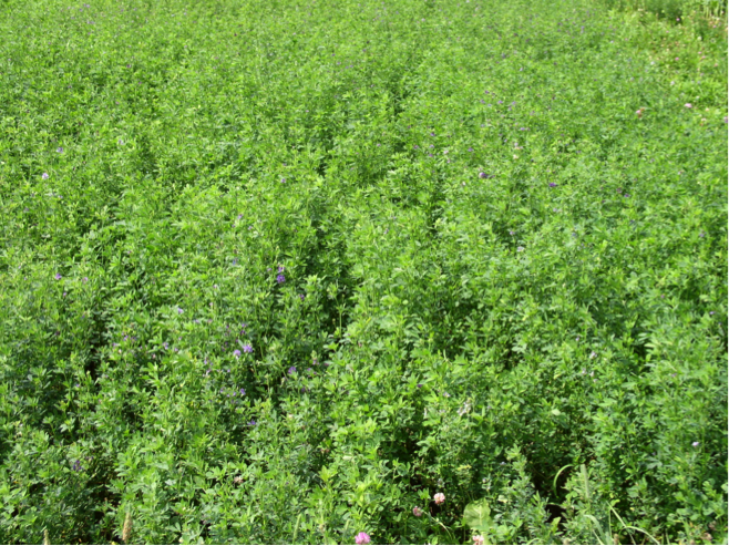
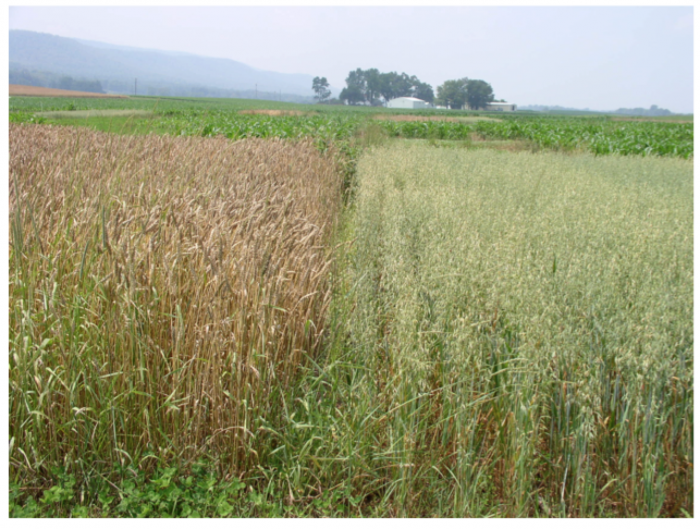 Figure 8.2.12: Crop rotation of summer annual row crops such as corn (first photo) with densely seeded perennial alfalfa (second photo), and/or densely planted winter annual wheat and spring oats (third photo, wheat is on the right, oats are on the left).Credit: Heather Karsten
 - Mechanical or physical weed control includes practices such as plowing, cultivation, hoeing, targeted hand-weeding, and flaming.
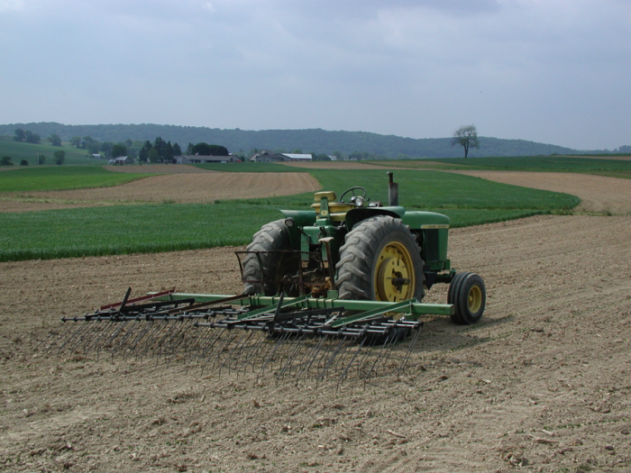 Figure 8.2.13: This flex tine cultivator is used to control weeds when they are very small.Credit: Heather Karsten
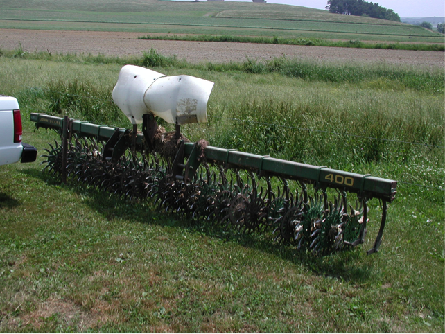 Figure 8.2.14: Rotary harrow for weed cultivation.Credit: Heather Karsten
 - Biological control: conserving or introducing herbivorous insects, grazing or browsing animals, or plant pathogens to reduce weed populations. Biological control of weeds is typically used on extensive rangeland where other more labor intensive or expensive methods are not cost effective.
- Chemical control: the application of herbicides, or the use of herbicide-resistant crops with herbicide applications to control weeds
- Genetic resistance: selecting crop varieties that are well adapted to an environment and competitive with weeds. Herbicide-resistant crops may also be considered a form of genetic resistance.
Transgenic Crops for Pest Control
Transgenic Crops for Pest Control
Transgenic crops or animals are often referred to as GMO’s or genetically modified organisms. This is misleading because all cultivated crop plants and livestock have been genetically modified through centuries of human selection and traditional breeding. A more accurate name for the genetically engineered organisms that are referred to as GMOs, is transgenic organisms. Transgenic crops or livestock contain genetic material that was transferred from a different species through biotechnology techniques or genetic engineering.
In the 1980s, agricultural input companies began developing and using transgenic techniques to develop new crop varieties. The first traits that were inserted into major crop plants and commercialized on a large scale were genes from two different species of bacteria. The transgenic traits were for insect resistance (Bt) and resistance to the herbicide glyphosate (commercially marketed as Round-up). Since the first commercial release in 1996, these technologies have been widely adopted in the US and other parts of the world (See Figure below).
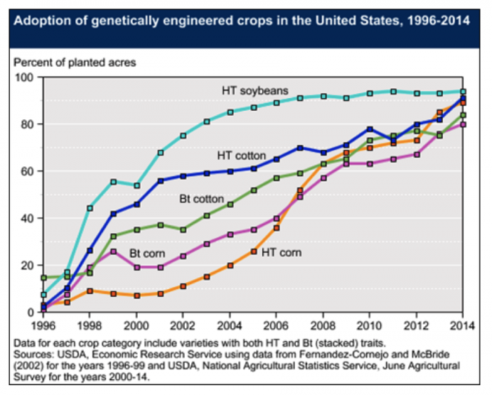
Insect Resistant Bt Crops
Insect Resistant Bt Crops
Bt is an abbreviation for Bacillus thuringiensis a bacteria that produces an enzyme that is toxic to the digestive system of insects in the Beetle; and Moth and Butterfly families. These two insect families include some major crop pests. Scientists have transferred the genes that code for the production of the toxins into crop plants. Because the Bt trait confers insect pest resistance, the adoption of Bt corn and Bt cotton has contributed to a significant reduction of insecticide use in these crops (See Figures 8.2.16- 8.2.18 below).
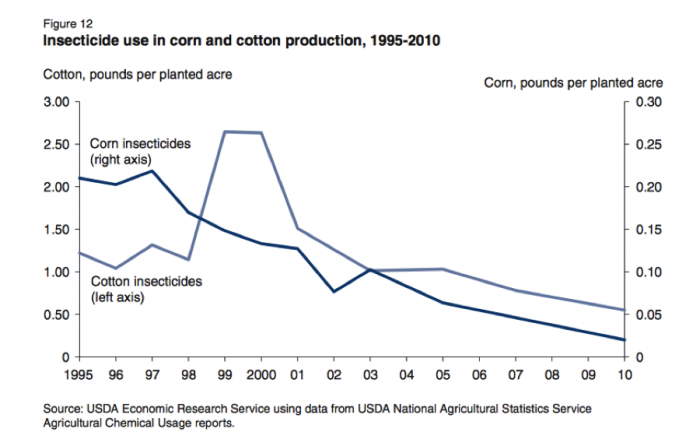
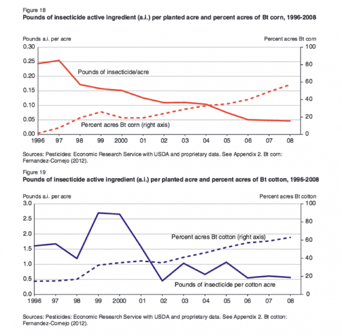
Figure 8.2.18: (Figure 19) Pounds of insecticide active ingredient (a.i.) per planted acre and percent acres of Bt cotton, 1996 - 2008.
Reading
Read this summary of the use and impact of Bt corn, in the following online article “Use and Impact of Bt Maize [15]” by: Richard L. Hellmich (USDA–ARS, Corn Insects and Crop Genetics Research Unit, and Dept of Entomology, Iowa State Univ, IA) & Kristina Allyse Hellmich (Dept. of Biology, Grinnell College, IA). 2012 Nature Education.
Check Your Understanding
Many Bt corn hybrids marketed today contain Bt Cry proteins that are toxic to the corn rootworm and are “stacked” or “pyramids”. To what does this stacked or pyramid in Bt hybrids refer?
Click for the answer.
Name three benefits of Bt corn for farmers.
Click for the answer.
To prevent the evolution of pest resistance to Bt, what practices are most recommended?
Click for the answer.
Prior to the development of Bt crops, spores of the bacteria Bacillus thuringiensis were sometimes used as biological control for insect pests in forestry and agriculture, often on organic farms. Initially, commercial Bt crops were released in the US without any regulations to prevent resistance. But science had shown that pest populations could quickly evolve resistance to Bt, and planting Bt crops on a large scale across the agricultural landscape would create a strong selective force for pests to evolve resistance to Bt. Therefore, in response to public concern about the high risk of pests evolving resistance to Bt, the EPA convened a committee that developed a resistance management plan for Bt crops.
In addition to the crop expressing a high dose of the Bt toxin, to prevent or delay pest resistance to Bt farmers who plant transgenic Bt corn and cotton, are required to plant a refuge, a percentage of the crop field or a field close by that does not express the Bt trait. The refuge area conserves a population of insects that are susceptible to Bt, so that the susceptible insects can reproduce with insects that might have resistance to Bt, sustaining some Bt-susceptible individuals in the population. Depending on the presence of Bt crops in a region, the EPA regulation requires that farmers plant between 5% and 20% of their crop field without the Bt trait. For stacked Bt corn hybrids (with 2 or more Bt traits) farmers must plant the required refuge for each Bt trait that their crop expresses. For more information on refuge requirements, read Insect Resistance Management and Refuge Requirements for Bt Corn [49], from the University of Wisconsin.
Pest Resistance to Transgenic Bt Crops
Despite the refuge requirement in the US, western corn rootworm resistance to Bt corn was reported in multiple Midwestern states (Jakka et al., 2016). The first reported Bt-resistant corn rootworm populations were found in cornfields in Iowa that had been planted to Bt corn consecutively for at least three years, and the authors suggested that the fields likely did not include refuge corn (Gassman et al., 2011). Additional studies also found that the Bt toxin dose was not sufficiently high to delay the evolution of insect resistance and that corn rootworm could evolve resistance to additional Bt toxins in three to seven generations (Gassman, 2016). Further, in 2013 pest resistance to Bt crops was reported in 5 of 13 major pest species in a survey of 77 studies from eight countries across five continents, where resistance management requirements and enforcement varied. Practices that delayed resistance to Bt included the Bt crop expressing a high dose of the Bt toxin and an abundance of refuge crop planting (Tabashnik, et al., 2013). In accordance with integrated pest management principles, entomologists also recommend that other control tactics be utilized to control pests targeted by Bt crops.
In a number of countries (ex. most countries in the European Union), Bt crops and transgenic crops were not approved for commercial production. Concerns about the potential human health and ecological risks of transgenic crops limited acceptance of Bt crops and other transgenic crops. Applying the precautionary principle, some policy-makers and the public require more research and long-term assessment of transgenic traits on human health and ecosystems. An interest in protecting domestic seed markets and companies may also contribute to policy decisions to prohibit the adoption of transgenic seeds produced by multi-national seed companies.
Herbicide Resistant Crops
Herbicide Resistant Crops
Herbicide-resistant (or tolerant) crops, such as glyphosate-resistant crops are transgenic crops that are resistant to the herbicide glyphosate. Glyphosate is a broad-spectrum herbicide that controls a wide range of plants and breaks down relatively quickly in the environment; it was first marketed under the trade name: Round-up. Round-up Ready soybeans were released in the US in 1996, and since then, additional glyphosate-resistant crops (corn, cotton, canola, sugarbeet, and alfalfa) have been developed and widely adopted in the US and other countries (Fernandez-Cornejo J. and S. J. Wechsler, 2015; Benbrook, 2014; Duke and Powles, 2009). See Figure 8.2.15 on the Transgenic Crops for Pest Control page: Adoption of genetically engineered crops.
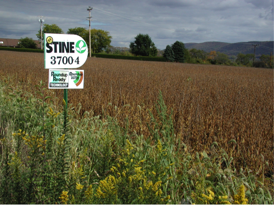
Herbicide-resistant (HR) crops such as glyphosate-resistant crops have facilitated the increased adoption of no-till or direct seeding of some HR crops because tillage is not needed for weed control. Once a crop has emerged, the risk of glyphosate herbicide damage to the HR crop is eliminated, making it easier for farmers to plant crops and control weeds without tillage. However, although Bt crops reduced insecticide use, the glyphosate herbicide must be applied to glyphosate-resistant crops to control weeds. Since they were first introduced in 1996, glyphosate use has increased. See the Figure 8.2.20 from the USGS Pesticide National Synthesis project below.
In addition, in contrast to Bt crops, the EPA did not require farmers to employ a glyphosate resistance management plan or refuge, and the number of weeds that are resistant to glyphosate has increased. Weeds have evolved resistance to glyphosate particularly in cases where farmers consistently applied glyphosate to manage weeds in HR crops and terminated cover crops and/or perennials with glyphosate prior to planting an HR crop. See the Figure 8.2.21 from the International Survey of Herbicide Resistant Weeds illustrating the increase in glyphosate-resistant weeds below.
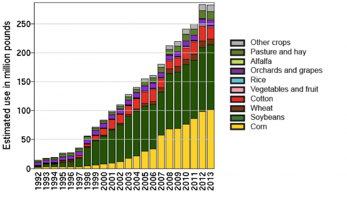
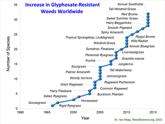
Stacked Herbicide-Resistant Crops
When the number of glyphosate-resistant weeds increased and became difficult to control, the agricultural-input industry developed transgenic herbicide-resistance crops that are resistant to additional herbicides. Dow AgroSciences developed a transgenic trait for resistance to 2,4-D, an herbicide that controls broadleaf weeds (dicot plants) and the company stacked or added the trait to soybean and cotton crops that also have resistance to glyphosate. And Monsanto produced a transgenic trait for resistance to an herbicide called dicamba that they stacked (or added to) soybeans that have glyphosate resistance. Dicamba and 2,4-D herbicides are volatile, and there is a risk that when the herbicides are sprayed, they will drift into neighboring fields and field edges, potentially damaging other crops and other plants. Wild plants in field edges and natural ecosystems often provide habitat for beneficial organisms, such as pollinators, pest predators, and wildlife. In 2017, Monsanto's crops with stacked dicamba and glyphosate resistance were available for use in some midwestern and southern states, where glyphosate-resistant weeds were particularly problematic. In 2017, there were so many reports and complaints from farmers about crop damage due to dicamba drift, that the states of Arkansas and Missouri banned dicamba spraying for some of the growing season. The EPA also investigated the complaints, and in autumn 2017, the EPA announced that the companies had agreed to new steps to reduce the risk dicamba drift with dicamba-resistant crops. For more information, see the EPA Registration of Dicamba for Used on Genetically Engineered Crops. [52]
We will explore concerns about the stacked, herbicide-resistant technologies and tactics to manage glyphosate-resistant weeds more in the Summative Assessment.
Plant Pathogens
Plant Pathogens
Pathogens include fungi, bacteria, nematodes, and viruses, all biological organisms that can cause disease symptoms and significantly reduce the productivity, quality, and even cause the death of plants. Pathogens can also infect agricultural animals, but for this module, we will focus on plant pathogens. Read the following brief overview of plant pathogens, Plant Disease: Pathogens and Cycles [53].
Pathogens can be introduced and spread to host plants in many ways. Bacteria and fungal spores can be transferred by wind, in rain, and from the soil via rain splashing onto plant tissues. Insects can vector or infect a plant with a pathogen when they feed on an infected host plant, and then move and feed on an uninfected plant. Pathogens can also spread through infected seeds, transplants, or contaminated equipment, irrigation water, and humans.
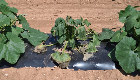
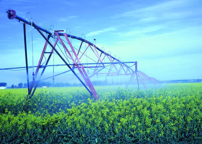
Plant Disease Triangle: Plant pathologists have identified three factors that are needed for a plant disease to develop:
i. a susceptible host Some pathogens have a narrow host plant range, meaning they can infect just a few host species. For instance, the primary host crops of Late blight (Phytophthora infestans) are tomato and potato. For more information see Tomato-Potato Late Blight in the Home Garden [55]. By contrast, pathogens with a wide host plant range can infect many different host species. There are almost 200 plant species that can be infected by Bacterial wilt (Ralstonia solanacearum). For more information, see Bacterial Wilt - Ralstonia solanacearum [56].
ii. a disease-causing organism (pathogen). Plant pathogens include fungi, bacteria, viruses, and nematodes. For examples, again, see the reading: Introduction to Plant Diseases [18], A. D. Timmerman, K.A. Korus. 2014. University of Nebraska-Lincoln. Extension. EC 1273.
iii. a favorable environment for the pathogen. Pathogens usually require specific humidity and temperature conditions for pathogen infection and disease symptoms to manifest. For instance, Late Blight disease symptoms are most likely to occur when the weather is cool and wet.
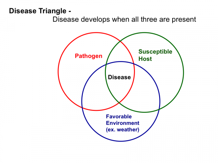
Disease Diagnosis
The three disease triangle factors are important for diagnosing the cause of disease symptoms. Pathologists consider the weather, environmental conditions and the host species to diagnosis what pathogen is causing disease symptoms. Pathologists also consider other factors that could favor and help diagnose a disease, such as i. the field history, particularly what crops and pathogens were present in the past, ii. current crop management practices, iii. when disease symptoms were visible, and on what other species. To assist farmers and others with disease diagnosis, many land-grant universities in the US have crop and animal diagnostic disease clinics where one can submit diseased tissue samples with detailed information that can aid in the diagnosis, such as the host species, environmental conditions, the site history, and management.
Pathogen Management
Although disease control practices could be categorized into the pest control approaches that were discussed earlier for managing insects and weeds (genetic, cultural, chemical, etc.), plant pathologists typically describe pathogen control tactics with more specific language. For instance, Exclusion tactics involve rejecting infected transplants from being introduced to a farm.
Prevention or Avoidance of pathogen introduction and spread tactics include:
- crop rotation, particularly for pathogens with narrow host ranges
- sanitizing equipment for planting, trellising, pruning, and harvesting
- managing for healthy vigorous crops with optimal soil and water nutrient management
- managing to avoid environmental conditions that promote pathogens, such as avoiding very humid conditions due to over-watering, or promoting drying of plant surfaces with wide row spacing to facilitate air flow, or using drip-tape irrigation that waters plants at or below the soil surface versus over the canopy
- using physical barriers such as row covers, mulch to reduce water splashing; and high tunnel/hoop houses or greenhouses to prevent the introduction of rain and wind-borne pathogens
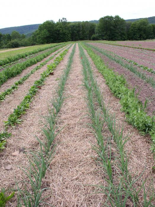
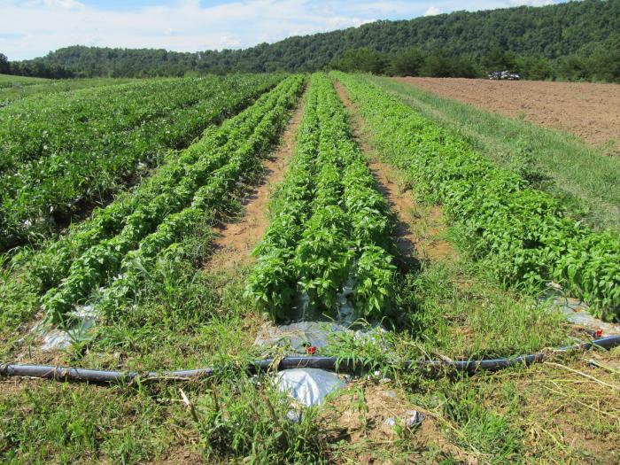
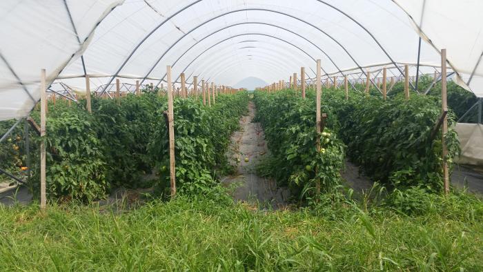
Genetic resistance to pathogens is a very valuable and important pathogen control tool. Many plant breeding programs select for genetic resistance to pathogens. When available, pathogen resistance traits are included in most crop variety descriptions to help growers select appropriate crop varieties for their farm.
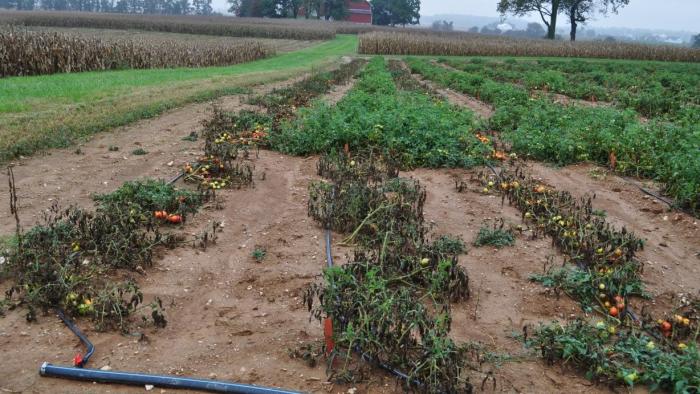
If disease symptoms develop, infected plants may be Eradicated or destroyed. And materials that may have been contaminated with pathogens, such as the soil and planting containers, can be heated to very high temperatures with pasteurization equipment or through solarization. For instance, soil may be solarized by placing black plastic over the crop bed (planting zone) during the warm season to increase the soil temperature and destroy pathogens prior to planting the crop.
Therapy or Fungicides (chemical control) may be applied to infected plants to terminate pathogens. Particularly when plant pathogen symptoms are identified early and favorable weather conditions for the pathogen are projected to continue, fungicides can prevent disease spread and significant economic losses. In some high-value crop systems, the soil may be fumigated prior to planting crops.
Similarly, in agricultural livestock systems, animals with disease symptoms can be treated with antibiotics. And in some livestock production systems, antibiotics and vaccinations are administered to animals to prevent diseases and pathogen infection.
Activate Your Learning
Read Nonchemical Disease Control [57], from Colorado State University Extension and identify some pathogen control tactics that could also qualify as other types of pest control categories that we have explored in this module (such as genetic, cultural, and chemical control).
Click for the answer.
- Cultural control strategies: Prevention and Avoidance through crop rotation and management of the crop environment. Exclusion and Eradication of inoculum through sanitation to the survival of plant pathogens on crop residues and agricultural equipment and managing for healthy vigorous crop growth.
- Genetic: Resistance, Selecting and breeding crop varieties for resistance to plant pathogens is one of the primary means of disease management, particularly in agronomic crops.
- Chemical: Fungicides that are toxic to pathogens
- Physical or mechanical: Protection of crops via barriers such as plant netting or soil mulching. Eradication could also be qualified as a physical control strategy
- Regulatory: Quarantines
Summative Assessment: Herbicide-Resistant Weed Interpretation and Management of Multiple Pest Types
Summative Assessment: Herbicide-Resistant Weed Interpretation and Management of Multiple Pest Types
Note
Please read through the entire assignment before you begin the assignment. Once you have done that, return here to follow the link and review the information.
Explore the International Survey of Herbicide Resistant Weeds [51] to examine the trends of herbicide-resistant weeds and answer the questions below. By going to the "US State Map [58]" to click on different states and "map of different countries [59]" to move your cursor over different counties, compare the number of herbicide-resistant weed species across a range of geographical regions.
You will also use the following information in the proposed scenario:
Dow AgroSciences developed a transgenic trait for resistance to 2,4-D, an herbicide that controls broadleaf weeds (dicot plants), that has been transferred to soybean, corn, and cotton crops. The trait is stacked or added to soybeans that also have resistance to glyphosate, and another herbicide called glufosinate.
Monsanto has produced a transgenic trait for resistance to an herbicide called dicamba, that they are stacking (or adding to) soybeans that have glyphosate resistance. Some formulations of the dicamba herbicide are volatile, and there is a risk that when farmers spray dicamba it will drift into neighboring fields and field edges, potentially damaging other crops and wild plants in field edges and natural ecosystems. These field edges and other plants often provide habitat for beneficial organisms, such as pollinators, pest predators, and wildlife.
Please also read these short NPR articles on dicamba:
With ok from EPA use of controversial weedkiller is expected to double [60]
A wayward weed killer divides farm communities harms wildlife [61]
If you are interested in more information about the use of dicamba and Arkansas' recent restrictions on the herbicide you may read or listen to the following brief (3-minute) story: Arkansas defies Monsanto moves to ban rogue weed killer [62]
Directions
Read the following scenario and in approximately 450-500 words answer the questions below. I suggest you write your response in a separate document and then copy and paste it into Canvas. Once you have posted your own answers, you need to respond to ONE classmate. Your response should be approximately 150 words.
Assume you manage a 200-acre corn and soybean farm in Southern Pennsylvania. You keep up with the latest technological advances in farming and use seeds from either Dow or Monsanto depending on what your seed salesperson recommends. You are proud of your farm and strive to keep your crops free from both weeds and harmful insects that could damage your crop and cut into your profits. Your immediate neighbors on the East side have a large organic vegetable production farm. Based on what you have observed on the above website, the information mentioned above, and from what you have learned through the readings in this module, answer the following questions:
- What are some potential problems you might encounter if you adopt seeds with the new herbicide traits listed above? How do these problems differ between now and in the future?
- What other weed-control strategies could you use to control glyphosate-resistant weeds?
- How might your pest management system affect your neighbors?
- Are there strategies you can use to mitigate potential harm to your neighbors’ fields?
- If you were farming in Thailand or Egypt instead of in Pennsylvania, what might explain differences in the number of herbicide-resistant species you encounter there compared to your farm in the United States?
- If you farmed in Canada, Australia, or Western Europe what might explain the herbicide-resistant species you encounter there?
Consider the following possible questions when responding to a classmate:
- How do their answers differ from yours?
- Are there suggestions you can make to help them improve their IPM practices-for weeds as well as insects?
- Do they have possible solutions you could use on your farm?
- Is there a question you have about why or how they answered the way they did?
Files to Download
Module 8 Summative Assessment Worksheet [63]
Submitting Your Assignment
Submit your response in Module 8 Summative Assessment Discussion in Canvas.
Summary and Final Tasks
Summary
Scientists have identified and continue to study and develop strategies to reduce the impact of pests in agriculture. Pest species that are subject to one or few pest control practices over time inevitably develop resistance to the strong selective force. Multiple biological factors and ecological processes, however, influence host-pest population interactions, providing many opportunities to combine pest control tactics and identify new pest control approaches. Climate change will also pose new pest challenges. Some of these challenges are discussed in the online resource that you read parts of in Modules 4 and 5. We highly encourage you to read this a short summary of some of the research on Climate Change Impacts in the United States [64]. See Section title: Key Message 2: Weeds, Diseases, and Pests.
Reminder - Complete all of the Module 8 tasks!
You have reached the end of Module 8! Double-check the to-do list on the Module 8 Roadmap [65] to make sure you have completed all of the activities listed.
References and Further Reading
Benbrook. C. 2014. Impacts of genetically engineered crops on pesticide use in the U.S. -- the first sixteen years. Environmental Sciences Europe 2012, 24:24. doi:10.1186/2190-4715-24-24
Duke. O. S. and S. B. Powles. 2009. Glyphosate-Resistant Crops and Weeds: Now and in the Future AgBioForum, 12(3&4): 346-357
Gassmann A.J., Petzold-Maxwell J.L., Keweshan R.S., Dunbar M.W. 2011. Field-evolved resistance to Bt maize by western corn rootworm. PLoS One. [66] 2011:6(7):e22629. doi: 10.1371/journal.pone.0022629. E pub 2011 Jul 29.
Gassman, A. J. 2016. Resistance to Bt maize by western corn rootworm: insights from the laboratory and the field. Current Opinion in Insect Science. 15: 111-115. doi.org-10.1016/j.cois.2016.04.001.
Georghiou. G. P. 1986. The Magnitude of the Resistance Problem. Chapt 1. 14-44. In Pesticide Resistance: Strategies for the Management. Eds. Committee on of Pest Populations; Board of Agriculture, National Research Council.
Gunsolus, L. J. Weed Science, Department of Agronomy and Plant Genetics. Herbicide-resistant weeds [45].
International Survey of Herbicide Resistant Weeds [51].
Jakka, S. R. K., R.B. Shrestha, and A. J. Gassmann. 2016. Broad-specture resistance to Bacillus thuringiensis toxins by western corn rootworm (Diabrotica virgifera vergifera). Scientific Reports. 6:27860. doi:10.1038/srep27860.
Liebman, M. and E. R. Gallandt. 1997. Many little hammers: ecological management of crop-weed interactions. Pages 291–343 in L. E. Jack- son, ed. Ecology in Agriculture. San Diego, CA: Academic.
Odum, E. P. 1997. Ecology: A Bridge Between Science and Society. Snauer Associates: Sunderland, MA.
Stern, V. M., Smith, R. F., van den Bosch, K. & Ragen, K. S. 1959. The integration of chemical and biological control of the spotted alfalfa aphid: the integrated control concept. Hilgardia 29:81-101.
Tabashnik B., Brevault, T., Carriere, Y. 2013. Insect resistance to Bt crops: lessons from the first billion acres. Nature Biotechnology 31: 510-521.
Additional Reading:
- FAO UN More About IPM [67]
- Cornell University’s Pesticide Safety Education Program (PSEP) [68] Part of the Pesticide Management Education
- Cullen, E., and R. Proost, D. Volenberg. 2008. Insect Resistance Managment and Refuge Requirements for Bt Corn [49]. University of Wisconsin Extension. Pest and Nutrient Management Program.
Module 9: Food and Climate Change
Module 9: Food and Climate Change
Introduction
We've seen in previous modules how crucial climate is in food production. Temperature and precipitation are critical factors in the growth of crops, choice of crops, and food production capacity of a given region. In this module, we'll first review the mechanism and projected effects of human-induced climate change. We'll also explore the role that agriculture plays in contributing to human-induced climate change. In the second half of this module, you'll explore the varied impacts that climate change may have on agricultural production. The summative assessment for this module will be an important contribution to your capstone project, as you'll be exploring the potential future climate changes in your assigned regions, and begin proposing strategies to improve the resilience of your assigned region.
Goals and Learning Objectives
Goals and Learning Objectives
Goals
- Outline the basic science behind human-induced climate change and the contribution from agriculture.
- Compare various potential impacts of climate change on our global and local food systems.
- Select strategies that enhance the resilience of food systems in the face of a changing climate.
Learning Objectives
After completing this module, students will be able to:
- Identify climate variables that affect agriculture.
- Explain possible climate change impacts on crops.
- Summarize the mechanisms of human-induced climate change.
- Explain the role of food systems in contributing to climate change.
- Discuss how climate change impacts food production and yield.
- Evaluate how farmers adapt to climate change.
- Differentiate impacts of climate change on climate variables in different regions.
Assignments
Module 9 Roadmap
Detailed instructions for completing the Summative Assessment will be provided in each module.
| Action | Assignment | Location |
|---|---|---|
| To Read |
|
|
| To Do |
|
|
Questions?
If you prefer to use email:
If you have any questions, please send them through Canvas e-mail. We will check daily to respond. If your question is one that is relevant to the entire class, we may respond to the entire class rather than individually.
If you prefer to use the discussion forums:
If you have any questions, please post them to the discussion forum in Canvas. We will check that discussion forum daily to respond. While you are there, feel free to post your own responses if you, too, are able to help out a classmate.
Module 9.1: Understanding Global Climate Change and Food Systems
Module 9.1: Understanding Global Climate Change and Food Systems
We hear a lot about global climate change and global warming in the news, especially about the controversy surrounding proposed strategies to reduce carbon emissions, but how well do you understand the science behind why our climate is changing and our planet is warming? In this unit, we'll review the basic science that underpins our understanding of global warming. Agriculture is one of the human activities that contributes carbon dioxide to the atmosphere, so we'll consider those contributions and how they can be reduced. Finally, we'll start to look to the future. What are some of the projections for future temperatures? We need to know what the future projections are so that we can plan to make our food systems more resilient to expected changes.
Introduction
Introduction
Understanding the Science of Climate Change: The Basics
Module 9 focuses on how agriculture contributes to global climate and how climate change will affect global agriculture. In addition, we'll explore agricultural strategies for adapting to a changing climate. But, before we explore the connections between global climate change and food production, we want to make sure that everyone understands some of the basic science underpinning global climate change.
Have you ever thought about the difference between weather and climate? If you don't like the weather right now, what do you do? In many places, you just need to "wait five minutes"! If you don't like the climate where you live, what do you do? Move! Weather is the day-to-day fluctuation in meteorological variables including temperature, precipitation, wind, and relative humidity, whereas climate is the long-term average of those variables. If someone asked you what the climate of your hometown is like, your response might be "hot and dry" or "cold and damp". Often we describe climate by the consistent expected temperature and precipitation pattern for the geographic region. So, when we talk about climate change, we're not talking about the day-to-day weather, which can at times be quite extreme. Instead, we're talking about changes in those long-term temperature and precipitation patterns that are quite predictable. A warming climate means that the average temperature over the long term is increasing, but there can still be cold snowy days, and blizzards even!
The two videos below are excellent introductions to the science of climate change. We'll use these videos as your introduction to the basic science behind our understanding of climate change that we'll build on as we explore the connections between climate change and food production in the rest of this module. Follow instructions from your instructor for this introductory section of Module 9.
Optional Video Climate Change: Lines of Evidence
The National Academies of Sciences Engineering and Medicine have prepared an excellent 20-minute sequence of videos, Climate Change: Lines of Evidence, that explains how scientists have arrived at the state of knowledge about current climate change and its causes. Use the worksheet linked below to summarize the story that the video tells about anthropogenic greenhouse gas emissions and the resulting changes in Earth's climate. The narrator speaks pretty quickly, so you'll want to pause the video and rewind when you need to make sure you understand what he's explaining. It's important to take the time to understand and answer the questions in the worksheet because you'll use this information in a future assignment.
If instructed by your instructor, download detailed questions about the Climate Change: Lines of Evidence videos:
- MSWord docx -Climate Change: Lines of Evidence video questions [76]
- pdf -Climate Change: Lines of Evidence video questions [77]
Video: What is Climate? Climate Change, Lines of Evidence: Chapter 1 (25:59)
Another resource you can use to help answer the questions is the booklet that goes with this video: Climate Change: Evidence, Impacts, Choices [78]. It is 40 pages, so you might not want to print it. Use it as an online reference.
Penn State geology professor, Richard Alley's, 45-minute video uses earth science to tell the story of Earth's climate history and our relationship with fossil fuels. There is no worksheet associated with this video.
Optional Video: Earth: The Operators' Manual (53:42)
RICHARD ALLEY: All across the planet, nations and cities are working to reduce their dependence on fossil fuels and promote sustainable energy options.
ANNISE PARKER: Because it's the smart thing, because it makes business sense, and it's the right thing. NARRATOR: In China, Europe, and Brazil, energy innovations are changing how we live. And in the US, every branch of the military is mobilizing to cut its carbon bootprint.
DAVID TITLEY: We really believe that the climate is changing.
RICHARD ALLEY: In this program, we'll share how we know Earth is warming and why and discover what Earth science tells us about clean, green energy opportunities. I'm Richard Alley. I'm a geologist at Penn State University. But my research has taken me around the planet, from Greenland to Antarctica. I'm fascinated by how our climate has changed dramatically and often, from times with ice everywhere to no ice anywhere on the planet. Records of past climate help us learn how our Earth operates. What has happened can happen again. And I know that sometimes, things change really fast. I'm a registered Republican, play soccer on Saturdays, and go to church on Sundays. I'm a parent and a professor. I worry about jobs for my students and my daughter's future. I've been a proud member of the UN Panel on Climate Change. And I know the risks. And I've worked for an oil company and know how much we all need energy. And the best science shows we'll be better off if we address the twin stories of climate change and energy, and that the sooner we move forward, the better. Our use of fossil fuels for energy is pushing us towards a climate unlike any seen in the history of civilization. But a growing population needs more and more clean energy. But I believe science offers us an operator's manual with answers to both of these huge challenges.
[MUSIC PLAYING] NARRATOR: "Earth-- The Operator's Manual" is made possible by NSF, the National Science Foundation, where discoveries begin.
RICHARD ALLEY: Humans need energy. We always have and always will. But how we use energy is now critical for our survival. It all began with fire. Today, it's mostly fossil fuels. Now we're closing in on 7 billion of us, and the planet's population is headed toward 10 billion. Our cities and our civilization depend on vast amounts of energy. Fossil fuels-- coal, oil, and natural gas-- provide almost 80% of the energy used worldwide. Nuclear is a little less than 5%, hydropower a little under 6%, and the other renewables-- solar, wind, and geothermal-- about 1%, but growing fast. Wood and dung make up the rest. Using energy is helping many of us live better than ever before. Yet well over 1.5 billion are lagging behind, without access to electricity or clean fuels. In recent years, Brazil has brought electricity to 10 million. But in rural Ceara, some still live off the grid-- no electricity, no running water, and no refrigerators to keep food safe. Life's essentials come from their own hard labor. Education is compulsory, but studying is a challenge when evening arrives. The only light is from kerosene lamps. They're smoky, dim, and dangerous. Someday, this mother prays, the electric grid will reach her home.
TRANSLATOR: The first thing I'll do when the electricity arrives in my house will be to say a rosary and give praise to God.
RICHARD ALLEY: More than half of China's 1.3 billion citizens live in the countryside. Many rural residents still use wood or coal for cooking and heating, although most of China is already on the grid. China has used energy to fuel the development that has brought more than 500 million out of poverty. In village homes, there are flat-screen TVs and air conditioners. By 2030, it's projected that 350 million Chinese-- more than the population of the entire United States-- will move from the countryside to cities, a trend that's echoed worldwide. Development in Asia, Africa, and South America will mean 3 billion people will start using more and more energy as they escape from poverty. Suppose we make the familiar, if old-fashioned, 100-watt light bulb our unit for comparing energy use. If you're off the grid, your share of your nation's energy will be just a few hundred watts, a few light bulbs. South Americans average about 13 bulbs. For fast-developing China, it's more like 22 bulbs. Europe and Russia, 5,000 watts, 50 bulbs, and North Americans, over 10,000 watts, more than 100 bulbs. Now let's replace those light bulbs with the actual numbers. Population is shown across the bottom and energy use displayed vertically-- off the grid to the left, North America to the right. If everyone everywhere started using energy at the rate North Americans do, the world's energy consumption would more than quadruple. And using fossil fuels, that's clearly unsustainable. No doubt about it-- coal, gas, and oil have brought huge benefits. But we're burning through them approximately a million times faster than nature saved them for us, and they will run out. What's even worse-- the carbon dioxide from our energy system threatens to change the planet in ways that will make our lives much harder. So why are fossil fuels such a powerful, but ultimately problematic, source of energy? Conditions on the waterways of today's Louisiana help us understand how fossil fuels are made and why they're ultimately unsustainable. Oil, coal, and natural gas are made from things-- mostly plants-- that lived and died long ago. It's taken hundreds and millions of years for nature to create enough of the special conditions that saved the carbon and energy and plants to form the fossil fuels that we use. Here's how it works. Plants, like these tiny diatoms encased in silica shells, grow in the upper layers of lakes and oceans, using the sun's energy to turn carbon dioxide and water into more plants. When they die, if they're buried where there's little oxygen to break them down, their chemical bonds retain the energy that began as sunlight. If enough carbon-rich matter is buried deeply enough for long enough, the Earth's heat and pressure turn it into fossil fuel, concentrating the energy that once fed the growing plants. Vary what goes into Earth's pressure cooker and the temperature, and you end up with the different kinds of fossil fuel. Woody plants make coal. Slimy plants, algae, will give you oil, and both of them give rise to natural gas. The fossil fuels formed over a few hundred million years, and we're burning them over a few hundred years. And if we keep doing that, sooner or later, they must run out. But there's a bigger problem with fossil fuels. As we've seen, they're made of carbon, primarily. And when you burn them, you add oxygen, and that makes CO2 that goes in the air. We're reversing the process by which they formed. And if we keep doing this, it must change the composition of Earth's atmosphere. What CO2 does was confirmed by basic research that had absolutely nothing to do with climate change.
REPORTER: A continuance of the Upper Air Program will provide scientific data concerning the physics of the upper atmosphere.
RICHARD ALLEY: World War II was over, but the Cold War had begun. The US Air Force needed to understand the atmosphere for communications and to design heat-seeking missiles. At certain wavelengths, carbon dioxide and water vapor block radiation, so the new missiles couldn't see very far if they used a wavelength that CO2 absorbs. Research at the Air Force Geophysics Laboratory in Hanscom, Massachusetts produced an immense database with careful measurements of atmospheric gases. Further research by others applied and extended those discoveries, clearly showing the heat-trapping influence of CO2. The Air Force hadn't set out to study global warming. They just wanted their missiles to work. But physics is physics. The atmosphere doesn't care if you're studying it for warring or warming. Adding CO2 turns up the planet's thermostat. It works the other way as well. Remove CO2, and things cool down. These are the Southern Alps of New Zealand, and their climate history shows that the physicists really got it right. These deep, thick piles of frozen water are glaciers-- slow-moving rivers of ice sitting on land. But once, when temperatures were warmer, they were liquid water stored in the sea. We're going to follow this one, the Franz Josef, from summit to ocean to see the real world impact of changing levels of CO2. It's beautiful up here on the highest snow field, but dangers lurk beneath the surface. I've spent a lot of time on the ice. It's standard practice up here to travel in pairs, roped up for safety. The glacier is fed by something like six meters of water a year-- maybe 20 meters, 60 feet of snowfall, so really seriously high snowfall. The snow and ice spread under their own weight, and it's headed downhill at something like a kilometer a year. When ice is speeding up a lot as it flows towards the coast, it can crack and open great crevasses that give you a view into the guts of the glacier. Man, this is a big one. 10, 20, 30, meters more, 100 feet or more heading down in here. And we can see a whole lot of the structure of the glacier right here.
MAN: So what we're going to do is just sit on the edge and then walk backwards, and then I'll lower you.
RICHARD ALLEY: Tell me when. OK. Roll her around, and down we go. Snowfall arrives in layers, each storm putting one down. Summer sun heats the snow and makes it look a little bit different than the winter snow. And so you build up a history. In these layers, there's indications of climate-- how much it snowed, what the temperature was. And all of this is being buried by more snow. And the weight of that snow squeezes what's beneath it and turns it to ice. And in doing that, it can trap bubbles. And in those bubbles are samples of old air-- a record of the composition of the Earth's atmosphere, including how much CO2 was in it, a record of the temperature on the ice sheets and how much it snowed. As we'll see, we can open those icy bottles of ancient air and study the history of Earth's atmosphere. This landscape also tells the story of the Ice Ages and the forces that have shaped Earth's climate. Over the last millions of years, the brightness of the sun doesn't seem to have changed much. But the Earth's orbit, and the tilt of its axis, have shifted in regular patterns over tens and hundreds of thousands of years. The orbit changes shape, varying how close and far the Earth gets as it orbits the sun each year. Over 41,000 years, the tilt of Earth's axis gets larger and smaller, shifting some of the sunshine from the Equator to the poles and back. And our planet has a slight wobble, like a child's top, altering which hemisphere is most directly pointed towards the sun when Earth is closest to it. Over tens of thousands of years, these natural variations shift sunlight around on the planet, and that influences climate. More than 20,000 years ago, decreasing amounts of sunshine in the Arctic allowed great ice sheets to grow across North America and Eurasia, reaching the modern sites of New York and Chicago. Sea level fell as water was locked up on land. Changing currents let the oceans absorb CO2 from the air. That cooled the Southern Hemisphere and unleashed the immense power of glaciers, such as the Franz Josef, which advanced down this wide valley, filling it with deep, thick ice. Now we're flying over today's coastline, where giant boulders are leftovers from that last ice age. A glacier is a great earth-moving machine. It's a dump truck that carries rocks that fall on top of it. It's a bulldozer that pushes rocks in front of it, and it outlines itself with those rocks, making a deposit that we call a moraine that tells us where the glacier has been. We're 20 kilometers, 12 miles, from the front of the Franz Josef glacier today. But about 20,000 years ago, the ice was depositing these rocks as it flowed past us and out to sea. The rocks we can still see today confirm where the glacier once was. Now, in a computer-generated time lapse condensing thousands of years of Earth's history, we're seeing what happened. Lower CO2, colder temperatures, more snow and ice, and the Franz Josef advanced. 20,000 years ago, 30% of today's land area was covered by great ice sheets which locked up so much water that the global sea level was almost 400 feet lower than today. And then, as Earth's orbit changed, temperatures and CO2 rose, and the glacier melted back. The orbits set the stage. But by themselves, there weren't enough. We need the warming and cooling effects of rising and falling CO2 to explain the changes we know happened. Today, atmospheric CO2 is increasing still more, temperatures are rising, and glaciers and ice sheets are melting. You can see this clearly on the lake formed by the shrinking Tasman Glacier across the range from the Franz Josef. This is what the end of an ice age looks like-- glaciers falling apart, new lakes, new land, icebergs coming off the front of the ice. In the early 1980s, we would have been inside New Zealand's Tasman Glacier right here. Now we're passing icebergs in a new lake from a glacier that has mostly fallen apart and ends over six kilometers, four miles away. One glacier doesn't tell us what the world is doing. But while the Tasman has been retreating, the great majority of glaciers on the planet have gotten smaller. This is the Columbia Glacier in Alaska. It's a type of glacier that makes the effects of warming easy to see. It's been retreating so fast that the Extreme Ice Survey had to reposition their time-lapse cameras to follow its motion. In Iceland, warming air temperatures have made this glacier simply melt away, leaving streams and small lakes behind. Thermometers in the air show warming. Thermometers in the air far from cities show warming. Put your thermometer in the ground, in the ocean, look down from satellites-- they show warming. The evidence is clear. The Earth's climate is warming. This frozen library, the National Ice Core Lab in Denver, Colorado, has ice from all over, kept at minus 35 degrees. The oldest core here goes back some 400,000 years. Here, really ancient ice from Greenland in the north and Antarctica in the south reveals Earth's climate history. Let's see what cores like this can tell us. First are those layers I mentioned in the New Zealand snow. They've turned to ice, and we can count them-- summer, winter, summer, winter. Like tree rings, we can date the core. Other cores tell other stories. Look at this. It's the ash of an Icelandic volcano that blew up to Greenland 50,000 years ago. Cores hold other, and even more important, secrets. Look at these bubbles. They formed as the snow turned to ice and trapped old air that's still in there. Scientists now are working with cores from Antarctica that go back even further. They tell us, with a very high degree of accuracy, how much carbon dioxide was in the air that far back. Researchers break chunks of ice in vacuum chambers and carefully analyze the gases that come off. They're able to measure, very precisely, levels of carbon dioxide in that ancient air. Looking at the cores, we see a pattern that repeats-- 280 parts per million of CO2, then 180, 280, 180, 280. By analyzing the chemistry of the oxygen atoms in the ice, you can also see the pattern of rising and falling temperature over time-- colder during the ice ages, warmer during the interglacial periods. Now put the two lines together, and you can see how closely temperature and carbon dioxide track each other. They're not exactly alike. At times, the orbits caused a little temperature change before the feedback effects of CO2 joined in. But just as we saw in New Zealand, we can't explain the large size of the changes in temperature without the effects of CO2. This is the signature of natural variation, the cycle of the ice ages driven by changes in Earth's orbit with no human involvement. But here's where we are today. In just 250 years since the Industrial Revolution, we've blown past 380 with no sign of slowing down. It's a level not seen in more than 400,000 years, 40 times longer than the oldest human civilization. So physics and chemistry tell us that adding carbon dioxide to the atmosphere warms things up, and Earth's climate history shows us there will be impacts, from melting ice sheets to rising sea level. But how do we know, with equal certainty, that it's not just more natural variation, that humans are the source of the increasing CO2? When we look at a landscape like this one, we know immediately that volcanoes put out all sorts of interesting things, and that includes CO2. So how do we know that the rise of CO2 in the atmosphere that we see comes from our burning of fossil fuels and not from something that the volcanoes have done? Well, the first step in the problem is just bookkeeping. We measure how much CO2 comes out of the volcanoes. We measure how much CO2 comes out of our smokestacks and tailpipes. The natural source is small. Humans are putting out 50 to 100 times more CO2 than the natural volcanic source. We can then ask the air whether our bookkeeping is right, and the air says that it is. Volcanoes make CO2 by melting rocks to release the CO2. They don't burn, and they don't use oxygen. But burning fossil fuels does use oxygen when it makes CO2. We see that the rise in CO2 goes with the fall of oxygen, which says that the rising CO2 comes from burning something. We can then ask the carbon in the rising CO2 where it came from. Carbon comes in three flavors-- the lightweight, carbon-12, which is especially common in plants, the medium weight, carbon-13, which is a little more common in the gases coming out of volcanoes, and the heavyweight, carbon-14. It's radioactive and decays almost entirely after about 50,000 years, which is why you won't find it in very old things, like dinosaur bones or fossil fuels. We see a rise in carbon-12 which comes from plants. We don't see a rise of carbon-13, so the CO2 isn't coming from the volcanoes. And we don't see a rise in carbon-14, so the CO2 can't be coming from recently living plants. And so the atmosphere says that the rising CO2 comes from burning of plants that have been dead a long time. That is fossil fuels. The CO2 is coming from our fossil fuels. It's us. So physics and chemistry show us carbon dioxide is at levels never seen in human history. And the evidence says it's all of us burning fossil fuels that's driving the increase. But what about climate change and global warming? Are they for real? Here's what those who have looked at all the data say about the future.
MAN: Climate change, energy security, and economic stability are inextricably linked. Climate change will contribute to food and water scarcity, will increase the spread of disease, and may spur or exacerbate mass migration.
RICHARD ALLEY: Who do you suppose said that? Not a pundit, not a politician. The Pentagon. These war games at Fort Irwin, California provide realistic training to keep our soldiers safe. The purpose of the Pentagon's Quadrennial Defense Review, the QDR, is to keep the nation safe. The review covers military strategies for an uncertain world. The Pentagon has to think long-term and be ready for all contingencies. The 2010 QDR was the first time that those contingencies included climate change. Rear Admiral David Titley is oceanographer of the Navy and contributed to the Defense Review.
DAVID TITLEY: Well, I think the QDR really talks about climate change in terms that really isn't for debate. And you take a look at the global temperatures. You take a look at sea level rise. You take a look at what the glaciers are doing-- not just one or two glaciers, but really glaciers worldwide. And you add all of those up together, and that's one of the reasons we really believe that the climate is changing. So the observations tell us that. Physics tells us this as well.
RICHARD ALLEY: What climate change means for key global hotspots is less clear.
DAVID TITLEY: We understand the Earth is getting warmer. We understand the oceans are getting warmer. What we do not understand is exactly how that will affect things like strong storms, rainfall rates, rainfall distribution. So yes, climate change is a certainty, but what is it going to be like in specific regions of the world, and when?
RICHARD ALLEY: One area of particular concern to the Navy is sea level rise.
DAVID TITLEY: Sea level rise is going to be a long-term and very, very significant issue for the 21st century.
RICHARD ALLEY: The QDR included an infrastructure vulnerability assessment that found that 153 Naval installations are at significant risk from climatic stresses. From Pearl Harbor, Hawaii to Norfolk, Virginia, the bases and their nearby communities will have to adapt.
DAVID TITLEY: Even with one to two meters of sea level rise, which is very, very substantial, we have time. This is not a crisis, but it is certainly going to be a strategic challenge.
RICHARD ALLEY: Globally, climate change is expected to mean more fires, floods, and famine. Nations may be destabilized. For the Pentagon, climate change is a threat multiplier. But with sound climate science, Titley believes forewarned is forearmed.
DAVID TITLEY: The good thing is the science is advanced enough in oceanography, glaciology, meteorology that we have some skill at some frames of predicting this. And if we choose to use those projections, we can, in fact, by our behavior, alter the future in our favor. RICHARD ALLEY: Titley and the Pentagon think the facts are in.
DAVID TITLEY: Climate change is happening, and there is very, very strong evidence that a large part of this is, in fact, man-made.
RICHARD ALLEY: The military is America's single largest user of energy, and it recognizes that its use of fossil fuels has to change. The Pentagon uses 300,000 barrels of oil each day. That's more than 12 million gallons. An armored Humvee gets four miles to the gallon. At full speed, an Abrams battle tank uses four gallons to the mile. And it can cost as much as $400 a gallon to get gas to some remote bases in Afghanistan. Fort Irwin is a test bed to see if the Army can operate just as effectively while using less fossil fuel and more renewables. And it's not just Fort Irwin in the Army. At Camp Pendleton, Marines were trained on an energy-saving experimental forward operating base that deployed with them to Afghanistan.
ROBERT HEDELUND: Before any equipment goes into theater, we want Marines to get trained on it. So what are some of the things that we can take hold of right away and make sure that we can make a difference for the warfighter down range? RICHARD ALLEY: They test out different kinds of portable solar power units. They also practice how to purify stagnant water and make it drinkable. The Army and Marines both want to minimize the number of convoys trucking in fuel and water. A report for the Army found that in five years, more than 3,000 service members had been killed or wounded in supply convoys.
ROBERT HEDELUND: And if you've got Marines guarding that convoy, and God forbid, it get hit by an IED, then what are the wounded, what are the deaths involved in that? And are we really utilizing those Marines and that capability the way we should?
RICHARD ALLEY: Generators used to keep accommodations livable and computers running are also major gas guzzlers.
ADORJAN FERENCZY: Right now, what we're doing is putting up a power shade. It has flexible solar panels on the top and gives us enough power to run small electronics, such as lighting systems and laptop computers. It also provides shade over the tent structure. Experimenting with this equipment in Africa proved that it could reduce the internal temperature of the tent seven to 10 degrees.
RICHARD ALLEY: All the LED lights in the entire tent use just 91 watts, less than one single old-fashioned incandescent bulb.
ADORJAN FERENCZY: It's a no-brainer when it comes to efficiency.
RICHARD ALLEY: Light-emitting diodes don't weigh much, but they're still rugged enough to survive a typical Marine's gentle touch.
ZACH LYMAN: When we put something into a military application and they beat it up, it's ruggedized. It's ready for the worst that the world can take. And so one thing that people say is if the military has used this thing and they trust it, then maybe it's OK for my backyard.
RICHARD ALLEY: Renewable energy will also play an important role at sea and in the air. The Navy's Makin Island is an amphibious assault ship with jump jets, helicopters, and landing craft. It's the first vessel to have both gas turbines and a hybrid electric drive, which it can use for 75% of its time at sea. This Prius of the ocean cut fuel costs by $2 million on its maiden voyage. By 2016, the Navy plans to have what it calls a Great Green Fleet, a complete carrier group running on renewable fuels with nuclear ships, hybrid electric surface vessels, and aircraft flying only biofuels. By 2020, the goal is to cut usage of fossil fuels by 50%. Once deployed in Afghanistan, the XFOB cut down on gas used in generators by over 80%. In the past, the Pentagon's innovations in computers, GPS, and radar have spun off into civilian life. In the future, the military's use of renewable energy can reduce dependence on foreign oil, increase operational security, and save lives and money.
JIM CHEVALLIER: A lot of the times, it is a culture change more than anything else. And the Department of Defense, over the years, has proved, time and time again, that they can lead the way in that culture change.
RICHARD ALLEY: If the US military is the largest user of energy in America, China is now the largest consumer on the planet. At 1.3 billion, China has a population about four times larger than the US, so average per-person use in CO2 emissions remain about 1/4 those of Americans. But like the US Military, China is moving ahead at full speed on multiple different sustainable energy options. And it pretty much has to. Cities are congested. The air is polluted. Continued rapid growth using old technologies seems unsustainable. This meeting in Beijing brought together mayors from all over China, executives from state-owned enterprises, and international representatives. The organizer was a US-Chinese NGO headed by Peggy Liu.
PEGGY LIU: Over 20 years, we're going to have 350 million people moving into cities in China. And we're going to be building 50,000 new skyscrapers, the equivalent of 10 Manhattans, 170 new mass transit systems. It's just incredible, incredible scale.
RICHARD ALLEY: This massive, rapid growth comes with a high environmental cost.
MARTIN SCHOENBAUER: They recognize that they're spending as much as 6% of their gross domestic product on environmental issues.
RICHARD ALLEY: In 2009, China committed $35 billion, almost twice as much as the US, TO energy research and incentives for wind, solar, and other clean energy technologies. It's attracted an American company to set up the world's most advanced solar power research plant. China now makes more solar panels than any other nation. But it's also promoting low-tech, low-cost solutions. Solar water heaters are seen on modest village homes. Some cities have them on almost every roof.
PEGGY LIU: China is throwing spaghetti on the wall right now in terms of over 27 different cities doing LED street lighting, or over 20, 30 different cities doing electric vehicles.
RICHARD ALLEY: But visit any city, and you can see that the coal used to generate more than 70% of China's electricity has serious consequences with visible pollution and adverse health effects. China uses more coal than any other nation on Earth, but it's also trying to find ways to burn coal more cleanly.
PEGGY LIU: In three years, 2006 to 2009, while China was building one new coal-fired power plant a week, it also shut down inefficient coal plants. So it's out with the old and in with the new. And they're really trying hard to invent new models.
RICHARD ALLEY: This pilot plant, designed for carbon capture and sequestration, was rushed to completion in time for Shanghai's 2010 World Expo. It absorbs and sells carbon dioxide and will soon scale up to capture 3 million tons a year that could be pumped back into the ground, keeping it out of the air.
MARTIN SCHOENBAUER: Here in China, they are bringing many plants online in a much shorter time span it takes us in the US. PEGGY LIU: China is right now the factory of the world. What we'd like to do is turn it into the clean tech laboratory of the world. RICHARD ALLEY: If nations choose to pay the price, burning coal with carbon capture can offer the world a temporary bridge until renewables come to scale. PEGGY LIU: China is going to come up with the clean energy solutions that are cost-effective and can be deployed at large scale-- in other words, solutions that everybody around the world wants.
RICHARD ALLEY: Can low-carbon solutions really give us enough energy to power the planet and a growing population? Let's put some numbers on how much energy we can get from non-fossil fuel renewables. Today, all humans everywhere on Earth use about 15.7 terawatts of energy. That's a big number. In watts, that's 157 followed by 11 0's, or 157 billion of those 100-watt light bulbs we used as a reference. To show what's possible, let's see if we can get to 15.7 terawatts using only renewable energy. I'm here in the Algodones Dunes near Yuma, Arizona. The Guinness Book of Records says it's the sunniest place in the world. There's barely a cloud in the daytime sky for roughly 90% of the year. 0.01%, 1/100 of 1%-- if we could collect that much of the sun's energy reaching the Earth, it would be more than all human use today. Today's technologies have made a start. This was the world's first commercial power station to use a tower to harvest concentrated solar energy. Near Seville, Spain, 624 mirrors stretch over an area of more than 135 acres, beaming back sunlight to a tower nearly 400 feet high. Intense heat produces steam that drives the turbine, which generates electricity. When completed, this one facility will be able to power 200,000 homes, enough to supply the entire nearby city of Seville. Remember our target of 15.7 terawatts? Well, the sun delivers 173,000 terawatts to the top of Earth's atmosphere, 11,000 times current human use. No way we can capture all of that potential energy at Earth's surface. But the deserts of America's Southwest, with today's technology, have enough suitable land to supply 80% of the entire planet's current use. Of course, there's one big problem with solar power-- night. But with more efficient transmission lines, and as part of a balanced renewable energy portfolio that includes storage, the sun's potential is vast. In tropical nations like Brazil, the sun heats water, makes clouds, and unleashes rainfall that feeds some of the planet's largest rivers. Iguazu Falls is a tourist attraction, one of the most spectacular waterfalls on Earth, where you can feel the immense power of falling water. The nearby Itaipu Dam on the border of Brazil in Paraguay produces the most hydroelectric power of any generating station in the world. This one dam supplies most of the electricity used in Sao Paulo, a city of more than 11 million. Sao Paulo is 600 miles away, but Brazil made the decision to build innovative, high-voltage direct current transmission lines to minimize energy loss. The Itaipu to Sao Paulo electrical grid has been in operation since 1984 and shows that renewable energy can go the distance. Dams can't be the answer for every nation. They flood landscapes, disrupt ecosystems, and displace people. But hydropower gives Brazil, a nation larger than the continental United States, 80% of its electricity. And worldwide, hydropower could contribute 12% of human energy use, ready at a moment's notice in case the sun goes behind a cloud. Brazil is also using its unique natural environment in another way. Its tropical climate provides ideal conditions for sugarcane, one of the Earth's most efficient plants in its ability to collect the energy of sunlight. Plantations like this one harvest the cane for the production of sugar and the biofuel called ethanol. The US is actually the number one producer of ethanol in the world, mostly using corn instead of cane. But ethanol made from sugar cane is several times more efficient at replacing fossil fuel than corn-based ethanol. Modern facilities like this one pipe back wet waste to fertilize the fields and burn the dry waste, called the gas, to generate electricity to run the factory. For Brazil, at least, ethanol works. Today, almost all cars sold in Brazil can use flex fuels. Drivers choose gasoline blended with 25% ethanol or pure ethanol, depending on price and how far they plan to drive. Local researchers say that if all the gasoline in the world suddenly disappeared, Brazil is the only nation that could go it alone and keep its cars running. Using food for fuel raises big questions in a hungry world. As of now, sugarcane ethanol hasn't affected food prices much. But there are concerns with corn. So here in the US, government labs like NREL, the National Renewable Energy Lab, have launched programs to see if biofuels can be made from agricultural waste. It does work, and researchers are trying to bring the cost down. So with plants capturing roughly 11 times human energy use, they're a growing opportunity. New Zealand takes advantage of another kind of energy. These are the geysers and hot springs at Rotorua on the North Island. Once, they were used by the native Maori people for cooking and bathing. Now geothermal power plants harvest heat and turn it into as much as 10% of all New Zealand's electricity. Many power projects are partnerships with the Maori, benefiting the local people and avoiding the "not in my backyard" problems that often complicate energy developments. Globally, geothermal energy offers three times our current use. But we can mine geothermal, extracting the energy faster than nature supplies it, cooling the rocks deep beneath us to make power for people. This energy exists even where you don't see geysers and mud pots, so it can be extracted without harming these natural wonders. A study by MIT showed that the accessible hot rocks beneath the United States contain enough energy to run the country for 130,000 years. And like hydroelectric, geothermal can provide peaking power, ready to go at a moment's notice if the sun doesn't shine and the wind doesn't blow. Mining energy from deep, hot rocks is a relatively new technology, but people have been using windmills for centuries, and the wind blows everywhere. Here's where the United States is very lucky. Let's take a trip up the nation's wind corridor, from Texas in the South to the Canadian border. Bright purple indicates the strongest winds. All along this nearly 2,000 miles, there's the potential to turn a free, non-CO2-emitting resource into electricity. But that takes choices and actions by individuals and governments. Here's what's been happening in West Texas. It's a land of ranches and farms and, of course, oil rigs and pump jacks. But in the early '90s, this was one of the most financially depressed areas in the state. Communities like Nolan Divide fell on hard times. Schools closed. People moved away. But since 1999, the new structures towering above the flat fields aren't oil derricks, but wind turbines. The largest number-- more than 1,600-- is in Nolan County. Greg Wortham is Mayor of Sweetwater, the county seat.
GREG WORTHAM: It wasn't a philosophical or political decision. It was ranchers and farmers and truck drivers and welders and railroads. and wind workers.
RICHARD ALLEY: Steve Oatman's family has been ranching the Double Heart for three generations. Steve may have doubts about the causes of climate change, but not about wind energy.
STEVE OATMAN: But it's been a blessing. It helps pay taxes. It helps pay the feed bill. Rosco, 30 May.
GREG WORTHAM: We talk about this being green energy because it pays money. The ranchers and the farmers call it mailbox money. They have to get up, and sweat, and work hard all day long. Things are pretty stressful. And if you can just walk to the mailbox and pick up some money because you've got turbines above the ground, that makes life a lot easier. RICHARD ALLEY: Each windmill can generate between $5,000 and $15,000 per year. So a ranch with an average of 10 to 20 turbines can provide financial stability for people who have always lived with uncertainty.
STEVE OATMAN: I don't just believe in it because I make a living from it. It's something that's going to have to happen for the country.
RICHARD ALLEY: So now, local schools have growing enrollments and funds to pay for programs.
GREG WORTHAM: We had about $500 million in tax based in the whole county in 2000. And by the late part of that decade, in less than 10 years, it went up to $2.5 billion in tax value.
RICHARD ALLEY: By the end of 2009, the capacity of wind turbines in West Texas totaled close to 10,000 megawatts. If Texas were a country, it would rank sixth in the world in wind power. The US Department of Energy estimates that wind could supply 20% of America's electricity by 2030. New offshore wind farms would generate more than 43,000 new jobs. That translates into a $200-billion boost to the US economy. Worldwide, wind could provide almost 80 times current human usage. No form of energy is totally free of environmental concerns or hefty startup costs. Some early wind farms gave little consideration to birds and other flying critters, like migrating bats. But recent reports by Greenpeace and the Audubon Society have found that properly sighted and operated turbines can minimize problems. Mayor Wortham, for one, welcomes wind turbines into his backyard.
GREG WORTHAM: We like them. Some people don't. But we're more than happy to export our energy to those states who want to buy green, but don't want to see green.
STEVE OATMAN: In the long run, I hope we have wind turbines everywhere they can produce energy. We need them. That's what America is going to have to do. That's the next stepping stone to save ourselves.
RICHARD ALLEY: The state of Texas has invested $5 billion to connect West Texas wind to big cities like Dallas and Fort Worth. Farther south is Houston, one of the most energy-hungry cities in the country. Its port is America's largest by foreign tonnage, and its refineries and chemical plants supply a good portion of the nation. But already, perhaps surprisingly, Houston is the largest municipal purchaser of renewable energy in the nation. 30% of the power city government uses comes from wind, with a target of 50%. And its mayor wants to cut energy costs and increase energy efficiency.
ANNISE PARKER: I want to go from the oil and gas capital of the world to the green and renewable energy capital of the world.
RICHARD ALLEY: Supported by federal stimulus dollars, the local utility is ahead of schedule to install smart meters. These will help consumers economize on energy use. The city has already installed 2,500 LED traffic lights using 85% less energy than traditional incandescent bulbs. That translates into savings of $3.6 million per year. City Hall thinks it can also improve air quality by changing the kinds of cars Houstonians drive.
ANNISE PARKER: If
RICHARD ALLEY: The city already operates a fleet of plug-in hybrids. Now it's encouraging the development of an infrastructure to make driving electric vehicles easy and practical. And in Houston's hot and humid environment, it helps to have an increasing number of energy-efficient, LEED-certified buildings. ANNISE PARKER: We're going to do it because it's the smart thing, because it makes business sense, and it's the right thing.
RICHARD ALLEY: Some estimates are that the US could save as much as 23% of projected demand from a more efficient use of energy.
ANNISE PARKER: Well, if you're going to tackle energy efficiency, you might as well do it in a place that is a profligate user of energy. And when you make a difference there, you can make a difference that's significant.
RICHARD ALLEY: Globally, efficiency could cut the demand for energy by 1/3 by 2030. Bottom line-- there are many ways forward, and we can hit that renewable energy target. And if next-generation nuclear is also included, one plan has the possible 2030 energy mix transformed from one relying on fossil fuels to one that looks like this, with renewables-- sun, wind, geothermal, biomass, and hydropower-- totaling 61%, fossil fuels down to 13%, and existing and new nuclear making up the balance. Another plan meets world energy needs with only wind, water, and solar. And in fact, there are many feasible paths to a sustainable energy future. Today's technologies can get us started, and a commitment to research and innovation will bring even more possibilities. We've traveled the world to see some of the sources the planet offers to meet our growing need for clean energy. There's too many options to cover all of them here. And besides, each nation, each state, each person must make their own choices as to what works best for them. But the central idea is clear. If we approach Earth as if we have an operator's manual that tells us how to keep the planet humming along at peak performance, we can do this. We can avoid climate catastrophes, improve energy security, and make millions of good jobs. For "Earth-- The Operator's Manual," I'm Richard Alley.
NARRATOR: "Earth-- The Operator's Manual" is made possible by NSF, the National Science Foundation, where discoveries begin.
[MUSIC PLAYING] For the annotated, illustrated script with links to information on climate change and sustainable energy, web-exclusive videos, educator resources, and much more, visit pbs.org. "Earth-- The Operator's Manual" is available on DVD. The companion book is also available. To order, visit shoppbs.org, or call us at 1-800-PLAY-PBS.
Optional Follow-up Questions to the Videos
If instructed by your instructor, download the following questions that can be applied to either video:
Understanding the Science of Climate Change
Understanding the Science of Climate Change
At this point, you should have either watched one or two of the videos from the introduction, or you're already familiar with how human activities have resulted in the warming of the planet in the last century. Now, we'll explore some of the latest data from the National Aeronautics and Space Administration (NASA), the National Oceanic and Atmospheric Administration (NOAA), and the Intergovernmental Panel on Climate Change (IPCC) to review and to help us better understand the connections between increases in atmospheric carbon dioxide and climate change.
Data on current atmospheric concentrations of carbon dioxide are collected and compiled by NOAA and can be found at NOAA Earth System Research Laboratory [81]. The longest record of carbon dioxide concentration in the atmosphere is from Mauna Loa in Hawaii and was initiated in the 1950s. The resulting curve is often referred to as the “Keeling Curve” (Figure 9.1.1) after the atmospheric scientist who first began collecting CO2 data.
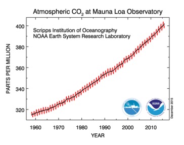
Carbon dioxide is not the only greenhouse gas. Human activities have also increased concentrations of methane and nitrous oxide. The IPCC has compiled data from many sources to summarize the changes in greenhouse gas concentrations for the last 2000 years (Figure 9.1.2), and concentrations of carbon dioxide, methane, and nitrous oxides have all risen dramatically with industrialization. The increases in carbon dioxide concentrations have the greatest impact on global climate, but the increases in the other greenhouse gases play a supporting role.
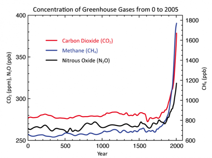
To understand Earth's past climate, scientists use data extracted from air bubbles trapped in ice cores from Greenland and Antarctica to study past carbon dioxide concentrations and temperatures. The longest ice core record is from Vostok, Antarctica and gives us a picture of changes in CO2 concentrations and temperatures for the last 800,000 years (Figure 9.1.3). In November 2015, CO2 concentrations in the atmosphere reached 400.16 ppm, a level not seen in the past 800,000 years on Earth. Also, there is a clear correlation between temperature changes and changes in atmospheric CO2 concentrations.
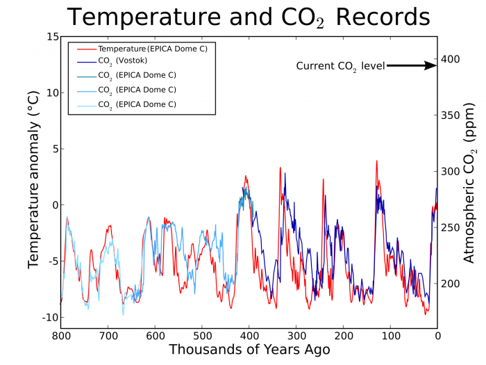
NASA has compiled surface air and ocean temperature data from around the globe and summarized temperature changes into an index (Global Climate Change: Vital Signs of the Planet [85]) that compares annual average temperature with the average temperatures from 1951-1980 (Figure 9.1.4). Global temperatures have been rising for the last 100 years. We'll explore more temperature data and consider the impact of rising temperatures as we continue in this module.
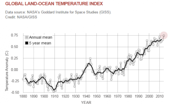
Activate your learning
Question 1 - Short Answer
How does the current concentration of carbon dioxide in the atmosphere compare with atmospheric carbon dioxide concentrations measured in the Vostok ice core (Figure 9.1.3)?
Click for answer.
Current carbon dioxide concentrations (400 ppm in November 2015) are higher than at any time in at least the past 800,000 years.
Question 2 - Short Answer
In the Keeling Curve (Figure 9.1.1), there is a clear upward trend in carbon dioxide concentrations, and there is also a smaller oscillating pattern in the data. Each year, CO2 concentration increase and decrease. What could be causing the annual cycle in carbon dioxide concentrations?
Click for answer.
The annual cycle is a result of the large deciduous forests in the northern hemisphere. Trees take up more CO2 in the summer time when they have green leaves that are taking up CO2 to create new plant material via photosynthesis. In the fall, this process stops. In the winter, when deciduous trees lose their leaves, CO2 levels in the atmosphere increase as photosynthetic rates decline and as CO2 is released as plant material decays. The upward trend, since recording started in the late 1950s, is a result of the burning of fossil fuels and other anthropogenic greenhouse gas emissions.
Question 3 - Short Answer
What is the source of the increasing CO2 concentrations in the atmosphere that is evident in the Keeling Curve (Figure 9.1.1), and that has occurred since about 1850 (Figure 9.1.2)?
Click for answer.
The increase of CO2 concentrations in the atmosphere since 1850 is primarily from the burning of fossil fuels (petroleum, coal and natural gas). Other human activities also contribute, such as deforestation.
Question 4 - Short Answer
Global average temperatures have been increasing since about 1920. Explain the relationship between global temperature increase and increasing levels of CO2 in the atmosphere.
Click for answer.
As carbon dioxide concentrations in the atmosphere increase, more heat energy is trapped in the Earth's lower atmosphere, which results in an increase in temperature. As temperature increases, evaporation rates also increase. Water vapor is a very powerful greenhouse gas, so there is a positive feedback that causes an additional increase in temperature.
Climate is Already Changing
Climate is Already Changing
The impacts of increasing greenhouse gas concentrations are already being felt around the globe, though the degree of change varies with location. The Third National Climate Assessment (NCS), released in 2014 by the US Global Change Research Program (USGCRP), reports that over the last century increasing average temperatures, increasing weather variability, increasing warmer nights and winters, lengthening of the growing season, and an increase in the frequency and intensity of extreme weather events have already been observed. The severity of these impacts varies throughout the US and the world because of regional topography, proximity to the ocean, atmospheric circulation patterns, and many other factors.
Changing Temperature Patterns
The average temperature in the United States has increased in the last century, with each recent decade being warmer than the past, but this warming is not uniform across the United States (Figure 9.1.5). In general, western and northern regions have warmed more than the southeastern US. In the most recent decade, all regions have shown warming. What impact might this warming trend have on our food production and water supply? For example, we know from our study of water for food production that plants evaporate or transpire water and that the rate of evaporation is dependent on temperature. If temperatures go up, we know that plants will transpire more water. The southwestern US is already a water-scarce area, so increasing temperatures will exacerbate that condition.
We'll explore more connections between climate change and food production in the next section of this module. First, let's investigate changes in some other climate variables.
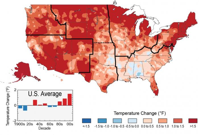
Changing Precipitation Patterns
In addition to changing temperatures, the recent decades have seen changes in precipitation patterns. Nationwide average precipitation has increased (Figure 9.1.6), but the patterns of change are not as clear as those for temperature. Notice in Figure 9.1.6 that the water-scarce Southwest experienced a decline in precipitation in recent decades. Additionally, some of the precipitation increase in the eastern US came in form of extremely heavy precipitation (Figure 9.1.7) and resulted in flooding (Figure 9.1.8). Both of these effects are anticipated results of increased concentrations of heat-trapping greenhouse gases in the lower atmosphere.
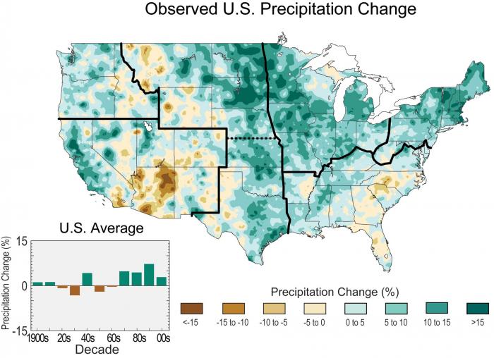
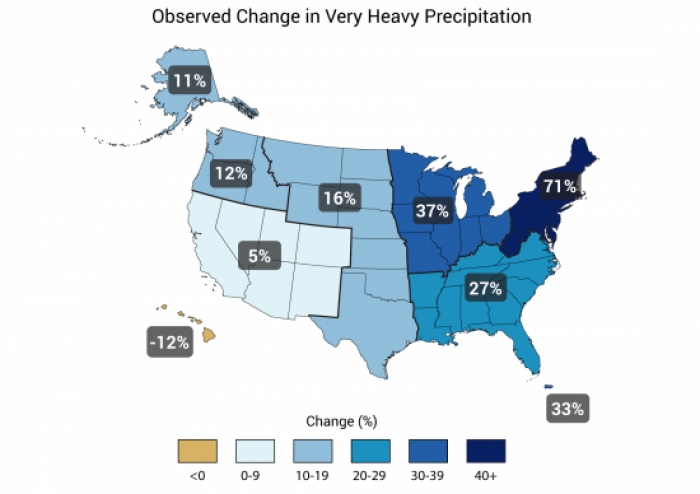
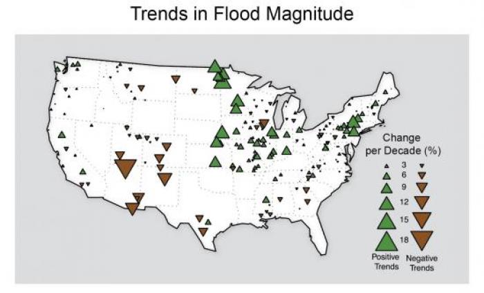
Projected Climate Changes
Projected Climate Changes
So far in module 9, we've studied the basics of the science of climate change and by now you should have a pretty good understanding of the relationship between greenhouse gases and temperature. We've seen how human activities, including our food systems, are contributing carbon dioxide and other greenhouse gases to the atmosphere. And, as greenhouse gas concentrations increase, more heat energy is trapped, so temperatures at the Earth's surface increase.
We've also seen that temperatures are already increasing around the globe and that precipitation patterns are changing, but what does the future hold? How much will temperatures increase? Will precipitation increase or decrease? Those are very good questions! And, the answers aren't perfectly clear. Atmospheric and climate scientists all over the world are working hard to estimate how Earth's climate will change as greenhouse gas concentrations increase. Future predictions are made by running computer models that simulate natural processes and human activities and estimate future conditions. Model results vary from model to model, but they all predict future warming. Also, as we've already seen, the amount of warming varies from place to place.
What are the predictions for future climate?
The models used to predict future climate are very complicated and incorporate a vast number of variables, natural processes, and human activities. Projecting into the future is always a tricky endeavor and is always fraught with uncertainty. However, all of the models predict continued warming in the future. The magnitude of the warming varies from model to model and depending on which carbon emission scenario is used. For example, warming might slow in the future if we manage to curb our burning of fossil fuels, which would result in lower carbon dioxide emissions.
The model results are presented on two websites (National Climate Change View and Global Climate Change Viewer) that allow us to view the future projections for the US and for the globe on easy-to-read maps. In the summative assessment for this module, you'll explore these websites in greater depth to extract data for your capstone assignment. Right now, we'll just look at a few of the maps to get an idea of how the climate is projected to change in the latter part of this century. Exploring these maps develops our spatial thinking skills, which in turn enhances our math skills! And, who doesn't want to be better at math?
Future climate projections are presented as the projected change compared to the latter part of the last century (1950-2005). So for example, if the projected temperature change for 2050-2074 is 4oF, then that means the 2050-2074 average temperature is projected to be 4oF higher than the average temperature from 1950-2005. All of the following maps present projected change in this manner.
First, let's look at temperature. The National Climate Change Viewer (NCCV) (Figures 9.1.9 and 9.1.10) and Global Climate Change Viewer (GCCV) (Figure 9.1.11) both provide maps of projected temperature changes. Notice that the global map gives temperature change in degrees Celsius, and the US map is in Fahrenheit. One notable aspect of all three maps is that temperature is expected to increase everywhere. As you look at these maps, notice where the temperature change is expected to be the greatest. Can you make any generalizations? What is the expected temperature change in the region where you live right now? For example, if we were in New York City, the map in Figure 9.1.9 suggests that the average maximum temperature by 2050-2074 could be 4oF higher than it was in 1950-2005.
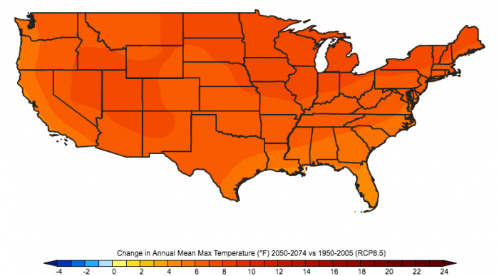
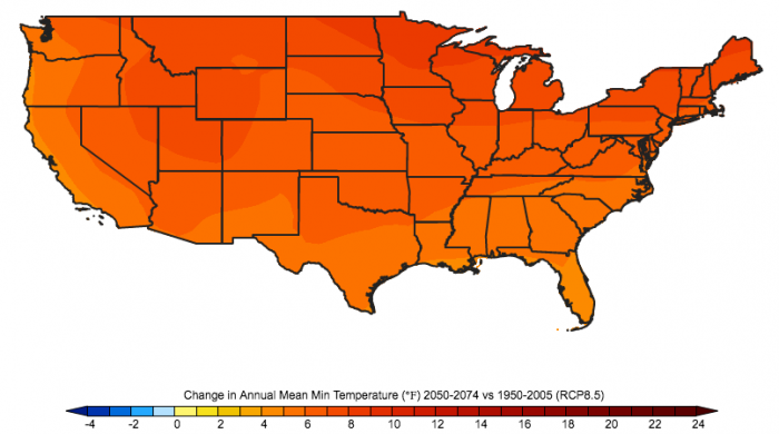
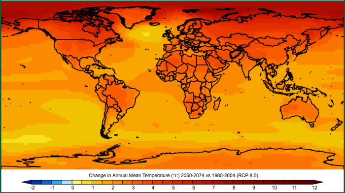
The projected changes in precipitation aren't quite as straightforward or certain as the projected temperature changes. Some regions are expected to receive more precipitation and some regions less. You can see in Figure 9.1.12 the southwestern US, a region that is already water-scarce, is expected to receive less annual precipitation on average. On the global map in Figure 9.1.13, equatorial regions are expected to receive a little more precipitation, and there's a band just north and south of the equator where precipitation is expected to decrease. The certainty in the precipitation predictions is lower than for temperature and the variability within a given year and from year to year in how the precipitation falls is expected to increase.
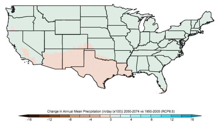
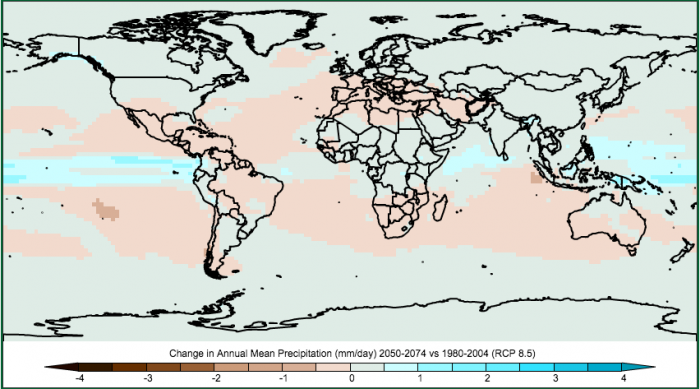
The NCCV also allows you to view projected changes in a few more variables that are not available on the GCCV. Students studying food regions outside of the US will need to work with their instructor to find similar data for their regions.
Precipitation falls on the land surface and flows into streams and rivers, which is called runoff. If precipitation is projected to decrease in the future, it would make sense that runoff would also decrease. Also, as temperatures increase and cause evaporation and transpiration to increase, there is less water available to run off into streams and rivers. The NCCV runoff map (Figure 9.1.14) suggests that runoff will also decrease in many areas of the US. The units for runoff are given in inches of water per month, similar to units for precipitation. In water-scarce regions where the precipitation is low, for example in deserts, often agriculture is irrigation with runoff from upstream regions where the precipitation is higher. Decreases in runoff could have adverse impacts on some regions that rely on runoff for irrigation.
As temperatures increase, there is an expected decrease in annual snowpack. While this is bad news for avid skiers, it's also bad news for regions that rely on water stored in snowpack in the winter that melts and is used for irrigation in the summer months. Figure 9.1.15 illustrates the projected change in annual mean snow in inches. Regions that don't normally get snow are indicated as zero (the deep south and southwest). The Rockies, Sierra Nevadas, Cascades as well as the mountains in the northeast are all expected to see significant decreases in annual snowpack.
The combination of increased temperatures with increased evaporation and transpiration rates will leave soils drier. Soil moisture content is projected to decrease across much of the US (Figure 9.1.16). Soil moisture is measured in units of depth of water (inches) and is the water available to plants. Some of our very important agricultural regions, the Midwest, are expected to see some of the largest declines in soil moisture storage.
The last data set, evaporative deficit, (Figure 9.1.17) gives us an idea of how much water could evaporate compared to how much water is actually available. An increase in evaporative deficit is a symptom of a transition to a hotter and drier climate. Not surprisingly the entire US is projected to see an increase in evaporative deficit, with the highest increases being in the Southwest and Midwest.
In summary, the future projected climate for the US is generally hotter and drier. Precipitation projections are more variable and less certain, but the increase in temperature and resulting increase in evaporation and transpiration will result in less runoff and drier soils in much of the US. The implications for agriculture are significant. We've already seen how water is essential for crop growth and changes in the temperature regime may have some surprising impacts on growing our food. In the next section, we'll explore projected climate changes and the potential impacts on agriculture in more detail. We'll also consider some possible adaptation strategies that can make our food systems more resilient to our changing climate.
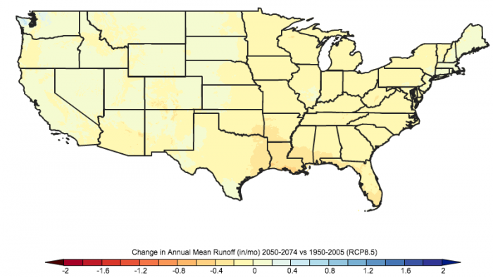
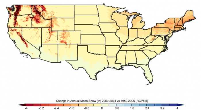
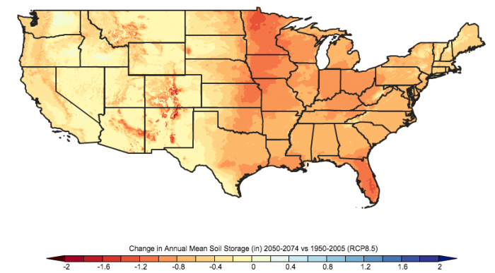
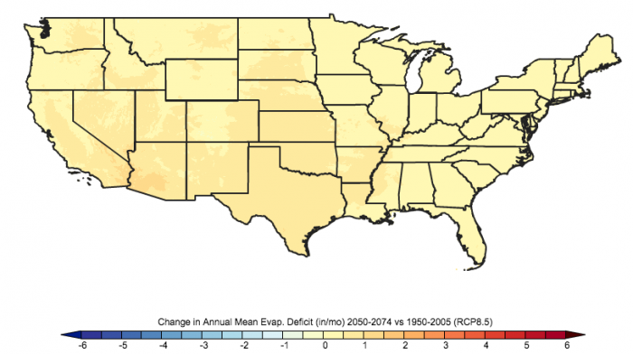
The Role of Our Food Systems in Climate Change
The Role of Our Food Systems in Climate Change
Food systems, including agriculture, play a significant role in contributing to global warming, perhaps contributing between 19% to 29% of global anthropogenic greenhouse gas emissions (Vermeulen et al. 2012). Growing food requires energy. While the sun is the source of energy for plant growth, a majority of the energy that fuels our modern food system comes from fossil fuels (petroleum and natural gas). Petroleum is used as a fuel for tractors and other vehicles that transport food. Natural gas is used in fertilizer production and other fossils fuels are burned to generate electricity that is used in the processing and refrigeration of food. The burning of fossil fuels is our largest source of greenhouse gases globally, and food production is a significant contributor to greenhouse gases.
The Food And Agriculture Organization of the United Nations (FAO) estimates that “the food sector (including input manufacturing, production, processing, transportation marketing and consumption) accounts for around 95 exa-Joules (1018 Joules), ...— approximately 30 percent of global energy consumption — and produces over 20 percent of global greenhouse gas emissions” (from Food and Agriculture Organization of the United Nations [89]).
In addition to carbon dioxide emissions from the fossil fuel consumption associated with agricultural activities discussed above, agriculture also contributes to greenhouse gas emissions in other ways (Figure 9.1.18). The loss of above-ground vegetation when grasslands and forests are converted to agriculture contributes about six percent of the global warming potential from greenhouse gas emissions. In addition, methane released from irrigated agriculture and from digestion and decomposition of manure from ruminants combined with nitrous oxide emissions from mismanagement of fertilizers contributes about 14 percent of the increase in total warming potential (Nelson 2014).
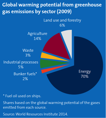
Module 9.2: Food Production in a Changing Climate
Module 9.2: Food Production in a Changing Climate
In Module 9.1, we explored the causes of global climate change, the ways that our food systems contribute to greenhouse gas emissions, and how climate variables are expected to change in different parts of the US. In this unit, we’ll consider the expected impacts of global climate change on food production.
Farmers have always had to struggle against the vagaries of the weather in their efforts to produce food for a growing population. Floods, droughts, heatwaves, hailstorms, late frosts, and windstorms have plagued farmers for centuries. However, with increased levels of CO2 in the atmosphere trapping more heat energy, farmers will face more extreme weather events, greater variability, and more extreme temperatures. Unpredictable and varied weather can lead to a domino effect through the entire food system, creating shortages and food price spikes. Farmers are developing strategies for resilience in the face of a changing climate, such as, more efficient irrigation, better soil health, and planting more resilient crop varieties.
Climate change can have both direct and indirect impacts on agricultural food production. Direct effects stem directly from changes in temperature, precipitation, and CO2 concentrations. For example, as temperatures increase in crop water demands and stresses on livestock increase. Changes in the maximum number of consecutive dry days can affect crop productivity. Increases in precipitation can increase soil erosion. Increased incidence of extreme weather events can also have direct impacts on agriculture, in the form of floods, droughts, hail and high winds.
Indirect effects of climate change include changes in weed, disease, and insect populations and distributions, which will have impacts on costs of managing pests and may increase crop losses. Increased incidence of wildfire can favor survival on invasive species. Some weeds respond well to increasing CO2 concentrations and may put greater pressure on crops.
In summary, a 2015 report on Climate Change, Global Food Security, and the U.S. Food System states that by 2050, global climate change may result in decreased crop yields, increased land area in crop production, higher food prices, and slightly reduced food production and consumption, compared to model results for 2015 with no climate change (Brown et al. 2015).
Global Effects of Climate Change
Human influences will continue to alter Earth’s climate throughout the 21st century. Current scientific understanding, supported by a large body of observational and modeling results, indicates that continued changes in the atmospheric composition will result in further increases in global average temperature, changes in precipitation patterns, rising sea level, changes in weather extremes, and continued declines in snow cover, land ice, and sea ice extent, among other effects that will affect U.S. and global agricultural systems.
While climate change effects vary among regions, among annual and perennial crops, and across livestock types, all production systems will be affected to some degree by climate change. Temperature increases coupled with more variable precipitation will reduce crop productivity and increase stress on livestock production systems. Extreme climate conditions, including dry spells, sustained droughts, and heatwaves will increasingly affect agricultural productivity and profitability. Climate change also exacerbates indirect biotic stresses on agricultural plants and animals. Changing pressures associated with weeds, diseases, and insect pests, together with potential changes in timing and coincidence of pollinator lifecycles, will affect growth and yields. When occurring in combination, climate change-driven effects may not simply be additive, but can also amplify the effects of other stresses on agroecosystems.
From Expert Stakeholder Workshop for the USDA Technical Report on Global Climate Change, Food Security, and the U.S. Food System [90]
Brown, M., P. Backlund, R. Hauser, J. Jadin, A. Murray, P. Robinson, and M. Walsh
June 25-27, 2013, Reston, VA,
Brown, M.E., J.M. Antle, P. Backlund, E.R. Carr, W.E. Easterling, M.K. Walsh, C. Ammann, W. Attavanich, C.B. Barrett, M.F. Bellemare, V. Dancheck, C. Funk, K. Grace, J.S.I. Ingram, H. Jiang, H. Maletta, T. Mata, A. Murray, M. Ngugi, D. Ojima, B. O’Neill, and C. Tebaldi. 2015. Climate Change, Global Food Security, and the U.S. Food System [91]. 146 pages.
Climate Variables that Affect Agriculture
Climate Variables that Affect Agriculture
In the first part of this module, we looked at observed and predicted changes in temperature and precipitation. Now, we'll consider some of the impacts that changes in temperature and precipitation may have on crops. For example, the projected increase in temperature will increase the length of the frost-free season (the period between the last frost in the spring and the first frost in the fall), which corresponds to a similar increase in growing season length. Increases in frost-free season length have already been documented in the US (Figure 9.2.1). An increase in growing season length may sound like a great thing for food production, but as we'll see, that can make plants more vulnerable to late frosts and can also allow for more generations of pests per growing season, thus increasing pest pressure. The complexity of the system makes adapting to a changing climate quite challenging, but not insurmountable.
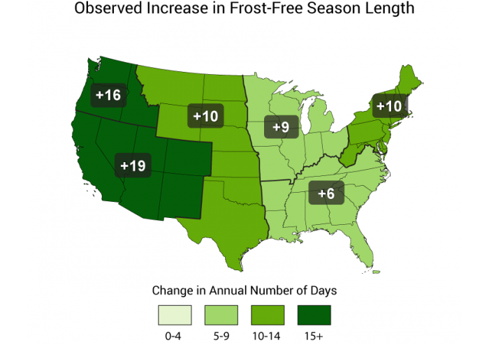
Crops, livestock, and pests are all sensitive to temperature and precipitation, so changes in temperature and precipitation patterns can affect agricultural production. As a result, it's important to consider future projections of climate variables so that farmers and ranchers can adapt to become more resilient.
Projected changes in some key climate variables that affect agricultural productivity are shown in Figure 9.2.2. The lengthening of the frost-free or growing season and reductions in the number of frost days (days with minimum temperatures below freezing), shown in the top two maps, can have both positive and negative impacts. With higher temperatures, plants grow and mature faster, but may produce smaller fruits and grains and nutrient value may be reduced. If farmers can adapt warmer season crops and planting times to the changing growing season, they may be able to take advantage of the changing growing season.
The bottom-left map in Figure 9.2.2 shows the expected increase in the number of consecutive days with less than 0.01 inches of precipitation, which has the greatest impact in the western and southern part of the U.S. The bottom-right map shows that an increase in the number of nights with a minimum temperature higher than 98% of the minimum temperatures between 1971 and 2000 is expected throughout the U.S., with the highest increase expected to occur in the south and southeast. The increases in both consecutive dry days and hot nights are expected to have negative effects on both crop and animal production. There are plants that can be particularly vulnerable at certain stages of their development. For example, one critical period is during pollination, which is very important for the development of fruit, grain or fiber. Increasing nighttime temperatures during the fruit, grain or fiber production period can result in lower productivity and reduced quality. Farmers are already seeing these effects, for example in 2010 and 2012 in the US Corn Belt (Hatfield et al., 2014).
Some perennial crops, such as fruit trees and grape vines, require exposure to a certain number of hours at cooler temperatures (32oF to 50oF), called chilling hours, in order for flowering and fruit production to occur. As temperatures are expected to increase, the number of chilling hours decreases, which may make fruit and wine production impossible in some areas. A decrease in chilling hours has already occurred in the Central Valley of California and is projected to increase up to 80% by 2100 (Figure 9.2.3). Adaptation to reduced chilling hours could involve planting different varieties and crops that have lower chilling hour requirements. For example, cherries require more than 1,000 hours, while peaches only require 225. Shifts in the temperature regime may result in major shifts in certain crop production to new regions (Hatfield et al., 2014).
To supplement our coverage of the climate variables that affect agriculture, read p. 18, Box 4 in Advancing Global Food Security in the Face of a Changing Climate [93], and scroll down to the Learning Checkpoint below.
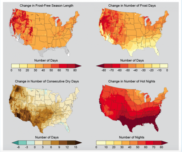
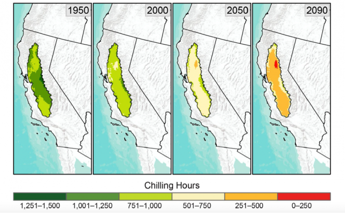
Learning Checkpoint
What are some of the challenges that farmers will face in a changing climate?
Click for the answer.
- increased temperatures
- leads to increased ET - increased water needs for the same crop production and increased water needs for irrigation
- heat stress
- can lead to reduced crop yields
- change in timing and intensity of rainfall
- more extreme weather events – floods and droughts
- increased CO2 concentrations
- may benefit some crops and weeds
- may negatively affect the nutritional makeup of some crops
- shifting zones of crop production
- changing threats from pests, disease, and invasive species
- insects
- weeds
In the first part of this module, we explored some maps from the National Climate Change Viewer. Discuss how the predicted changes in climate that you saw in those maps (Module 9.1 Projected Climate Changes [94]) will likely affect farmers.
Click for the answer.
Direct Effects of Climate Change on Crops
Direct Effects of Climate Change on Crops
Plants, whether crops or native plant species have adapted to flourish within a range of optimal temperatures for germination, growth, and reproduction. For example, plants at the poles or in alpine regions are adapted to short summers and long, cold winters, and so thrive within a certain range of colder temperatures. Temperature plays an important role in the different biological processes that are critical to plant development. The optimum temperature varies for germination, growth, and reproduction varies and those optimum temperatures needed to occur at certain times in the plant's life cycle, or the plant's growth and development may be impaired.
Let's consider corn as an example. In order for a corn seed to germinate, the soil temperature needs to be a minimum of 50oF. Corn seed typically will not germinate if the soil is colder than about 50oF. The minimum air temperature for vegetative growth (i.e., the growth of stem, leaves, and branches) is about 46oF, but the optimum range of temperatures for vegetative growth of corn is 77-90oF. At temperatures outside of the optimal range, growth tends to decline rapidly. Many plants can withstand short periods of temperatures outside of the optimal range, but extended periods of high temperatures above the optimal range can reduce the quality and yield of annual crops and tree fruits. The optimal reproduction of corn occurs between 64 and 72oF, and reproduction begins to fail at temperatures above 95oF. Reproductive failure for most crops begins around 95oF.
Water availability is a critical factor in agricultural production. We saw in Module 4 how increased temperature leads to increased transpiration rates. High rates of transpiration can also exhaust soil water supplies resulting in drought stress. Plants respond to drought stress through a variety of mechanisms, such as wilting their leaves, but the net result of prolonged drought stress is usually reduced productivity and yield. Water deficit during certain stages of a plant's growth can result in defects, such as tougher leaves in kales, chards, and mustards. Another example, blossom end rot in tomatoes and watermelon, is caused by water stress and results in fruit that is unmarketable (Figure 9.2.4 and for more photos of blossom end rot on different vegetables, visit Blossom end rot causes and cures in garden vegetables [95]).
In addition to water stress and impacts on plant productivity and yield, increased temperatures can have other effects on crops. High temperatures and direct sunlight can sunburn developing fruits and vegetables. Intense heat can even scald or cook fruits and vegetables while still on the plant.
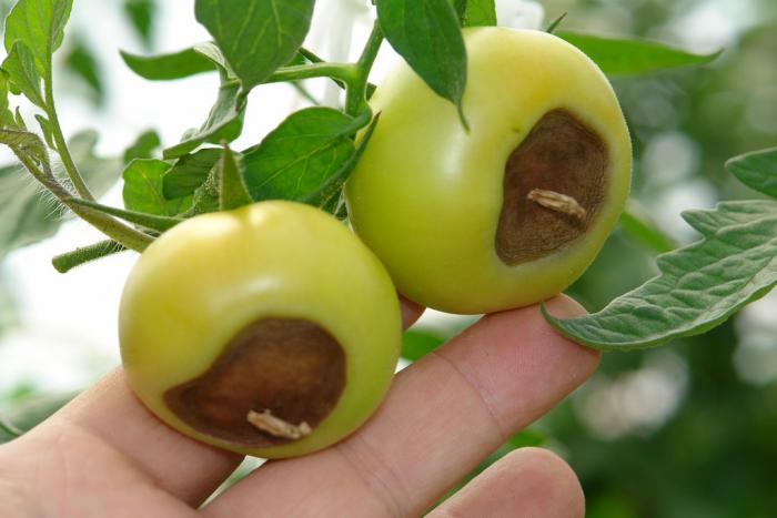
(NRCS_Photo_Gallery).jpg)
Crop yield
A warming climate is expected to have negative impacts on crop yields. Negative impacts are already being seen in a few crops in different parts of the world. Figure 9.2.5 shows estimated impacts of climate trends on crop yields from 1980-2008, with declines exceeding 5% for corn, wheat, and soy in some parts of the world. Projections under different emissions scenarios for California's Central Valley show that wheat, cotton, and sunflower have the largest declines in yields, while rice and tomatoes are much less affected (Figure 9.2.6). Notice that there are two lines on the graphs in Figure 9.2.6 projecting crop yields into the future. The red line corresponds to temperature increases associated with a higher carbon dioxide emissions scenario. We saw in Module 9.1 that the more CO2 we emit, the more heat energy is trapped in the lower atmosphere, and therefore the warmer the temperatures. For some crops, those higher temperatures are associated with great impacts on the crop's yield.
Why are some crops affected more by observed and projected temperature increases than others? It depends on the crop, the climate in the region where the crop is being grown, and the amount of temperature increase. Consider the Activate your learning questions below to explore this more deeply.
Why do some crops see a positive yield change with increasing temperatures, such as alfalfa in Figure 9.2.6? Generally, warmer temperatures mean increased crop productivity, as long as those temperatures remain within the optimal range for that crop. If a crop is being grown in a climate that has typical temperatures at the cooler end of the plant's optimal range, than a bit of warming could increase the crop's productivity. If the temperatures increase above the optimal range or exceed the temperature that leads to reproductive failure, then crop yields will decline.
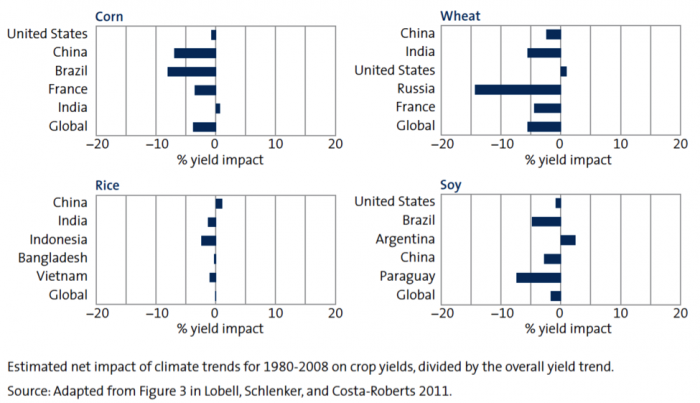
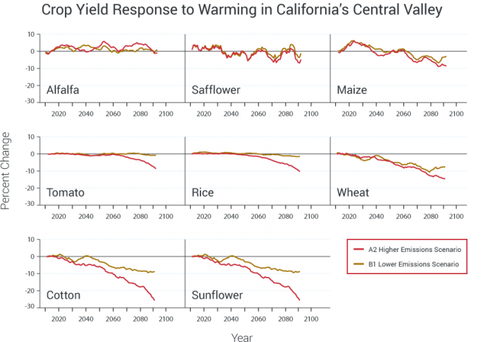
Activate your learning
Inspect Figure 9.2.5 above. Which crops' yields have already been most affected by climate change, and which crops the least?
Click for the answer.
What are some possible reasons for the difference in yield impact between corn, wheat, and rice that you see in Figure 9.2.5?
Click for the answer.
Consider the graph for Wheat in Figure 9.2.5. What is the % yield impact in Russia and United States? What could cause differences in yield impact between regions?
Click for the answer.
Indirect Effects of Climate Change on Plants
Indirect Effects of Climate Change on Plants
Weeds, Insects, and Diseases
Warming temperatures associated with climate change will not only have an effect on crop species; increasing temperature also affects weeds, insect pests, and crop diseases. Weeds already cause about 34% of crop losses with insects causing 18% and disease 16%. Climate change has the potential to increase the large negative impact that weeds, insects, and diseases already have on our agricultural production system. Some anticipated effects include:
- several weed species benefit more than crops from higher temperatures and increased CO2 levels
- warmer temperatures increase insect pest success by accelerating life cycles, which reduces time spent in vulnerable life stages
- warmer temperatures increase winter survival and promote the northward expansion of a range of insects, weeds, and pathogens
- longer growing seasons allow pest populations to increase because more generations of pests can be produced in a single growing season
- temperature and moisture stress associated with a warming climate leaves crops more vulnerable to disease
- changes in disease prevalence and range will also affect livestock production
Modeling and predicting the rate of change and magnitude of the impact of weeds, insects, and disease on crops is particularly challenging because of the complexity of interactions between the different components of the system. The agricultural production system is complex and the interactions between species are dynamic. Climate change will likely complicate the management of weeds, pests, and diseases as the ranges of these species changes.
Effects on Soil Resources
The natural productive capacity of a farm or ranch system relies on a healthy soil ecosystem. Changing climate conditions, including extremes of temperature and precipitation, can damage soils. Climate change can interfere with healthy soil life processes and diminish the ecosystem services provided by the soil, such as the water holding capacity, soil carbon, and nutrients provided by the soils.
The intensity and frequency of extreme precipitation events are already increasing and is expected to continue to increase, which will increase soil erosion in the absence of conservation practices. Soil erosion occurs when rainfall exceeds the ability of the soil to absorb the water by infiltration. If the water can't infiltrate into the soil, it runs off over the surface and carries topsoil with it (Figure 9.2.7). The water and soil that runoff during extreme rainfall events are no longer available to support crop growth.
Shifts in rainfall patterns associated with climate change are projects to produce more intense rainstorms more often. For example, there has been a large increase in the number of days with heavy rainfall in Iowa (Figure 9.2.8), despite the fact that total annual precipitation in Iowa has not increased. Soil erosion from intense precipitation events also results in increased off-site sediment pollution. Maintaining some cover on the soil surface, such as crop residue, mulch, or cover crops, can help mitigate soil erosion. Better soil management practices will become even more important as the intensity and frequency of extreme precipitation increases.
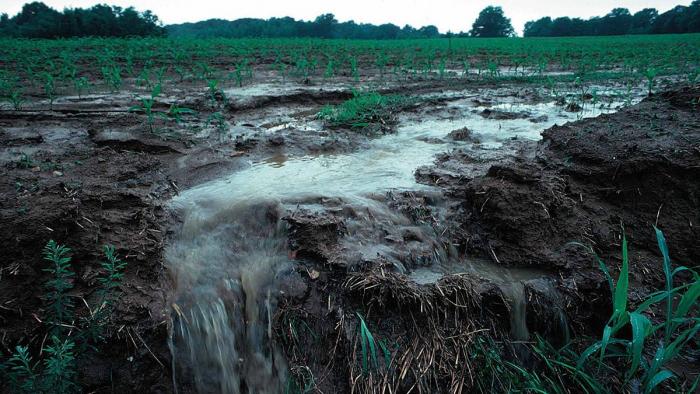
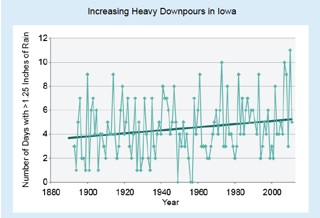
How Farmers Adapt to Climate Change
How Farmers Adapt to Climate Change
Farmers have had to adapt to the conditions imposed on them by the climate of their region since the inception of agriculture, but recent human-induced climate change is throwing them some unexpected curve balls. Extreme heat, floods, droughts, hail, and windstorms are some of the direct effects. In addition, there are changes in weed species and distribution, and pest and disease pressures, on top of potentially depleted soils and water stress. Fortunately, there are many practices that farmers can adopt and changes that can be made to our agricultural production system to make the system more resilient to our changing climate.
Farmers and ranchers are already adapting to our changing climate by changing their selection of crops and the timing of their field operations. Some farmers are applying increasing amounts of pesticides to control increased pest pressure. Many of the practices typically associated with sustainable agriculture can also help increase the resilience of the agricultural system to impact of climate change, such as:
- diversifying crop rotations
- integrating livestock with crop production systems
- improving soil quality
- minimizing off-farm flows of nutrients and pesticides
- implementing more efficient irrigation practices
The video below introduces and discusses several strategies being adopted by New York farmers to adapt to climate change. In addition, the fact sheet from Cornell University's Cooperative Extension about Farming Success in an Uncertain Climate [98]produced by Cornell University's Cooperative Extension outlines solutions to challenges associated with floods, droughts, heat stress, insect invasions, and superweeds. Also, p. 35, Box 8 in Advancing Global Food Security in the Face of a Changing Climate [93] outlines some existing technologies that can be a starting point for adapting to climate change.
Learning Checkpoint: How can farmers adapt to climate change?
- Watch 15 min video by Cornell University about Agriculture and Adaptation about how New York farmers are adapting to climate change.
- Read the fact sheet from Cornell University's Cooperative Extension about Farming Success in an Uncertain Climate [98]
- Read p. 35, Box 8 in Advancing Global Food Security in the Face of a Changing Climate [93]
- Answer the questions below
Video: Climate Smart Farming Story: Adaptation and Agriculture (15:09)
Check Your Understanding
How can frost damage increase with climate change, even if temperatures are overall warming?
Click for the answer.
What are some ways that the risk of frost damage can be reduced in a warming climate?
Click for the answer.
Why is triticale a beneficial forage crop for farmers to grow?
Click for the answer.
What is an important management strategy that farmers can use in growing grapes to work with a changing climate?
Click for answer.
What climate change impacts are the farmers in the video dealing with?
Click for answer.
What strategies are implemented by the farmers in the video to manage their farms in a changing climate?
Click for the answer.
References:
- Hatfield, J., G. Takle, R. Grotjahn, P. Holden, R. C. Izaurralde, T. Mader, E. Marshall, and D. Liverman, 2014: Ch. 6: Agriculture. Climate Change Impacts in the United States: The Third National Climate Assessment, J. M. Melillo, Terese (T.C.) Richmond, and G. W. Yohe, Eds., U.S. Global Change Research Program, 150-174. doi:10.7930/J02Z13FR. On the Web: http://nca2014.globalchange.gov/report/sectors/agriculture [99]
- Lengnick, L. 2015. Resilient Agriculture: Cultivating Food Systems for a Changing Climate, New Society Publishers.
Climate Change in the Coupled Human-Natural System
Climate Change in the Coupled Human-Natural System
We've covered quite a bit of ground in this module. We explored how human activities have led to an increase in atmospheric carbon dioxide, which in turn is increasing the surface temperature of the Earth and changing precipitation patterns. The resulting impacts on our agricultural production system are complex and potentially negative. As a result, farmers are adopting new practices and technologies to adapt to our changing climate and create more resiliency in the agricultural system.
Let's put global climate change and its interaction with our agricultural system into the Coupled Human-Natural System (CHNS) diagram that we've been using throughout the course. The development of global climate change is illustrated in the CHNS diagram in Figure 9.2.9, where the increased burning of fossil fuels within the human system results in more CO2 in the atmosphere. The response in the natural system is that more heat energy is trapped. The resulting feedback that affects the human system is that temperature increases along with all of the other climate change effects that we discuss in this module.
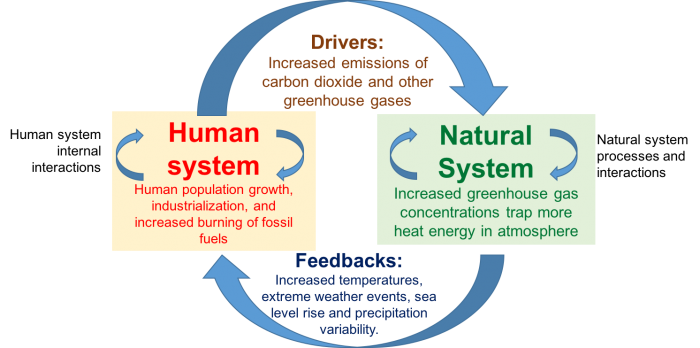
This loop shows the human system with an arrow labeled drivers pointing to natural system with an arrow labeled feedbacks pointing back to human system. Those four concepts are defined as follows:
Human system (human system internal interactions): human population growth, industrialization, and increased burning of fossil fuels
Drivers: increased emissions of carbon dioxide and other greenhouse gases
Natural system (natural system processes and interactions): increased greenhouse gas concentrations trap more heat energy in atmosphere
Feedbacks: increased temperatures, extreme weather events, sea level rise and precipitation variability
What would be the next step in the diagram? Consider the feedbacks associated with the arrow at the bottom of the diagram that will affect the human system. What are the possible responses in the human system to these feedbacks? Our response can be categorized into two broad categories: mitigation and adaptation. We've already discussed adaptation strategies that can be implemented by farmers to adapt to a changing climate. Some examples are to change the crops grown to adapt to the higher temperatures or to install more efficient irrigation systems so that crops can be grown more efficiently.
What about mitigation? Mitigation strategies are those that are targeted at reducing the severity of climate change. One important mitigation strategy is to reduce the burning of fossil fuel, and our agricultural system is a significant contributor to greenhouse gas emissions. Shifting to use renewable energy sources and more fuel-efficient equipment are two mitigation strategies. There are other important mitigation strategies that target other greenhouse gas emissions, such as nitrous oxide from fertilizer use and methane from ruminants and some types of irrigated agriculture.
In the next couple of modules, we'll talk more about strategies to make our agricultural systems more resilient and sustainable, and you'll see how our food production can become more resilient to climate change. In addition, you'll get the opportunity to explore the project climate change impacts on your capstone region and to consider how those projected change might affect the food systems of that region.
Summative Assessment: Climate Change Predictions in your Capstone Region
Summative Assessment: Climate Change Predictions in your Capstone Region
Summary
The summative assessment for Module 9 involves exploring the predictions of future climate variables from climate models for the US, then considering the possible impacts of increased temperature on your capstone region. Also, you will propose strategies to increase the resilience of the food systems in your capstone region to increasing temperatures.
The summative assessment for this module has two parts:
- Exploration of the National Climate Change Viewer - view national predicted change in climate variables for the US
- Data collection and interpretation from the National Climate Change Viewer for your capstone region
The second part requires that you work on the data collection for Stage 3 of the capstone project. Your grade for the module summative assessment will be based on your answers to the questions in the worksheet, which you will answer using the data you download and organize for the capstone.
For the capstone project, you will need to consider the resilience and vulnerabilities of the food systems in your assigned region to projected increases in temperatures. Your task now is to determine what are the temperature increases projected in your assigned region as a result of human-induced climate change. Also, you'll need to start thinking about what impacts those changes may have on the food system in your region. You'll use the National Climate Change Viewer (NCCV) to explore predicted changes in climate variables for the US and to investigate the projected changes in minimum and maximum monthly temperatures in your assigned region.
Instructions
Download the worksheet linked on the next page.
Submitting Your Assignment
Type your answers in essay format into the provided worksheet. If you can, highlight your answers. Submit your document to Module 9 Summative Assessment in Canvas.
Grading Information and Rubric
Your assignment will be evaluated based on the following rubric. The maximum grade for the assignment is 35 points. Pay very close attention to this rubric. The final questions on the worksheet are worth the most points!
| Criteria | Possible Points |
|---|---|
| 1. Summary of projected changes in climate demonstrates a clear understanding of the data retrieved from the NCCV. Correct units of measure are used in the discussion of climate variables. | 10 |
| 2. Summary of climate change impacts on crops shows that the students understand basic connections between plants growth and climate variables. | 10 |
| 3. The answer demonstrates that students considered the adaptation strategies presented in this module and identified strategies appropriate for the regions, including consideration of the region's crops, climate, and food systems. | 10 |
| Answers are typed and clearly and logically written with no spelling and grammar errors | 5 |
Summary and Final Tasks
Summary
In Module 9, we covered the human activities that have led to climate change and the resulting impacts on global climate. We explored some of the climate variables that will affect agriculture and then considered possible adaptation strategies that can be employed to make agriculture more resilient to climate change.
In the next two modules, we will delve deeper into the complexity of the coupled human-natural food system, continuing to employ spatial thinking. In Module 11, we will explore strategies to make food systems more resilient and sustainable. In order, to do that though we need to understand how vulnerable those systems are to stressors like climate change, and to identify the adaptive capacity of those systems. In that final module before the capstone, many of the concepts covered in the course will come together.
Finally, your capstone data collection should be proceeding. The Summative Assessment for Module 9 required that you capture some critical information for your capstone region. The data gathered about projected temperature changes in your capstone region is integral to your final assessment of the resilience of the food systems in your capstone region.
Reminder - Complete all of the Module 9 Tasks!
You have reached the end of Module 9. Double-check the to-do list on the Module 9 Roadmap [100] to make sure you have completed all of the activities listed there before you begin Module 10.
References and Further Reading
Cornell University, College of Agriculture and Life Sciences, Climate Change Facts, 2013, Farm Energy, Carbon, and Greenhouse Gases, (https://cpb-us-e1.wpmucdn.com/blogs.cornell.edu/dist/8/4308/files/2015/0... [101])
Cornell University, College of Agriculture and Life Sciences, Climate Change Facts, 2013, Farming Success in an Uncertain Climate [102](https://ecommons.cornell.edu/bitstream/handle/1813/54950/CornellClimateC... [102])
Hatfield, J., K. Boote, P. Fay, L. Hahn, C. Izaurralde, B.A. Kimball, T. Mader, J. Morgan, D. Ort, W. Polley, A. Thomson, and D. Wolfe, 2008. Agriculture. In: T [103]he effects of climate change on agriculture, land resources, water resources, and biodiversity [103]. A Report by the U.S. Climate Change Science Program and the Subcommittee on Global Change Research. Washington, DC., USA, 362 pp. (CCSP_Ag_Report.pdf from http://www.sap43.ucar.edu/documents/Agriculture.pdf [104])
Hatfield, J., G. Takle, R. Grotjahn, P. Holden, R. C. Izaurralde, T. Mader, E. Marshall, and D. Liverman, 2014: Ch. 6: Agriculture. Climate Change Impacts in the United States: The Third National Climate Assessment [105], J. M. Melillo, Terese (T.C.) Richmond, and G. W. Yohe, Eds., U.S. Global Change Research Program, 150-174. doi:10.7930/J02Z13FR. (NCA3_Full_Report_06_Ag.pdf from http://nca2014.globalchange.gov/report/sectors/agriculture [99])
Lengnick, L., 2015, Resilient Agriculture: Cultivating Food Systems for a Changing Climate, New Society Publishers, 288 pp.
Nelson, G.C., 2014, Advancing Global Food Security in the Face of a Changing Climate [93], The Chicago Council on Global Affairs.
Vermeulen, S.J., B.M. Campbell, J.S.I. Ingram, 2012, Climate Change and Food Systems, Annual Review of Environmental Resources [106], Vol. 37: 195-222. (Vermeulen_etal_2012_ClimateChangeFoodSystems.pdf from http://www.annualreviews.org/doi/pdf/10.1146/annurev-environ-020411-130608 [107] )
Capstone Project Stage 3 Assignment
Capstone Project Stage 3 Assignment
Soil/Crop Management, Pests, and Climate Change
(Modules 7-9)
At this stage, you should have collected quite a bit of data related to the physical environment of your region (water, soils, and climate) as well as related to the regional food system, including the history of the regional food system and which crops are grown in your region. You may also have discovered some impacts that the regional food system is having on soil and water resources in the region.
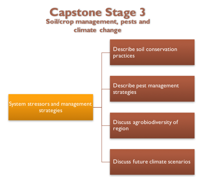
- System stressors and management strategies
- describe soil conservation practices
- describe pest management strategies
- discuss agrobiodiversity of region
- discuss future climate scenarios
What to do for Stage 3?
- Download and complete the Capstone Project Stage 3 worksheet [108] that contains a table summarizing the data you’ll need to collect to complete this stage. Remember, you need to think deeply about each response and write responses that reflect the depth of your thought as informed by your research.
- Add questions and continue to research the questions in your worksheet files.
- Keep track of all of the resources and references you use.
- Add relevant data, maps, and figures to your PowerPoint file.
- Revise your CHNS diagram and/or create a new one incorporating topics from Modules 7, 8 and 9.