Lesson 6: Validation of Imagery and Elevation Data
Lesson 6 Introduction
Lesson 6 provides an overview of accuracy assessment procedures and standards applied to remotely sensed mapping datasets intended for public use in the United States. In the context of this lesson, accuracy assessment refers primarily to geometric fidelity of the dataset, the degree to which the spatial coordinates of a data element agree with their “true” coordinates on the earth’s surface. However, in reference to image analysis, accuracy assessment also refers to the correctness of the thematic maps produced by land cover classification or change detection. Geometric accuracy is the focus of this lesson; classification accuracy is discussed in depth in Geography 883.
Accuracy assessment is a quantitative analysis of the spatial correctness of the dataset compared to the surface it represents. For most mapping products, there are also aesthetic standards for elements of quality which may not affect spatial accuracy, but can either enhance or detract from the experience of viewing the data or using it as a backdrop in GIS. The lesson material will focus on quantitative methods of accuracy assessment, but, for completeness, will also touch upon the qualitative. Together, the quantitative and qualitative evaluations are referred to by the broader terms, quality assurance and quality control (QA/QC).
A number of accuracy standards, used by public agencies and many private entities throughout the United States, will be presented in the textbook readings and summarized in the online course material. The study of standards and data specifications demands concern for minute details and precise use of terms and definitions. In this course, we have not been able to study all of the detailed elements of remote sensing technology and datasets addressed by most mapping standards; therefore, it’s important to try to get an overall sense of the major categories of issues being addressed. By the end of this lesson, the student should have an appreciation for the way remote sensing datasets are evaluated for geometric accuracy, and the way the results of those evaluations are (or at least, should be) reported to end users.
Lesson Objectives
At the end of this lesson, you will be able to:
- describe and compare various federal and state standards for imagery and elevation data;
- compute a quantitative accuracy assessment in accordance with FGDC standards;
- perform visual quality assessment for both imagery and elevation data.
Questions?
If you have any questions now or at any point during this week, please feel free to post them to the Lesson 6 Questions and Comments Discussion Forum in Canvas.
Definitions
The terms quality control and quality assurance are often used somewhat interchangeably, or in tandem, to refer to a multitude of tasks performed internally by the data producer and externally, or independently, by the data purchaser. For the purposes of this course, we will adopt the following definitions provided in Maune (2007):
Quality Assurance (QA) –
Steps taken: (1) to ensure the end client receives the quality products it pays for, consistent with the Scope of Work, and/or (2) to ensure an organization’s Quality Program works effectively. Quality Programs include quality control procedures for specific products as well as overall Quality Plans that typically mandate an organization’s communication procedures, document and data control procedures, quality audit procedures, and training programs necessary for delivery of quality products and services.Quality Control (QC) –
Steps taken by data producers to ensure delivery of products that satisfy standards, guidelines, and specifications identified in the Scope of Work. These steps typically include production flow charts with built-in procedures to ensure quality at each step of the work flow, in-process quality reviews, and/or final quality inspections prior to delivery of products to a client.Independent QA/QC –
Steps taken by a QA/QC specialty firm, hired by the client (e.g., government or data producer) to independently validate the effectiveness of the data producer’s quality processes.
Quantitative accuracy assessment (testing remotely sensing mapping products against ground control checkpoints) falls under the category of independent QA/QC defined above. It is normally conducted by an individual or organization that had no involvement in the data acquisition or production. The ground check points are not made available to the data producer; so that the final coordinate comparison is truly an independent test of spatial accuracy.
Before we delve further into the topic of accuracy assessment, we must define exactly what we mean when we use the term "accuracy" and distinguish it from the related term, "precision."
Absolute accuracy -
Absolute accuracy is the closeness of an estimated, measured, or computed value to a standard, accepted, or true value of a particular quantity. In mapping, a statement of absolute accuracy is made with respect to a datum, which is, in fact, also an adjustment of many measurements and has some inherent error. The statement of absolute accuracy is made with respect to this reference surface, assuming it is the true value.Relative accuracy -
Relative accuracy is an evaluation of the amount of error in determining the location of one point or feature with respect to another. For example, the difference in elevation between two points on the earth's surface may be measured very accurately, but the stated elevations of both points with respect to the reference datum could contain a large error. In this case, the relative accuracy of the point elevations is high, but the absolute accuracy is low.Precision -
Precision is a statistical measure of the tendency for independent, repeated measurements of a value to produce the same result. A measurement can be highly repeatable, therefore very precise, but inaccurate if the measuring instrument is not calibrated correctly. The same error would be repeated precisely in every measurement, but none of the measurements would be accurate.
Independent check points are used to assess the absolute accuracy of a remotely-sensed dataset. Realize, however, that the check point coordinates are also derived from some form of surveying measurement, and there is also some degree of error associated with them. It is customary to require that the check points be at least three times as accurate as the targeted accuracy of the mapping product being tested; for example, if an orthophoto product is specified to have no more than 1 foot of horizontal error, then the check points used to test the orthophoto product should themselves contain no more than 1/3 foot of error.
As you will learn in this lesson, quantification of error and accuracy relies on statistical principles of probability. Accuracy standards for imagery and terrain data are described in probabilistic terms; for example, one might report that the coordinates of an object derived from an orthophoto image were tested against independent ground checkpoints and were shown to agree within certain number of feet at the 90% or 95% percent confidence level. Confidence level refers to the probability that any other independently tested point in the dataset will differ from its true value by no more than the stated amount.
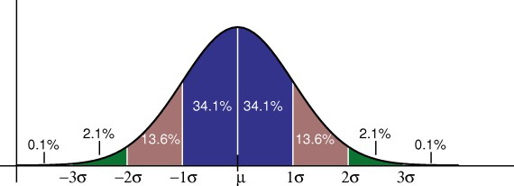
The statistical model used to determine this confidence level is most often the normal, or Gaussian, distribution [1]. The assumption underlying the use of this statistical model is that the errors associated with repeated measurements of the same physical quantity will distribute themselves according to a particular probability density function, the Gaussian "bell curve," shown below in Figure 1. Measurements very close to the true value are the most likely, but measurements that deviate from the true value will occur on a less frequent, yet predictable, basis. The peak of the bell curve represents the mean of all measurements and the true value of the variable in question; the sloping sides of the curve represent the probability of observing values that deviate from the mean. In a normal distribution, the deviations must be distributed symmetrically about the mean; in other words, high values are as likely as low values. The width of the curve represents the range of probable values with respect to the true value, or the magnitude of probable error.
The statistical parameter used to quantify the width of the Gaussian bell curve is the standard deviation, known as sigma, also often referred in the GIS world to as the root-mean-square-error (RMSE). Given a large enough sample of measurements, 68% will fall within one sigma of the mean, 95% will fall within about two sigma (1.96*sigma, to be precise), and 99.8% will fall within three sigma. When comparing a spatial dataset to a sample of ground checkpoints, one can plot the differences between the observed coordinates and the checkpoint coordinates, compute the mean error and RMSE using standard statistical formulas, and report accuracy at the 95% confidence limit as a function of RMSE.
Remember that the basic assumption one makes when applying the normal distribution as an appropriate error model is that there are no irregularities or artifacts in the data that would cause the actual error distribution to differ from the ideal Gaussian bell curve. Furthermore, for RMSE to apply as a statement of absolute positional accuracy, there can be no biases or systematic errors in the dataset that cause the average error to be significantly non-zero. Remotely sensed datasets may contain systematic errors, either due to characteristics of the sensor or characteristics of the target. In the lesson material to come, you will see examples of this, and you will see how the statistics used in accuracy assessment help to point out these biases and diagnose their cause.
Validation of Orthorectified Imagery
One of the first points to make in a discussion about spatial accuracy of orthorectified imagery is that accuracy is completely unrelated to spatial resolution. The size of a pixel has no physical bearing on the accuracy of its location in the ground coordinate system. Spatial accuracy depends only on the quality of the georeferencing, either as applied from ground control with aerotriangulation or provided by direct georeferencing. The difference between spatial accuracy and spatial resolution is often overlooked or unrecognized by the layman, and it is often not made clear to the uninitiated public consumer in marketing literature or by the news media.
The size of an object that can be seen in an image, compared to the accuracy of its location as derived from the image, may be significantly different. For example, the standard USGS and NAIP DOQQ products were produced at a 1-meter GSD with a targeted horizontal accuracy of about 10 meters at the 90% confidence level compared to ground surveyed checkpoints. When circumstances and budgets permit, it is desirable to specify a spatial accuracy requirement that is comparable to the size of a pixel in ground units. For example, if the output image pixel size is 1 meter, then the spatial accuracy requirement might be defined such that each 1-meter pixel in the image was assured to be within 2 meters of its "true" location in the ground coordinate system at the 95% confidence limit. The general rule of thumb is to target a root-mean-square-error (RMSE) for spatial accuracy equivalent to the size of a pixel (GSD) in the output image. In practice, and depending on the end user application, it is not always possible or necessary to follow this rule. If the primary purpose of the imagery is simply to identify objects and measure their size relative to each other, then the absolute spatial accuracy in terms of ground coordinates may be less important than relative accuracy or spatial resolution. If the objective is to create secondary map products from the orthorectified imagery, such as building footprints or road centerlines, then the absolute accuracy should be comparable to resolution.
In the interest of economy, some image data products are generated using control extracted from other image sources, rather than using new ground control or direct georeferencing data acquired along with the new imagery. This is akin to the exercise we performed in the final part of the Lesson 3 lab, using image points I provided as a source of control for orthorectification. Many USDA NAIP DOQQs use USGS DOQQs as a source of georeferencing control. Furthermore, they often use the USGS DOQQs as a source of "independent" check points; so that the accuracy that is reported is a comparison to the USGS image, not the actual ground. The following quote, consistent with USDA NAIP program specifications, is extracted from the metadata of the 2005 NAIP DOQQs for the state of Minnesota [5], "the source quarter-quad files are 2 meter ground sample distance (GSD) orthoimagery rectified to a horizontal accuracy of within 10 meters of reference digital orthophoto quarter quads (DOQQ's) from the National Digital Ortho Program (NDOP)." This is a statement of relative accuracy, not of absolute accuracy. One must read the metadata carefully to understand the distinction; relying on software, simply reading the RMSE from a metadata field, may lead to faulty assumptions about the spatial accuracy of the data one is using for analysis.
Data Validation
Acceptance of an orthorectified image deliverable should validate all the product specifications defined by the end user. There are three general categories of quality control and quality assurance checks and tests:
- Data Integrity - do the files contain what they are supposed to contain?
- Spatial Accuracy - do the data products meet the end user requirements for horizontal accuracy?
- Aesthetics - do the data products meet the customer's expectations in terms of color balancing, edge matching from photo to photo, and other general image quality characteristics?
Simply viewing the imagery in a GIS environment accomplishes the data integrity step. This cursory view can ensure that:
- individual image files are in the correct format and the files have not been corrupted;
- complete coverage of the area of interest has been achieved;
- accurate georeferencing information exists for each image file, in the specified coordinate system;
- size of image pixels matches the data product specification.
Quantitative Assessment
Orthorectified imagery is very often used as a visual backdrop to other GIS data or as a source for image interpretation and collection of point, line, or polygon features to be used in GIS. Because of this widespread use as a base map, quantitative accuracy assessment is one of the most important aspects of orthophoto quality assurance and acceptance testing.
An orthophoto is essentially a 2-dimensional product. As we learned in Lesson 3, the fidelity and accuracy of the terrain model used in the rectification process has an impact on the horizontal accuracy of the orthophoto; however, the image dataset has no elevation information contained explicitly within it. Horizontal accuracy is the only relevant spatial accuracy assessment metric. The end user's accuracy specification is commonly stated as a root-mean-square-error (RMSE) based on measurements of well-defined points in the imagery compared to independent survey measurements of higher accuracy serving as ground truth. The definition of a well-defined point, guidance on the selection and surveying of these checkpoints, and the methodology for calculating the RMSE is documented in the National Standard for Spatial Data Accuracy [6] (NSSDA) published by the US Federal Geographic Data Committee.
For historical reasons, mapping accuracies are commonly specified at the 95% confidence limit. A typical accuracy statement accompanying an orthophoto deliverable would be "Tested ____ (meters, feet) horizontal accuracy at 95% confidence level," and the numerical value supplied is RMSE * 1.7308. This statement of accuracy assumes that no systematic errors or biases are present in the data and that the individual checkpoint errors follow a normal distribution, independent in the x and y directions. Note that the multiplier for the RMSE is 1.7308, rather than the 1.96 factor stated in the Introduction page of this lesson. Horizontal error is a circular error, a combination of the independent linear errors in the x and y dimensions.
Most professional practitioners involved in the design of a remote sensing data acquisition know how to design a project to meet the designated accuracy specification. When errors exceed specification, there is usually a systematic cause. Common problems are instrument misalignment or miscalibration, georeferencing system drifts, and blunders in datum or coordinate system conversion. Systematic errors such as these can be detected by examining other statistical metrics and plotting the spatial distribution of the errors. In a dataset containing systematic errors, the mean of the errors will be non-zero and the entire may be shifted north, south, east, or west from its proper location. Systematic trends are easily detectable and can usually be related to a physical cause. Once the cause has been determined, systematic errors can often be corrected by reprocessing the data. Only when systematic errors have been successfully removed does the RMSE or 95% confidence statement give the user a true indication of the absolute accuracy of the data product.
The process of accuracy assessment begins with collection of a number of ground checkpoints, usually surveyed with GPS, accompanied by a set of field sketches and photographs to aid the image analyst in proper identification in the orthophoto image. Figure 2 shows an example of such a check point, chosen because it can be clearly and unambiguously identified in the orthophoto to be tested.
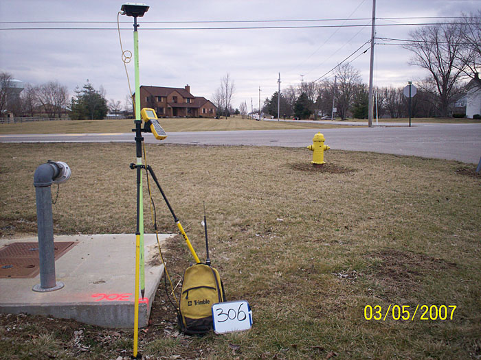
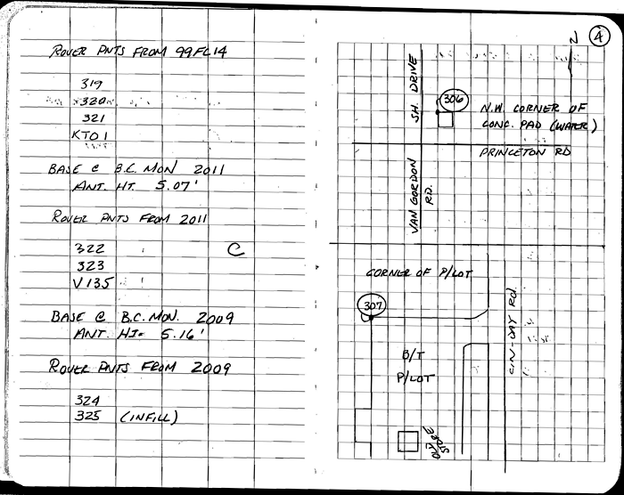
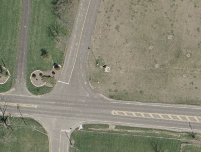
The survey sketch shown in Figure 3 above is an important complement to the digital photograph. The sketch provides additional information about the vicinity of the point that helps the image analyst navigate to the correct vicinity of the point. Armed with the surveyed coordinate derived GPS, the digital photo, and the field sketch, the image analyst should be able to locate the point within the project area, identify the correct orthophoto image within the project database to be examined, and navigate to the exact location of the point, as shown in Figure 4. The surveyed coordinates, derived from GPS, are then compared to the coordinate readout from the orthophoto in GIS or CAD software.
The image analyst visits and records the coordinates for each surveyed checkpoint in the orthophoto imagery. This can be done quite easily in GIS software. The survey results can be imported as a point file and overlaid on the orthophoto with identifying labels. The points should fall very close to the correct location, and the image analyst has only to confirm the exact location, using the photo and the sketch. The image point measurements are recorded in another point file. A table of coordinates can be exported from the GIS or CAD software and used to generate graphs and statistics, such as mean error in each direction, RMSE and 95% confidence values.
Qualitative Assessment
The final step of acceptance testing involves an examination of general image quality. The imagery for a large project may have been flown over a period of weeks under varying lighting conditions. Matching and balancing the brightness, contrast, and color tones may require use of image processing software.
The USDA developed a set of documents describing the type of visual artifacts they commonly see in orthophoto deliverables to the NAIP program. Because this type of visual inspection goes beyond the intended scope of this lesson, it won't be discussed in the lesson material. Feel free to review the referenced documents, which have been made available through the course download site. These are specific to a particular federal imagery program; however, the types of artifacts encountered and the image processing techniques recommended to overcome them can be widely applied.
- FSA User Sensitivity Study for Quality of National Agricultural Imagery Program (NAIP) Imagery [8] - Interim Technical Report looks at end user sensitivity to aesthetic issues, such as noise, sharpness, color registration, color saturation, color balance, and tonal variation. The report is a valuable example because it examines the impact of these issues in the context of the intended application. While aesthetic defects may be distracting or annoying from a purely aesthetic point of view, the prescribed remedy may not produce sufficient benefits to justify the cost or time required to implement.
- Aerial Photography Field Office-National Agriculture Imagery Program (NAIP) Suggested Best Practices [9] - Final Report provides guidelines and recommendations for the use of image processing techniques to effectively remedy defects identified in the User Sensitivity Study.
- Aerial Photography Field Office-Scaled Variations Artifact Book [10] provides a number of graphic examples of the defects before and after image processing remedies have been applied.
Validation of Elevation Data
The approach and methods for vertical accuracy testing of terrain data are very similar to those presented above for orthorectified imagery. Elevations are measured relative to a vertical datum, and the vertical datum itself is an approximation of something ideal such as “mean sea level,” which cannot be exactly and completely known, because it is by definition an average. We cannot say absolutely that a particular elevation is accurate to within 1 foot, 1 inch, or 1 millimeter of its true value. However, we can express the level of confidence we have in a measurement based on a framework of statistical testing. Based on a sample of independent elevation check points, we can say we have a level of confidence that any other point in the entire dataset is within the stated tolerance of its “true” value expressed relative to one vertical datum or another.
In this course, you have been introduced to the distinctly different technologies for capturing terrain data that have come into maturity in recent decades: photogrammetry, lidar, and IFSAR. Because these technologies are so new to both data providers and end users, the topic of QA/QC of terrain data has been the subject of much debate and study. Not only is there a high level of interest in applications that make use of terrain data, there is also a pervasive need to understand the strengths and weaknesses of each technology in order to make good investment decisions in equipment, software, and data.
As discussed above, the QA/QC process gives us insight into the types of errors and artifacts that affect terrain data, due either to the sensor or to characteristics of the target surface. With respect to the terrain data, there was concern from the start that vertical accuracy would vary within a single dataset, based on the type of terrain and land cover being mapped. In other words, there was some recognition that accuracy itself was a spatial variable. While this is undoubtedly true of most spatial datasets, including orthorectified imagery, the discussion and debate about methods of accuracy assessment and reporting have been highly focused on terrain, and it’s safe to say that there will be significant refinements and developments occurring in the next decade.
In the final content section of this lesson, you will see that the current standards for elevation data accuracy assessment and reporting are actually called guidelines, and that there are a number of unanswered questions on the table that require further research. Overall, this represents progress, because there is widespread recognition that the quantification of error within a dataset is more complex than a simple calculation of RMSE.
Data Validation
Quality control and assurance for terrain models comprise the three categories, similar to those introduced previously for orthorectified imagery:
- Data integrity, which includes completeness of coverage at the user-defined post-spacing or density, valid files in the user-defined format, and accurate georeferencing information.
- Spatial accuracy, which for terrain models is primarily vertical accuracy; however, for some products such as breaklines, horizontal accuracy is also relevant.
- Visual inspection for artifacts and anomalies, which for terrain data, is not only aesthetic, but affects accuracy of the terrain surface.
Terrain data come in many different forms (DEM, DTM, DSM, TIN, breaklines, etc.) and formats. It is important to ensure that the user has specified this clearly before production begins, as transforming from one format to another after production is time-consuming and may introduce undesirable interpolation errors into the data itself. It is best to provide users with a small sample area as soon as possible, before beginning full production, to allow them the chance to use the sample data on their own systems and with their own software.
Quantitative Assessment
As with horizontal data and checkpoint, the reference elevation data ought to be at least three times more accurate than the sample data. The root-mean-square error (RMSE) as calculated between the sample dataset and the independent source is converted into a statement of vertical accuracy at an established confidence level, normally 95 percent. Because elevation is a one-dimensional variable, the 95% confidence level is equivalent to the RMSE multiplied by 1.96. A NSSDA-compliant accuracy statement accompanying a terrain model deliverable would be “Tested ____ (meters, feet) vertical accuracy at 95% confidence level”, and the numerical value supplied is RMSE * 1.9600. This statement of accuracy assumes that no systematic errors or biases are present in the data and that the individual checkpoint errors follow a normal distribution.
One of the biggest potential customers for terrain data in the United States is FEMA, in particular the national floodplain mapping program. As topographic lidar was emerging as a powerful terrain mapping tool in the mid to late 1990s, one of FEMA’s most pressing questions was “how does it perform in the different land cover types that characterize the floodplain?” This question and FEMA’s potential need for accurate elevation data nationwide drove the development of guidelines and specifications for lidar acquisition, processing, QA/QC, and accuracy testing. The FEMA guidelines required testing and reporting against independent check points in representative land cover types. The most common land cover types identified for terrain model accuracy assessment purposes are: open ground, weeds and crops, scrub and shrub, forest and urban.
The FEMA guidelines are presented in more depth later in the lesson; for the moment, it is relevant to point out that the early testing of lidar data, according to these guidelines, pointed out several important facts that affect our approach to quantitative accuracy assessment of terrain data. First and foremost, it was discovered that errors in lidar-derived terrain datasets do not follow a normal distribution, except over bare ground. In areas covered by any sort of vegetation, the tendency will be for lidar (and for radar as well) to yield elevations above the ground due to returns off the canopy. In built-up areas, there will be many lidar returns on objects above the ground, which may not all be removed from the bare earth terrain model, again causing an asymmetric error distribution with more above-ground errors than below-ground errors. On the contrary, lidar tends to measure elevations a bit below the ground on the dark asphalt surfaces that are common to roadways and urban areas. When one begins to study the error distribution for an entire dataset in detail, it is obvious that accuracy not only varies within the dataset due to variation in land cover, but it also deviates from a normal error distribution in particular ways depending on the slope, roughness, and composition of the surface. One can easily assume that radar will have its own set of similar issues.
In recognition of the fact that errors in lidar-derived terrain models are often not appropriately modeled by a Gaussian distribution, a nonparametric testing method, based on the 95th percentile, was proposed and implemented in the National Digital Elevation Program Guidelines. According to these guidelines (which are the currently-accepted working standard for most lidar projects in the US, including those conducted for FEMA), fundamental vertical accuracy is measured in bare, open terrain and reported at the 95% confidence level as a function of vertical RMSE; in other land cover types, the supplemental or consolidated vertical accuracy is measured and reported according to the 95th percentile method. Both Maune (2007) and the NDEP Guidelines give detailed instructions for the computation of these quantities. Links to those documents are provided on page 8 of this lesson.
A sample vertical accuracy assessment report [11], compiled by an independent contractor for the Pennsylvania statewide lidar program, PAMAP, illustrates the calculation and reporting of quantitative accuracy assessment results.
Qualitative Assessment
The final step in product acceptance is the qualitative assessment. Various 3D visualization techniques are used to view the terrain surface and examine it for artifacts, stray vegetation or buildings and the like. Water bodies tend to pose special problems and generally require some sort of manual editing during data production, so lakes, rivers, and shorelines should be examined to ensure that as an elevation surface, they are represented as being flat. The elevation used over water bodies is almost never an accurate representation of the height of the water surface in reality, because most remote sensing techniques do not directly measure water heights reliably. In a terrain model product, the elevation of a water body is usually filled in using the mean elevation of the shoreline.
Breaklines are normally a supplemental deliverable accompanying another type of terrain model (DEM, DTM, or DSM). The most common way to assess the quality and accuracy of breaklines is superimposition on the terrain model in a 3-dimensional view. Contours are usually generated from another type of terrain model, so they are usually not checked directly for vertical accuracy. They should be checked to ensure that they do not cross, touch or contain gaps.
A sample QA/QC report [12], compiled by an independent contractor for the Pennsylvania statewide lidar program, PAMAP, provides many good examples of the types of artifacts found in visual inspection of a lidar-derived terrain dataset. It is difficult to automate identification and correction of these artifacts; therefore, the independent review and final data editing is usually an interactive process involving the data producer, the independent reviewer, and the data purchaser.