Lesson 3: GIS data access and manipulation with Python
The links below provide an outline of the material for this lesson. Be sure to carefully read through the entire lesson before returning to Canvas to submit your assignments.
Lesson 3 overview
An essential part of a GIS is the data that represents both the geometry (locations) of geographic features and the attributes of those features. This combination of features and attributes is what makes GIS go beyond just "mapping." Much of your work as a GIS analyst involves adding, modifying, and deleting features and their attributes from the GIS.
Beyond maintaining the data, you also need to know how to query and select the data that is most important to your projects. Sometimes you'll want to query a dataset to find only the records that match a certain criteria (for example, single-family homes constructed before 1980) and calculate some statistics based on only the selected records (for example, percentage of those homes that experienced termite infestation).
All of the above tasks of maintaining, querying, and summarizing data can become tedious and error prone if performed manually. Python scripting is often a faster and more accurate way to read and write large amounts of data. There are already many pre-existing tools for data selection and management in ArcGIS Pro. Any of these can be used in a Python script. For more customized scenarios where you want to read through a table yourself and modify records one-by-one, arcpy contains special objects, called cursors, that you can use to examine each record in a table. You'll quickly see how the looping logic that you learned in Lesson 2 becomes useful when you are cycling through tables using cursors.
Using a script to work with your data introduces some other subtle advantages over manual data entry. For example, in a script, you can add checks to ensure that the data entered conforms to a certain format. You can also chain together multiple steps of selection logic that would be time-consuming to perform in ArcGIS Pro.
This lesson explains ways to read and write GIS data using Python. We'll start off by looking at how you can create and open datasets within a script. Then, we'll practice reading and writing data using both geoprocessing tools and cursor objects. Although this is most applicable to vector datasets, we'll also look at some ways you can manipulate rasters with Python. Once you're familiar with these concepts, Project 3 will give you a chance to practice what you've learned.
Lesson 3 checklist
Lesson 3 explains how to read and manipulate both vector and raster data with Python. To complete Lesson 3, you are required to do the following:
- Work through the course lesson materials.
- Read Zandbergen chapter 8.1 - 8.3 and all of chapter 10 (ArcGIS Pro version of the book) or 1 – 7.3, all of chapter 9 (for the ArcMap version of the book). In the online lesson pages, I have inserted instructions about when it is most appropriate to read each of these chapters.
- Complete Project 3, and submit your zipped deliverables to the Project 3 drop box.
- Complete the Lesson 3 Quiz.
- Read the Final Project proposal assignment, and begin working on your proposal, which is due after the first week of Lesson 4.
Do items 1 - 2 (including any of the practice exercises you want to attempt) during the first week of the lesson. You will need the second week of the lesson to concentrate on the project, the quiz, and the proposal assignment.
Lesson objectives
By the end of this lesson, you should:
- understand the use of different types of workspaces (e.g., geodatabases) in Python;
- be able to use arcpy cursors to read and manipulate vector attribute data (search, update, and delete records);
- know how to construct SQL query strings to realize selection by attribute with cursors or MakeFeatureLayer;
- understand the concept of layers, how layers can be created, and how to realize selection by location with layers;
- be able to write ArcGIS scripts that solve common tasks with vector data by combining selection by attribute, selection by location, and manipulation of attribute tables via cursors.
3.1 Data storage and retrieval in ArcGIS
Before getting into the details of how to read and modify these attributes, it's helpful to review how geographic datasets are stored in ArcGIS. You need to know this so you can open datasets in your scripts, and on occasion, create new datasets.
Geodatabases
Over the years, Esri has developed various ways of storing spatial data. They encourage you to put your data in geodatabases, which are organizational structures for storing datasets and defining relationships between those datasets. Different flavors of geodatabase are offered for storing different magnitudes of data.
- File geodatabases are a way of storing data on the local file system in a proprietary format developed by Esri. They offer more functionality than shapefiles and are best suited for personal use or small organizations.
- ArcSDE geodatabases or "enterprise geodatabases" store data on a central server in a relational database management system (RDBMS) such as SQL Server, Oracle, or PostgreSQL. These are large databases designed for serving data not just to one computer, but to an entire enterprise. Since working with an RDBMS can be a job in itself, Esri has develped ArcSDE as "middleware" that allows you to configure and read your datasets in ArcGIS Pro and other Esri products without touching the RDBMS software.
ArcGIS Pro also provides the ability to pull data directly out of an RDBMS using SQL queries, with no ArcSDE involved, through query layers [1].
A single vector dataset within a geodatabase is called a feature class. Feature classes can be optionally organized in feature datasets. Raster datasets can also be stored in geodatabases.
Standalone datasets
Although geodatabases are essential for long-term data storage and organization, it's sometimes convenient to access datasets in a "standalone" format on the local file system. Esri's shapefile is probably the most ubiquitous standalone vector data format (it even has its own Wikipedia article [2]). A shapefile actually consists of several files that work together to store vector geometries and attributes. The files all have the same root name, but use different extensions. You can zip the participating files together and easily email them or post them in a folder for download. In the Esri file browsers in ArcGIS Pro, the shapefiles just appear as one file.
Note:
You may see that in Esri's documentation, shapefiles are also referred to as "feature classes." When you see the term "feature class," consider it to mean a vector dataset that can be used in ArcGIS.Another type of standalone dataset dating back to the early days of ArcGIS is the ArcInfo coverage. Like the shapefile, the coverage consists of several files that work together. Coverages are definitely an endangered species, but you might encounter them if your organization used ArcInfo Workstation in the past.
Raster datasets are also often stored in standalone format instead of being loaded into a geodatabase. A raster dataset can be a single file, such as a JPEG or a TIFF, or, like a shapefile, it can consist of multiple files that work together.
Providing paths in Python scripts
Often in a script, you'll need to provide the path to a dataset. Knowing the syntax for specifying the path is sometimes a challenge because of the many different ways of storing data listed above. For example, below is an example of what a file geodatabase looks like if you just browse the file system of Windows Explorer. How do you specify the path to the dataset you need? This same challenge could occur with a shapefile, which, although more intuitively named, actually has three or more participating files.
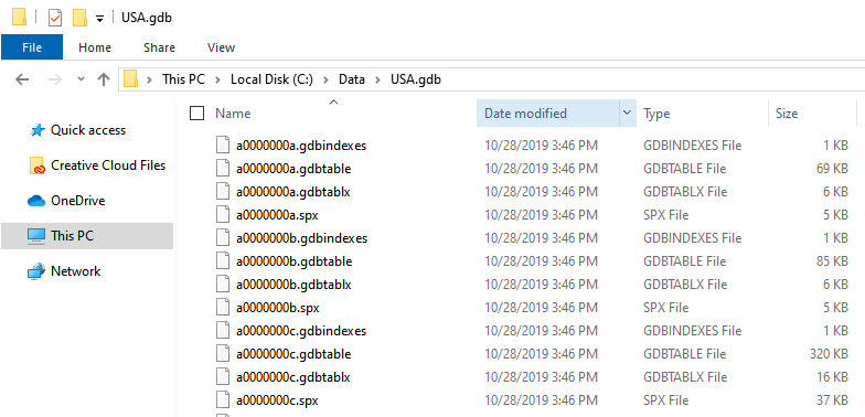
The safest way to get the paths you need is to open Pro's Catalog View (which displays in the middle of the application window, unlike the Catalog Pane, which displays on the right side of the application window) and browse to the dataset. The location box along the top indicates the folder or geodatabase whose contents are being viewed. Clicking on the dropdown arrow within that box displays the location as a network path. That's the path you want. Here's what the same file geodatabase would look like in Pro's Catalog view. The circled path shows how you would refer to a feature class's geodatabase then add the feature class name. (Alternatively, you could right-click any feature class from either the Catalog View or Catalog Pane, go to Properties, then click the Source tab to access its path.)
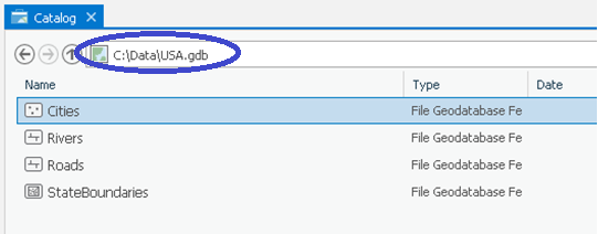
Below is an example of how you could access the feature class in a Python script using this path. This is similar to one of the examples in Lesson 1.
import arcpy
featureClass = "C:\\Data\\USA\\USA.gdb\\Cities"
desc = arcpy.Describe(featureClass)
spatialRef = desc.SpatialReference
print (spatialRef.Name)
Remember that the backslash (\) is a reserved character in Python, so you'll need to use either the double backslash (\\) or forward slash (/) in the path. Another technique you can use for paths is the raw string, which allows you to put backslashes and other reserved characters in your string as long as you put "r" before your quotation marks.
featureClass = r"C:\Data\USA\USA.gdb\Cities"
. . .
Workspaces
The Esri geoprocessing framework often uses the notion of a workspace to denote the folder or geodatabase where you're currently working. When you specify a workspace in your script, you don't have to list the full path to every dataset. When you run a tool, the geoprocessor sees the feature class name and assumes that it resides in the workspace you specified.
Workspaces are especially useful for batch processing, when you perform the same action on many datasets in the workspace. For example, you may want to clip all the feature classes in a folder to the boundary of your county. The workflow for this is:
- Define a workspace.
- Create a list of feature classes in the workspace.
- Define a clip feature.
- Configure a loop to run on each feature class in the list.
- Inside the loop, run the Clip tool.
Here's some code that clips each feature class in a file geodatabase to the Alabama state boundary, then places the output in a different file geodatabase. Note how the five lines of code after import arcpy correspond to the five steps listed above.
import arcpy

arcpy.env.workspace = "C:\\Data\\USA\\USA.gdb"
featureClassList = arcpy.ListFeatureClasses()
clipFeature = "C:\\Data\\Alabama\\Alabama.gdb\\StateBoundary"

for featureClass in featureClassList:
    arcpy.Clip_analysis(featureClass, clipFeature, "C:\\Data\\Alabama\\Alabama.gdb\\" + featureClass)
In the above example, the method arcpy.ListFeatureClasses() was the key to making the list. This method looks through a workspace and makes a Python list of each feature class in that workspace. Once you have this list, you can easily configure a for loop to act on each item.
Notice that you designated the path to the workspace using the location of the file geodatabase "C:\\Data\\USA\\USA.gdb". If you were working with shapefiles, you would just use the path to the containing folder as the workspace. You can download the USA.gdb here [3] and the Alabama.gdb here [4].
If you were working with ArcSDE, you would use the path to the .sde connection file when creating your workspace. This is a file that is created when you connect to ArcSDE in Catalog View, and is placed in your local profile directory. We won't be accessing ArcSDE data in this course, but if you do this at work, remember that you can use the location box as outlined above to help you understand the paths to datasets in ArcSDE.
3.2 Reading vector attribute data
Now that you know how to open a dataset, let's go a little bit deeper and start examining some individual data records. This section of the lesson discusses how to read and search data tables. These tables often provide the attributes for vector features, but they can also stand alone in some cases. The next section will cover how to write data to tables. At the end of the lesson, we'll look at rasters.
As we work with the data, it will be helpful for you to follow along, copying and pasting the example code into practice scripts. Throughout the lesson, you'll encounter exercises that you can do to practice what you just learned. You're not required to turn in these exercises; but if you complete them, you will have a greater familiarity with the code that will be helpful when you begin working on this lesson's project. It's impossible to read a book or a lesson, then sit down and write perfect code. Much of what you learn comes through trial and error and learning from mistakes. Thus, it's wise to write code often as you complete the lesson.
3.2.1 Accessing data fields
Before we get too deep into vector data access, it's going to be helpful to quickly review how the vector data is stored in the software. Vector features in ArcGIS feature classes (remember, including shapefiles) are stored in a table. The table has rows (records) and columns (fields).
Fields in the table
Fields in the table store the geometry and attribute information for the features.
There are two fields in the table that you cannot delete. One of the fields (usually called Shape) contains the geometry information for the features. This includes the coordinates of each vertex in the feature and allows the feature to be drawn on the screen. The geometry is stored in binary format; if you were to see it printed on the screen, it wouldn't make any sense to you. However, you can read and work with geometries using objects that are provided with arcpy.
The other field included in every feature class is an object ID field (OBJECTID or FID). This contains a unique number, or identifier for each record that is used by ArcGIS to keep track of features. The object ID helps avoid confusion when working with data. Sometimes records have the same attributes. For example, both Los Angeles and San Francisco could have a STATE attribute of 'California,' or a USA cities dataset could contain multiple cities with the NAME attribute of 'Portland;' however, the OBJECTID field can never have the same value for two records.
The rest of the fields contain attribute information that describe the feature. These attributes are usually stored as numbers or text.
Discovering field names
When you write a script, you'll need to provide the names of the particular fields you want to read and write. You can get a Python list of field names using arcpy.ListFields().
# Reads the fields in a feature class

import arcpy

featureClass = "C:\\Data\\USA\\USA.gdb\\Cities"
fieldList = arcpy.ListFields(featureClass)
# Loop through each field in the list and print the name
for field in fieldList:
    print (field.name)
The above would yield a list of the fields in the Cities feature class in a file geodatabase named USA.gdb. If you ran this script in PyScripter (try it with one of your own feature classes!) you would see something like the following in the IPython Console.
OBJECTID
Shape
UIDENT
POPCLASS
NAME
CAPITAL
STATEABB
COUNTRY
Notice the two special fields we already talked about: OBJECTID, which holds the unique identifying number for each record, and Shape, which holds the geometry for the record. Additionally, this feature class has fields that hold the name (NAME), the state (STATEABB), whether or not the city is a capital (CAPITAL), and so on.
arcpy treats the field as an object. Therefore the field has properties that describe it. That's why you can print field.name. The help reference topic Using fields and indexes [5] lists all the properties that you can read from a field. These include aliasName, length, type, scale, precision, and others.
Properties of a field are read-only, meaning that you can find out what the field properties are, but you cannot change those properties in a script using the Field object. If you wanted to change the scale and precision of a field, for instance, you would have to programmatically add a new field.
3.2.2 Reading through records
Now that you know how to traverse the table horizontally, reading the fields that are available, let's examine how to read up and down through the table records.
The arcpy module contains some objects called cursors that allow you to move through records in a table. There have been quite a few changes made to how cursors can be used over the different versions of ArcGIS, though the current best practice has been in place since version 10.1 of ArcGIS Desktop (aka ArcMap) and has carried over to ArcGIS Pro. If you find yourself working with code that was written for a pre-10.1 version of ArcMap, we suggest you check out this same page in our old ArcMap version of this course (see the content navigation links on the right side of the Drupal site). We will focus our discussion below on the current best practice in cursor usage, which you should be utilizing for scripts written in this course and in your workplace.
The arcpy data access module
At version 10.1 of ArcMap, Esri released a new data access module, which offered faster performance along with more robust behavior when crashes or errors were encountered with the cursor. The module contains different cursor classes for the different operations a developer might want to perform on table records -- one for selecting, or reading, existing records; one for making changes to existing records; and one for adding new records. We'll discuss the editing cursors later, focusing our discussion now on the cursor used for reading tabular data, the search cursor.
As with all geoprocessing classes, the SearchCursor class is documented in the Help system [6]. (Be sure when searching the Help system that you choose the SearchCursor class found in the Data Access module. An older, pre-10.1 class is available through the arcpy module and appears in the Help system as an "ArcPy Function.")
The common workflow for reading data with a search cursor is as follows:
- Create the search cursor. This is done through the method arcpy.da.SearchCursor(). This method takes several parameters in which you specify which dataset and, optionally, which specific rows you want to read.
- Set up a loop that will iterate through the rows until there are no more available to read.
- Within the loop, do something with the values in the current row.
Here's a very simple example of a search cursor that reads through a point dataset of cities and prints the name of each.
# Prints the name of each city in a feature class

import arcpy

featureClass = "C:\\Data\\USA\\USA.gdb\\Cities"

with arcpy.da.SearchCursor(featureClass,("NAME")) as cursor:
    for row in cursor:
        print (row[0])
Important points to note in this example:
- The cursor is created using a "with" statement. Although the explanation of "with" is somewhat technical, the key thing to understand is that it allows your cursor to exit the dataset gracefully, whether it crashes or completes its work successfully. This is a big issue with cursors, which can sometimes maintain locks on data if they are not exited properly.
- The "with" statement requires that you indent all the code beneath it. After you create the cursor in your "with" statement, you'll initiate a for loop to run through all the rows in the table. This requires additional indentation.
- Creating a SearchCursor object requires specifying not just the desired table/feature class, but also the desired fields within it, as a tuple. Remember that a tuple is a Python data structure much like a list, except it is enclosed in parentheses and its contents cannot be modified. Supplying this tuple speeds up the work of the cursor because it does not have to deal with the potentially dozens of fields included in your dataset. In the example above, the tuple contains just one field, "NAME".
- The "with" statement creates a SearchCursor object, and declares that it will be named "cursor" in any subsequent code.
- A for loop is used to iterate through the SearchCursor (using the "cursor" name assigned to it). Just as in a loop through a list, the iterator variable can be assigned a name of your choice (here, it's called "row").
- Retrieving values out of the rows is done using the index position of the field name in the tuple you submitted when you created the object. Since the above example submits only one item in the tuple, then the index position of "NAME" within that tuple is 0 (remember that we start counting from 0 in Python).
Here's another example where something more complex is done with the row values. This script finds the average population for counties in a dataset. To find the average, you need to divide the total population by the number of counties. The code below loops through each record and keeps a running total of the population and the number of records counted. Once all the records have been read, only one line of division is necessary to find the average. You can get the sample data for this script here. [7]
# Finds the average population in a counties dataset
import arcpy

featureClass = "C:\\Data\\Pennsylvania\\Counties.shp"
populationField = "POP1990"
nameField = "NAME"

average = 0
totalPopulation = 0
recordsCounted = 0

print("County populations:")

with arcpy.da.SearchCursor(featureClass, (nameField, populationField)) as countiesCursor:
    for row in countiesCursor:
        print (row[0] + ": " + str(row[1]))
        totalPopulation += row[1]

        recordsCounted += 1

average = totalPopulation / recordsCounted

print ("Average population for a county is " + str(average))
Differences between this example and the previous one:
- The tuple includes multiple fields, with their names having been stored in variables near the top of the script.
- The SearchCursor object goes by the variable name countiesCursor rather than cursor.
Before moving on, you should note that cursor objects have a couple of methods that you may find helpful in traversing their associated records. To understand what these methods do, and to better understand cursors in general, it may help to visualize the attribute table with an arrow pointing at the "current row." When a cursor is first created, that arrow is pointing just above the first row in the table. When a cursor is included in a for loop, as in the above examples, each execution of the for statement moves the arrow down one row and assigns that row's values (a tuple) to the row variable. If the for statement is executed when the arrow is pointing at the last row, there is not another row to advance to and the loop will terminate. (The row variable will be left holding the last row's values.)
Imagine that you wanted to iterate through the rows of the cursor a second time. If you were to modify the Cities example above, adding a second loop immediately after the first, you'd see that the second loop would never "get off the ground" because the cursor's internal pointer is still left pointing at the last row. To deal with this problem, you could just re-create the cursor object. However, a simpler solution would be to call on the cursor's reset() method. For example:
cursor.reset()
This will cause the internal pointer (the arrow) to move just above the first row again, enabling you to loop through its rows again.
The other method supported by cursor objects is the next() method, which allows you to retrieve rows without using a for loop. Returning to the internal pointer concept, a call to the next() method moves the pointer down one row and returns the row's values (again, as a tuple). For example:
row = cursor.next()
An alternative means of iterating through all rows in a cursor is to use the next() method together with a while loop. Here is the original Cities example modified to iterate using next() and while:
# Prints the name of each city in a feature class (using next() and while)

import arcpy

featureClass = "C:\\Data\\USA\\USA.gdb\\Cities"

with arcpy.da.SearchCursor(featureClass,("NAME")) as cursor:
    try:
        row = cursor.next()
        while row:
            print (row[0])
            row = cursor.next()
    except StopIteration:
        pass
Points to note in this script:
- This approach requires invoking next() both prior to the loop and within the loop.
- Calling the next() method when the internal pointer is pointing at the last row will raise a StopIteration exception. The example prevents that exception from displaying an ugly error.
You should find that using a for loop is usually the better approach, and in fact, you won't see the next() method even listed in the documentation of arcpy.da.SearchCursor. We're pointing out the existence of this method because a) older ArcGIS versions have cursors that can/must be traversed in this way, so you may encounter this coding pattern if looking at older scripts, and b) you may want to use the next() method if you're in a situation where you know the cursor will contain exactly one row (or you're interested in only the first row).
In each of the cursor examples discussed thus far, the cursors retrieved all rows from the specified feature class. Continue reading to see how to retrieve just a subset of rows meeting certain criteria.
3.2.3 Retrieving records using an attribute query
(Note: In this section, we are only using short code sections to read through, rather than full code examples that can be run directly. However, as an exercise, you can adapt the code to, for instance, work with the Pennsylvania data set from the previous section by using Counties.shp and the POP1990 field.)
The previous examples used the SearchCursor object to read through each record in a dataset. You can get more specific with the search cursor by instructing it to retrieve just the subset of records whose attributes comply with some criteria, for example, "only records with a population greater than 10000" or "all records beginning with the letters P – Z."
For review, this is how you construct a search cursor to operate on every record in a dataset using the arcpy.da module:
with arcpy.da.SearchCursor(featureClass,(populationField)) as cursor:
If you want the search cursor to retrieve only a subset of the records based on some criteria, you can supply a SQL expression (a where clause) as the third argument in the constructor (the constructor is the method that creates the SearchCursor). For example:
with arcpy.da.SearchCursor(featureClass, (populationField), "POP2018 > 100000") as cursor:
The above example uses the SQL expression POP2018 > 100000 to retrieve only the records whose population is greater than 100000. SQL stands for "Structured Query Language" and is a special syntax used for querying datasets. If you've ever used a Definition Query to filter a layer's data in Pro, then you've had some exposure to these sorts of SQL queries. If SQL is new to you, please take a few minutes right now to read Write a query in the Query Builder [8] in the ArcGIS Pro Help. This topic is a simple introduction to SQL in the context of ArcGIS.
SQL expressions can contain a combination of criteria, allowing you to pinpoint a very focused subset of records. The complexity of your query is limited only by your available data. For example, you could use a SQL expression to find only states with a population density over 100 people per square mile that begin with the letter M and were settled after 1850.
Note that the SQL expression you supply for a search cursor is for attribute queries, not spatial queries. You could not use a SQL expression to select records that fall "west of the Mississippi River," or "inside the boundary of Canada" unless you had previously added and populated some attribute stating whether that condition were true (for example, REGION = 'Western' or CANADIAN = True). Later in this lesson, we'll talk about how to make spatial queries using the Select By Location geoprocessing tool.
Once you retrieve the subset of records, you can follow the same pattern of iterating through them using a for loop.
with arcpy.da.SearchCursor(featureClass, (populationField), "POP2018 > 100000") as cursor:
    for row in cursor:
        print (str(row[0]))
Handling quotation marks
When you include a SQL expression in your SearchCursor constructor, you must supply it as a string. This is where things can get tricky with quotation marks since parts of the expression may also need to be quoted (specifically string values, such as a state abbreviation). The rule for writing queries in ArcGIS Pro is that string values must be enclosed in single quotes. Given that, you should enclose the overall expression in double quotes.
For example, suppose your script allows the user to enter the ID of a parcel, and you need to find it with a search cursor. Your SQL expression might look like this: " PARCEL = 'A2003KSW' ".
Handling quotation marks is simplified greatly in Pro as compared to ArcMap. In ArcMap, certain data formats require field names to be enclosed in double quotes, which when combined with string values being present in the expression, can make constructing the expression correctly quite a headache. If you find yourself needing to write ArcMap scripts that query data, check out the parallel page in the ArcMap version of this lesson (see course navigation links to the right).
Selecting records by attribute
As an ArcGIS Pro user, you've probably clicked the Select By Attributes button, located under the Map tab, to perform attribute queries. What we've been talking about in this part of the lesson probably reminded you of doing that sort of query, but it's important to note that opening a search cursor with a SQL expression (or where clause) as described above is not quite the same sort of operation. A search cursor is used in situations where you want to do some sort of processing of the records one by one. For example, as we saw, printing the names of cities or calculating their average population.
Some situations instead call for creating a selection on the feature class (i.e., treating the features identified by the query as a single unit). This can be done in Python scripts by invoking the Select Layer By Attribute tool (which is actually the tool that opens when you click the Select By Attributes button in Pro). The output from this tool -- referred to as a Feature Layer -- can then be used as the input to many other tools (Calculate Field, Copy Features, Delete Features, to name a few). This second tool's processing will be limited to the selection held in the input.
For an example, let's pick up on the population query used above. Let's say we wanted to do an analysis in which high-population cities were excluded. We might select those cities and then delete them:
popQuery = 'POP2018 > 100000'
bigCities = arcpy.SelectLayerByAttribute_management('Cities', 'NEW_SELECTION', popQuery)
arcpy.DeleteFeatures_management(bigCities)
In this snippet of code, note that the same where clause is implemented, this time to create a selection on the Cities feature class as opposed to producing a cursor of records to iterate through. The SelectLayerByAttribute tool returns a Feature Layer, which is an in-memory object that references the selected features. The object is stored in a variable, bigCities, which is then used as input to the DeleteFeatures tool. This will delete the high-population cities from the underlying Cities feature class.
Now, let's have a look at how to handle queries with spatial constraints.
3.2.4 Retrieving records using a spatial query
Applying a SQL expression to the search cursor is only useful for attribute queries, not spatial queries. For example, you can easily open a search cursor on all counties named "Lincoln" using a SQL expression, but finding all counties that touch or include the Mississippi River requires a different approach. To get a subset of records based on a spatial criterion, you need to use the geoprocessing tool Select Layer By Location.
Note:
A few relational databases such as SQL Server expose spatial data types that can be spatially queried with SQL. Support for these spatial types in ArcGIS is still maturing, and in this course, we will assume that the way to make a spatial query is through Select Layer By Location. Since we are not using ArcSDE, this is actually true.
Suppose you want to generate a list of all states whose boundaries touch Wyoming. As we saw in the previous section with the Select Layer By Attribute tool, the Select Layer By Location tool will return a Feature Layer containing the features that meet the query criteria. One thing we didn't mention in the previous section is that a search cursor can be opened not only on feature classes, but also on feature layers. With that in mind, here is a set of steps one might take to produce a list of Wyoming's neighbors:
- Use Select Layer By Attribute on the states feature class to create a feature layer of just Wyoming. Let's call this the Selection State layer.
- Use Select Layer By Location on the states feature class to create a feature layer of just those states that touch the Selection State layer. Let's call this the Neighbors layer.
- Open a search cursor on the Neighbors layer. The cursor will include only Wyoming and the states that touch it because the Neighbors layer is the selection applied in step 2 above. Remember that the feature layer is just a set of records held in memory.
Below is some code that applies the above steps.
# Selects all states whose boundaries touch
# a user-supplied state
import arcpy

# Get the US States layer, state, and state name field
usaFC = r"C:\Data\USA\USA.gdb\Boundaries"
state = "Wyoming"
nameField = "NAME"

try:
    whereClause = nameField + " =  '" + state + "'"
    selectionStateLayer = arcpy.SelectLayerByAttribute_management(usaFC, 'NEW_SELECTION', whereClause)

    # Apply a selection to the US States layer
    neighborsLayer = arcpy.SelectLayerByLocation_management(usaFC, 'BOUNDARY_TOUCHES', selectionStateLayer)

    # Open a search cursor on the US States layer
    with arcpy.da.SearchCursor(neighborsLayer, (nameField)) as cursor:
        for row in cursor:
            # Print the name of all the states in the selection
            print (row[0])

except:
    print (arcpy.GetMessages())

finally:
    # Clean up feature layers and cursor
    arcpy.Delete_management(neighborsLayer)
    arcpy.Delete_management(selectionStateLayer)
    del cursor
You can choose from many spatial operators when running SelectLayerByLocation. The code above uses "BOUNDARY_TOUCHES". Other available relationships are "INTERSECT", "WITHIN A DISTANCE" (may save you a buffering step), "CONTAINS", "CONTAINED_BY", and others.
Note that the Row object "row" returns only one field ("NAME"), which is accessed using its index position in the list of fields. Since there's only one field, that index is 0, and the syntax looks like this: row[0]. Once you open the search cursor on your selected records, you can perform whatever action you want on them. The code above just prints the state name, but more likely you'll want to summarize or update attribute values. You'll learn how to write attribute values later in this lesson.
Cleaning up feature layers and cursors
Notice that the feature layers are deleted using the Delete tool. This is because feature layers can maintain locks on your data, preventing other applications from using the data until your script is done. arcpy is supposed to clean up feature layers at the end of the script, but it's a good idea to delete them yourself in case this doesn't happen or in case there is a crash. In the examples above, the except block will catch a crash, then the script will continue and Delete the two feature layers.
Cursors can also maintain locks on data. As mentioned earlier, the "with" statement should clean up the cursor for you automatically. However, we've found that it doesn't always, an observation that appears to be backed up by this blurb from Esri's documentation of the arcpy.da.SearchCursor class [6]:
Search cursors also support with statements to reset iteration and aid in removal of locks. However, using a del statement to delete the object or wrapping the cursor in a function to have the cursor object go out of scope should be considered to guard against all locking cases.
One last point to note about this code that cleans up the feature layers and cursor is that it is embedded within a finally block. This is a construct that is used occasionally with try and except to define code that should be executed regardless of whether the statements in the try block run successfully. To understand the usefulness of finally, imagine if you had instead placed these cleanup statements at the end of the try block. If an error were to occur somewhere above that point in the try block -- not hard to imagine, right? -- the remainder of the try block would not be executed, leaving the feature layers and cursor in memory. A subsequent run of the script, after fixing the error, would encounter a new problem: the script would be unable to create the feature layer stored in selectionStatesLayer because it already exists. In other words, the cleanup statements would only run if the rest of the script ran successfully.
This situation is where the finally statement is especially helpful. Code in a finally block will be run regardless of whether something in the try block triggers a crash. (In the event that an error is encountered, the finally code will be executed after the except code.) Thus, as you develop your own code utilizing feature layers and/or cursors, it's a good idea to include these cleanup statements in a finally block.
Alternate syntax
Implementation of the Select Layer By Attribute/Location tools required a different syntax in earlier versions of ArcGIS. The tools didn't return a Feature Layer, and instead they required you to first create the Feature Layer yourself using the Make Feature Layer tool. Let's have a look at this same example completed using that syntax:
# Selects all states whose boundaries touch
#  a user-supplied state

import arcpy

# Get the US States layer, state, and state name field
usaFC = r"C:\Data\USA\USA.gdb\Boundaries"
state = "Wyoming"
nameField = "NAME"

try:
    # Make a feature layer with all the US States
    arcpy.MakeFeatureLayer_management(usaFC, "AllStatesLayer")

    whereClause = nameField + " =  '" + state + "'"

    # Make a feature layer containing only the state of interest
    arcpy.MakeFeatureLayer_management(usaFC, "SelectionStateLayer", whereClause)

    # Apply a selection to the US States layer
    arcpy.SelectLayerByLocation_management("AllStatesLayer","BOUNDARY_TOUCHES","SelectionStateLayer")

    # Open a search cursor on the US States layer
    with arcpy.da.SearchCursor("AllStatesLayer", (nameField)) as cursor:
        for row in cursor:
            # Print the name of all the states in the selection
            print (row[0])

except:
    print (arcpy.GetMessages())

finally:
    # Clean up feature layers and cursor
    arcpy.Delete_management("AllStatesLayer")
    arcpy.Delete_management("SelectionStateLayer")
    del cursor
Note that the first MakeFeatureLayer statement takes the Boundaries feature class as an input and produces as an output a feature layer that throughout the rest of the script can be referred to using the name 'AllStatesLayer.' Similarly, the next statement creates another feature layer from the Boundaries feature class, this one applying a where clause to limit the included features to just Wyoming. This feature layer will go by the name 'SelectionStateLayer.' Creation of these feature layers was necessary in this older syntax because the Select Layer By Attribute/Location tools would only recognize feature layers, not feature classes, as valid inputs.
While we find this syntax to be a bit odd and less intuitive than the one shown at the beginning of this section, it still works, and you may encounter it when viewing others' scripts.
Required reading
Before you move on, examine the following tool reference pages. Pay particular attention to the Usage and the Code Sample sections.
3.3 Writing vector attribute data
In the same way that you use cursors to read vector attribute data, you use cursors to write data as well. Two types of cursors are supplied for writing data:
- Update cursor - This cursor edits values in existing records or deletes records
- Insert cursor - This cursor adds new records
In the following sections, you'll learn about both of these cursors and get some tips for using them.
Required reading
The ArcGIS Pro Help has some explanation of cursors. Get familiar with this help now, as it will prepare you for the next sections of the lesson. You'll also find it helpful to return to the code examples while working on Project 3:
Accessing data using cursors [12]
Also follow the three links in the table at the beginning of the above topic. These briefly explain the InsertCursor [13], SearchCursor [6], and UpdateCursor [14] and provide a code example for each. You've already worked with SearchCursor, but closely examine the code examples for all three cursor types and see if you can determine what is happening in each.
3.3.1 Updating existing records
Use the update cursor to modify existing records in a dataset. Here are the general steps for using the update cursor:
- Create the update cursor by calling arcpy.da.UpdateCursor(). You can optionally pass in an SQL expression as an argument to this method. This is a good way to narrow down the rows you want to edit if you are not interested in modifying every row in the table.
- Use a for loop to iterate through the rows and for each row...
- Modify the field values in the row that need updating (see below).
- Call UpdateCursor.updateRow() to finalize the edit.
Modifying field values
When you create an UpdateCursor and iterate through the rows using a variable called row, you can modify the field values by making assignments using the syntax row[<index of the field you want to change>] = <the new value>. For example:
row[0] = "Trisha Stevens"
It is important to note that the index occurring in the [...] to determine which field will be changed is given with respect to the tuple of fields provided when the UpdateCursor is created. For instance, if we create the cursor using the following command
with arcpy.da.UpdateCursor(featureClass, ("CompanyName", "Owner")) as cursor:
row[0] would refer to the field called "CompanyName" and row[1] refers to the field that has the name "Owner".
Example
The script below performs a "search and replace" operation on an attribute table. For example, suppose you have a dataset representing local businesses, including banks. One of the banks was recently bought out by another bank. You need to find every instance of the old bank name and replace it with the new name. This script could perform that task automatically.
#Simple search and replace script
import arcpy

# Retrieve input parameters: the feature class, the field affected by
#  the search and replace, the search term, and the replace term.
fc = arcpy.GetParameterAsText(0)
affectedField = arcpy.GetParameterAsText(1)
oldValue = arcpy.GetParameterAsText(2)
newValue = arcpy.GetParameterAsText(3)

# Create the SQL expression for the update cursor. Here this is
#  done on a separate line for readability.
queryString = affectedField + " = '" + oldValue + "'"

# Create the update cursor and update each row returned by the SQL expression
with arcpy.da.UpdateCursor(fc, (affectedField), queryString) as cursor:
    for row in cursor:
        row[0] = newValue
        cursor.updateRow(row)

del row, cursor
Notice that this script is relatively flexible because it gets all the parameters as text. However, this script can only be run on string variables because of the way the query string is set up. Notice that the old value is put in quotes, like this: "'" + oldValue + "'". Handling other types of variables, such as integers, would have made the example longer.
Again, it is critical to understand the tuple of affected fields that you pass in when you create the update cursor. In this example, there is only one affected field (which we named affectedField), so its index position is 0 in the tuple. Therefore, you set that field value using row[0] = newValue.
The last line with updateRow(...) is needed to make sure that the modified row is actually written back to the attribute table. Please note that the variable row needs to be passed as a parameter to updateRow(...).
Dataset locking again
As we mentioned, ArcGIS sometimes places locks on datasets to avoid the possibility of editing conflicts between two users. If you think for any reason that a lock from your script is affecting your dataset (by preventing you from viewing it, making it look like all rows have been deleted, and so on), you must close PyScripter to remove the lock. If you think that Pro has a lock on your data, check to see if there is an open edit session on the data, the data is being displayed in the Catalog View/Pane, or if a layer based on the data is part of an open map.
As we stated, cursor cleanup should happen through the creation of the cursor inside a "with" statement, but adding lines to delete the row and cursor objects will make extra sure locks are released.
For the Esri explanation of how locking works, you can review the section "Cursors and locking" in the topic Accessing data using cursors [15] in the ArcGIS Pro Help.
3.3.2 Inserting new records
When adding a new record to a table, you must use the insert cursor. Here's the workflow for insert cursors:
- Create the insert cursor using arcpy.da.InsertCursor().
- Call InsertCursor.insertRow() to add a new row to the dataset.
As with the search and update cursor, you can use an insert cursor together with the "with" statement to avoid locking problems.
Insert cursors differ from search and update cursors in that you cannot provide an SQL expression when you create the insert cursor. This makes sense because an insert cursor is only concerned with adding records to the table. It does not need to "know" about the existing records or any subset thereof.
When you insert a row using InsertCursor.insertRow(), you provide a comma-delimited tuple of values for the fields of the new row. The order of these values must match the order of values of the tuple of affected fields you provided when you created the cursor. For example, if you create the cursor using
with arcpy.da.InsertCursor(featureClass, ("FirstName","LastName")) as cursor:
you would add a new row with values "Sam" for "FirstName" and "Fisher" for "LastName" by the following command:
cursor.insertRow(("Sam","Fisher"))
Please note that the inner parentheses are needed to turn the values into a tuple that is passed to insertRow(). Writing cursor.insertRow("Sam","Fisher") would have resulted in an error.
Example
The example below uses an insert cursor to create one new point in the dataset and assign it one attribute: a string description. This script could potentially be used behind a public-facing 311 [16] application, in which members of the public can click a point on a Web map and type a description of an incident that needs to be resolved by the municipality, such as a broken streetlight.
# Adds a point and an accompanying description
import arcpy
# Retrieve input parameters
inX = arcpy.GetParameterAsText(0)
inY = arcpy.GetParameterAsText(1)
inDescription = arcpy.GetParameterAsText(2)

# These parameters are hard-coded. User can't change them.
incidentsFC = "C:/Data/Yakima/Incidents.shp"
descriptionField = "DESCR"

# Make a tuple of fields to update
fieldsToUpdate = ("SHAPE@XY", descriptionField)
# Create the insert cursor
with arcpy.da.InsertCursor(incidentsFC, fieldsToUpdate) as cursor:
    # Insert the row providing a tuple of affected attributes
    cursor.insertRow(((float(inX),float(inY)), inDescription))

del cursor
Take a moment to ensure that you know exactly how the following is done in the code:
- The creation of the insert cursor with a tuple of affected fields stored in variable fieldsToUpdate
- The insertion of the row through the insertRow() method using variables that contain the field values of the new row
If this script really were powering an interactive 311 application, the X and Y values could be derived from a point a user clicked on the Web map rather than as parameters as done in lines 4 and 5.
One thing you might have noticed is that the string "SHAPE@XY" is used to specify the Shape field. You might expect that this would just be "Shape," but arcpy.da provides a list of "tokens" that you can use if the field will be specified in a certain way. In our case, it would be very convenient just to provide the X and Y values of the points using a tuple of coordinates. It turns out that the token "SHAPE@XY" allows you to do just that. See the documentation of the InsertCursor's field_names parameter [13] to learn about other tokens you can use.
Putting this all together, the example creates a tuple of affected fields: ("SHAPE@XY", "DESCR"). Notice that in line 13, we actually use the variable descriptionField which contains the name of the second column "DESCR" for the second element of the tuple. Using a variable to store the name of the column we are interested in allows us to easily adapt the script later, for instance to a data set where the column has a different name. When the row is inserted, the values for these items are provided in the same order: cursor.insertRow(((float(inX), float(inY)), inDescription)). The argument passed to insertRow() is a tuple that contains another tuple (inX,inY), namely the coordinates of the point cast to floating point numbers, as the first element and the text for the "DESCR" field as the second element.
Readings
Take a few minutes to read Zandbergen 8.1 - 8.3 to reinforce your learning about cursors.
3.4 Working with rasters
So far in this lesson, your scripts have only read and edited vector datasets. This work largely consists of cycling through tables of records and reading and writing values to certain fields. Raster data is very different, and consists only of a series of cells, each with its own value. So, how do you access and manipulate raster data using Python?
It's unlikely that you will ever need to cycle through a raster cell by cell on your own using Python, and that technique is outside the scope of this course. Instead, you'll most often use predefined tools to read and manipulate rasters. These tools have been designed to operate on various types of rasters and perform the cell-by-cell computations so that you don't have to.
In ArcGIS, most of the tools you'll use when working with rasters are in either the Data Management > Raster toolset or the Spatial Analyst toolbox. These tools can reproject, clip, mosaic, and reclassify rasters. They can calculate slope, hillshade, and aspect rasters from DEMs.
The Spatial Analyst toolbox also contains tools for performing map algebra on rasters. Multiplying or adding many rasters together using map algebra is important for GIS site selection scenarios. For example, you may be trying to find the best location for a new restaurant and you have seven criteria that must be met. If you can create a boolean raster (containing 1 for suitable, 0 for unsuitable) for each criterion, you can use map algebra to multiply the rasters and determine which cells receive a score of 1, meeting all the criteria. (Alternatively, you could add the rasters together and determine which areas received a value of 7.) Other courses in the Penn State GIS certificate program walk through these types of scenarios in more detail.
The tricky part of map algebra is constructing the expression, which is a string stating what the map algebra operation is supposed to do. ArcGIS Pro contains interfaces for constructing an expression for one-time runs of the tool. But what if you want to run the analysis several times, or with different datasets? It's challenging even in ModelBuilder to build a flexible expression into the map algebra tools. With Python, you can manipulate the expression as much as you need.
Example
Examine the following example, which takes in a minimum and maximum elevation value as parameters, then does some map algebra with those values. The expression isolates areas where the elevation is greater than the minimum parameter and less than the maximum parameter. Cells that satisfy the expression are given a value of 1 by the software, and cells that do not satisfy the expression are given a value of 0.
But what if you don't want those 0 values cluttering your raster? This script gets rid of the 0's by running the Reclassify tool with a real simple remap table stating that input raster values of 1 should remain 1. Because 0 is left out of the remap table, it gets reclassified as NoData:
# This script takes a DEM, a minimum elevation,
#  and a maximum elevation. It outputs a new
#  raster showing only areas that fall between
#  the min and the max

import arcpy
from arcpy.sa import *
arcpy.env.overwriteOutput = True
arcpy.env.workspace = "C:/Data/Elevation"

# Get parameters of min and max elevations
inMin = arcpy.GetParameterAsText(0)
inMax = arcpy.GetParameterAsText(1)

arcpy.CheckOutExtension("Spatial")

# Perform the map algebra and make a temporary raster
inDem = Raster("foxlake")
tempRaster = (inDem > int(inMin)) & (inDem < int(inMax))

# Set up remap table and call Reclassify, leaving all values not 1 as NODATA
remap = RemapValue([[1,1]])
remappedRaster = Reclassify(tempRaster, "Value", remap, "NODATA")

# Save the reclassified raster to disk
remappedRaster.save("foxlake_recl")

arcpy.CheckInExtension("Spatial")
Read the example above carefully, as many times as necessary, for you to understand what is occurring in each line. Notice the following things:
- Notice the expression contains > and < signs, as well as the & operator. You have to enclose each side of the expression in parentheses to avoid confusing the & operator.
- Because you used arcpy.GetParameterAsText() to get the input parameters, you have to cast the input to an integer before you can do map algebra with it. If we just used inMin, the software would see "3000," for example, and would try to interpret that as a string. To do the numerical comparison, we have to use int(inMin). Then the software sees the number 3000 instead of the string "3000."
- Map algebra can perform many types of math and operations on rasters, not limited to "greater than" or "less than." For example, you can use map algebra to find the cosine of a raster.
- If you're working at a site where a license manager restricts the Spatial Analyst extension to a certain number of users, you must check out the extension in your script, then check it back in. Notice the calls to arcpy.CheckOutExtension() and arcpy.CheckInExtension(). You can pass in other extensions besides "Spatial" as arguments to these methods.
- Notice that the script doesn't call these Spatial Analyst functions using arcpy. Instead, it imports functions from the Spatial Analyst module (from arcpy.sa import *) and calls the functions directly. For example, we don't see arcpy.Reclassify(); instead, we just call Reclassify() directly. This can be confusing for beginners (and old pros) so be sure to check the Esri samples closely for each tool you plan to run. Follow the syntax in the samples and you'll usually be safe.
- See the Remap classes [17] topic in the help to understand how the remap table in this example was created. Whenever you run Reclassify, you have to create a remap table stating how the old values should be reclassified to new values. This example has about the simplest remap table possible, but if you want a more complex remap table, you'll need to study the documentation.
Rasters and file extensions
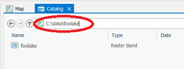
The above example script doesn't use any file extensions for the rasters. This is because the rasters use the Esri GRID format, which doesn't use extensions. If you have rasters in another format, such as .jpg, you will need to add the correct file extension. If you're unsure of the syntax to use when providing a raster file name, double click the raster in Catalog View and note its Location in the pop-out box.
If you look at rasters such as an Esri GRID in Windows Explorer, you may see that they actually consist of several supporting files with different extensions, sometimes even contained in a series of folders. Don't try to guess one of the files to reference; instead, use Catalog View to get the path to the raster. When you use this path, the supporting files and folders will work together automatically.
Readings
Zandbergen chapter 10 covers a lot of additional functions you can perform with rasters and has some good code examples. You don't have to understand everything in this chapter, but it might give you some good ideas for your final project.
Lesson 3 Practice Exercises
Lessons 3 and 4 contain practice exercises that are longer than the previous practice exercises and are designed to prepare you specifically for the projects. You should make your best attempt at each practice exercise before looking at the solution. If you get stuck, study the solution until you understand it.
Don't spend so much time on the practice exercises that you neglect Project 3. However, successfully completing the practice exercises will make Project 3 much easier and quicker for you.
Data for Lesson 3 practice exercises
The data for the Lesson 3 practice exercises is very simple and, like some of the Project 2 practice exercise data, was derived from Washington State Department of Transportation [18] datasets. Download the data here [19].
Using the discussion forums
Using the discussion forums is a great way to work towards figuring out the practice exercises. You are welcome to post blocks of code on the forums relating to these exercises.
When completing the actual Project 3, avoid posting blocks of code longer than a few lines. If you have a question about your Project 3 code, please email the instructor, or you can post general questions to the forums that don't contain more than a few lines of code.
Getting ready
If the practice exercises look daunting to you, you might start by practicing with your cursors a little bit using the sample data:
- Try to loop through the CityBoundaries and print the name of each city.
- Try using an SQL expression with a search cursor to print the OBJECTIDs of all the park and rides in Chelan county (notice there is a County field that you could put in your SQL expression).
- Use an update cursor to find the park and ride with OBJECTID 336. Assign it a ZIP code of 98512.
You can post thoughts on the above challenges on the forums.
Lesson 3 Practice Exercise A
In this practice exercise, you will programmatically select features by location and update a field for the selected features. You'll also use your selection to perform a calculation.
In your Lesson3PracticeExerciseA folder, you have a Washington geodatabase with two feature classes:
- CityBoundaries - Contains polygon boundaries of cities in Washington over 10 square kilometers in size.
- ParkAndRide - Contains point features representing park and ride facilities where commuters can leave their cars.
The objective
You want to find out which cities contain park and ride facilities and what percentage of cities have at least one facility.
- The CityBoundaries feature class has a field "HasParkAndRide," which is set to "False" by default. Your job is to mark this field "True" for every city containing at least one park and ride facility within its boundaries.
- Your script should also calculate the percentage of cities that have a park and ride facility and print this figure for the user.
You do not have to make a script tool for this assignment. You can hard-code the variable values. Try to group the hard-coded string variables at the beginning of the script.
For the purposes of these practice exercises, assume that each point in the ParkAndRide dataset represents one valid park and ride (ignore the value in the TYPE field).
Tips
You can jump into the assignment at this point, or read the following tips to give you some guidance.
- Make two feature layers: "CitiesLayer" and "ParkAndRideLayer."
- Use SelectLayerByLocation with a relationship type of "CONTAINS" to narrow down your cities feature layer list to only the cities that contain park and rides.
- Create an update cursor for your now narrowed-down "CitiesLayer" and loop through each record, setting the HasParkAndRide field to "True."
- To calculate the percentage of cities with park and rides, you'll need to know the total number of cities. You can use the GetCount [20] tool to get a total without writing a loop. Beware that this tool has an unintuitive return value that isn't well documented. The return value is a Result object, and the count value itself can be retrieved through that object by appending [0] (see the second code example from the Help). This will return the count as a string though, so you'll want to cast to an integer before trying to use it in an arithmetic expression.
- Similarly, you may have to play around with your Python math a little to get a nice percentage figure. Don't get too hung up on this part.
Lesson 3 Practice Exercise A Solution
Below is one possible solution to Practice Exercise A with comments to explain what is going on. If you find a more efficient way to code a solution, please share it through the discussion forums. Please note that in order to make the changes to citiesLayer permanent, you have to write the layer back to disk using the arcpy.CopyFeatures_management(...) function. This is not shown in the solution here.
# This script determines the percentage of cities in the
#  state with park and ride facilities

import arcpy

arcpy.env.overwriteOutput = True
arcpy.env.workspace = r"C:\PSU\geog485\L3\PracticeExerciseA\Washington.gdb"
cityBoundariesFC = "CityBoundaries"
parkAndRideFC = "ParkAndRide"
parkAndRideField = "HasParkAndRide"   # Name of column with Park & Ride information
citiesWithParkAndRide = 0             # Used for counting cities with Park & Ride

try:
    # Narrow down the cities layer to only the cities that contain a park and ride
    citiesLayer = arcpy.SelectLayerByLocation_management(cityBoundariesFC, "CONTAINS", parkAndRideFC)

    # Create an update cursor and loop through the selected records
    with arcpy.da.UpdateCursor(citiesLayer, (parkAndRideField)) as cursor:
        for row in cursor:
            # Set the park and ride field to TRUE and keep a tally
            row[0] = "True"
            cursor.updateRow(row)
            citiesWithParkAndRide += 1
except:
    print ("There was a problem performing the spatial selection or updating the cities feature class")

# Delete the feature layers even if there is an exception (error) raised
finally:
    arcpy.Delete_management(citiesLayer)
    del row, cursor

# Count the total number of cities (this tool saves you a loop)
numCitiesCount = arcpy.GetCount_management(cityBoundariesFC)
numCities = int(numCitiesCount[0])

# Get the number of cities in the feature layer
#citiesWithParkAndRide = int(citiesLayer[2])

# Calculate the percentage and print it for the user
percentCitiesWithParkAndRide = (citiesWithParkAndRide / numCities) * 100

print (str(round(percentCitiesWithParkAndRide,1)) + " percent of cities have a park and ride.")
Below is a video offering some line-by-line commentary on the structure of this solution:
Video: One Solution to Lesson 3, Practice Exercise A (9:37)
This video shows one solution to Lesson 3, Practice Exercise A, which determines the percentage of cities in the State of Washington that have park and ride facilities.
This solution uses the syntax currently shown in the ArcGIS Pro documentation for Select Layer By Location, in which the FeatureLayer returned by the tool is stored in a variable.
Looking at this solution, I start by importing the arcpy site package. Then I added this line 6 to set the overwriteOutput property to True, which is useful when you're writing scripts like these where you'll be doing some testing, and you'll often want to overwrite the output files. Otherwise, ArcGIS will return an error message saying that it cannot overwrite an output that already exists. So, that's a tip to take from this code.
On line 7, I set the workspace to the Washington file geodatabase that stores the data used in the exercise. That enables me to refer to the input feature classes using only their names, not their full paths. This script doesn’t produce any new output feature classes, but if it did, I could likewise specify them using only their names and not their full paths.
So, in lines 8 & 9, I define variables to refer to the CityBoundaries and ParkAndRide feature classes.
The purpose of this script is to update a field in the CityBoundaries feature class called HasParkAndRide with either a True or False value. So on line 10 I define a parkAndRideField variable to store the name of that field I’m going to be updating.
I also want to report the percentage of cities containing a park and ride at the end of the script through a print statement, so on line 11 I define a variable to store a count of those cities and I initialize that variable to 0.
Now, before I talk about the meat of the script, it’s often helpful to walk through your processing steps manually in Pro. So here I have the ParkAndRides, symbolized by black dots, and the city boundaries that are the orange polygons.
So, I can use the Select By Location tool and specify that I want to select the CityBoundaries features that contain ParkAndRide features. You can see all the city features selected, and I can open the attribute table to see the selected tabular records. I've got 74 of 108 selected. And then over here is the HasParkAndRide field that I would want to update to True for these selected records.
Getting back to my script, I’m going to implement the same Select By Location tool. It’s going to return to me a Feature Layer of cities that contain a ParkAndRide, which I store in my citiesLayer variable. I then open up an update cursor on that Feature Layer. This update cursor will only be able to update the fields that I specify in the second parameter. I could include any number of fields here, as a tuple, but for this scenario I really only need to include one. And the name of that field is stored in my parkAndRideField variable, which I had defined up on line 10.
And so what I have is a cursor that I can iterate through row by row. And I do that using a for loop, which starts on line 19. And on line 21, I take that HasParkAndRide field, and I set it to “True”.
Now, why do I say 0 there in square brackets? 0 is the index position of the field that I passed in that tuple in line 18. The first, and in this case the only, field in the tuple is at position 0.
If I was updating three or four fields, I would have row and then the field index position inside brackets. It could be 1, 2, 3, and so on.
After I've made my changes, I need to call updateRow() in order for them to be applied. A mistake that a lot of beginners make is they forget to do this step. So in line 22, I'm calling updateRow().
And in line 23, I'm incrementing the counter that I'm keeping of the number of cities with a park and ride facility found. So I just add 1 to the counter. The plus-equals-1 syntax is a shortcut for saying take the number in this variable and add 1.
I'm using try/except here to provide a custom error message. An important part of this script that goes along with this try/except block is this finally block on lines 28-30. This contains code that I want to run whether or not the try code failed. I don’t want to leave a lock in place on the cities feature class, so I delete the Feature Layer based on it on line 29. I also use a Python del statement to clear the row and cursor objects out of memory, for the same reason I used arcpy’s Delete tool: to make sure no locks are left on the feature classes.
Now, I could have put these statements in the try block, say after the update cursor, and assuming there were no problems in running my code, those clean-up statements would get executed too. However, let’s say there was a problem in my update cursor. If the script crashes there, then my clean-up statements won’t get executed, and if I try to run the script again, I could run into a problem with the cities feature class having a lock on it. Putting the clean-up statements in the finally block ensures they’ll get executed in all situations.
Now that I've done the important stuff, it's time to do some math to figure out the percentage of cities that have a park and ride facility. So in line 33, I'm running the GetCount tool in ArcGIS. When you use the GetCount tool, it’s a bit unintuitive because what it returns isn’t a number, but a result object. What you can do with that object isn’t well documented, so you can just follow on the example here and use [0] to get at the count in string form, and use the int() function to convert that string to an integer.
So what we have in the end, on line 34, is a variable called numCities that is the total number of cities in the entire data set. And then, we've already been keeping the counter of cities that have a park and ride. So to find the percentage, all we need to do is divide one by the other. And that's what's going on in line 40.
Now, you may have noticed line 37 refers to the citiesWithParkAndRide variable, but is commented out. It turns out that the object returned by SelectLayerByLocation (and SelectLayerByAttribute) isn’t just the Feature Layer of selected cities. Like the GetCount tool we just saw, the Select tools actually return a Result object. This object can be treated kind of like a list. If you want the Feature Layer, you can specify [0] or simply not include a number in brackets at all. But you can also get a count of the selected features by specifying [2]. You can see this in the documentation of the tool, in the Derived Output section.
So, it turns out we don’t really need to implement our own counter inside the loop through the cursor rows. We can get the count through the Result object, and thus we could uncomment line 37 and comment out lines 23 and 11. We decided to include the counter approach in this solution because as a programmer, there are bound to be times where you really do need to maintain your own counter, and we wanted you to see an example of how to do that.
Finally, we can print out the result at the end of the script in line 42. The percentage is a number with several digits after the decimal point, so the print statement first rounds the number to one digit after the decimal and then converts that value to a string so that it can be concatenated with the literal text.
Here is a different solution to Practice Exercise A, which uses the alternate syntax discussed in the lesson:
# This script determines the percentage of cities in the
#  state with park and ride facilities

import arcpy

arcpy.env.overwriteOutput = True
arcpy.env.workspace = r"C:\PSU\geog485\L3\PracticeExerciseA\Washington.gdb"
cityBoundariesFC = "CityBoundaries"
parkAndRideFC = "ParkAndRide"
parkAndRideField = "HasParkAndRide"   # Name of column with Park & Ride information
citiesWithParkAndRide = 0             # Used for counting cities with Park & Ride

try:
    # Make a feature layer of all the park and ride facilities
    arcpy.MakeFeatureLayer_management(parkAndRideFC, "ParkAndRideLayer")

    # Make a feature layer of all the cities polygons
    arcpy.MakeFeatureLayer_management(cityBoundariesFC, "CitiesLayer")

except:
    print ("Could not create feature layers")

try:
    # Narrow down the cities layer to only the cities that contain a park and ride
    arcpy.SelectLayerByLocation_management("CitiesLayer", "CONTAINS", "ParkAndRideLayer")

    # Create an update cursor and loop through the selected records
    with arcpy.da.UpdateCursor("CitiesLayer", (parkAndRideField)) as cursor:
        for row in cursor:
            # Set the park and ride field to TRUE and keep a tally
            row[0] = "True"
            cursor.updateRow(row)
            citiesWithParkAndRide +=1
except:
    print ("There was a problem performing the spatial selection or updating the cities feature class")

# Delete the feature layers even if there is an exception (error) raised
finally:
    arcpy.Delete_management("ParkAndRideLayer")
    arcpy.Delete_management("CitiesLayer")
    del row, cursor

# Count the total number of cities (this tool saves you a loop)
numCitiesCount = arcpy.GetCount_management(cityBoundariesFC)
numCities = int(numCitiesCount[0])

# Calculate the percentage and print it for the user
percentCitiesWithParkAndRide = (citiesWithParkAndRide / numCities) * 100

print (str(round(percentCitiesWithParkAndRide,1)) + " percent of cities have a park and ride.")
Below is a video offering some line-by-line commentary on the structure of this solution:
Video: Alternate Solution to Lesson 3, Practice Exercise A. (2:47)
This video shows an alternate solution to Lesson 3, Practice Exercise A, which uses the SelectLayerByLocation tool’s older syntax.
This solution starts out much like the first one in terms of the variables defined at the beginning.
Where it differs is that instead of specifying feature classes as inputs to SelectLayerByLocation, it specifies FeatureLayer objects. These objects are created on lines 15 and 18 using the MakeFeatureLayer tool.
We make a feature layer that has all the park and rides, and a feature layer that has all of the city boundaries. And for both of these, the MakeFeatureLayer tool has two parameters that we supply, first the name of the feature class that's going to act as the source of the features and then the second parameter is a name that we will use to refer to this FeatureLayer throughout the rest of the script. That’s one aspect of this that takes some getting used to: that the object you’re creating gets referred to using a string. In this case, ParkAndRideLayer and CitiesLayer.
Another thing to remember is that you’re not creating a new dataset on disk with this tool. A FeatureLayer is an object that exists only temporarily in memory while the script runs.
So we've got these two feature layers that we can now perform selections on. And in line 25, we're going to use SelectLayerByLocation to select all cities that contain features from the ParkAndRideLayer.
It’s important to note that when using the tool with this approach, the CitiesLayer comes into line 25 referring to all 108 city features and after having the selection applied to it in line 25, it refers to just the 74 features that contain a ParkAndRide.
I then go on to open an update cursor on that FeatureLayer so that I can iterate over those 74 features.
The rest of the script is mostly the same, though there are a couple of differences:
1. I’m not storing the Result object returned by SelectLayerByLocation in this version, so I’m not able to retrieve the count of selected features from that object as we saw in the first solution. I really do need to implement my counter variable in this version. And
2. This version creates 2 FeatureLayers, so when doing the clean-up, I want to delete both of these layers.
Lesson 3 Practice Exercise B
If you look in your Lesson3PracticeExerciseB folder, you'll notice the data is exactly the same as for Practice Exercise A...except, this time the field is "HasTwoParkAndRides."
The objective
In Practice Exercise B, your assignment is to find which cities have at least two park and rides within their boundaries.
- Mark the "HasTwoParkAndRides" field as "True" for all cities that have at least two park and rides within their boundaries.
- Calculate the percentage of cities that have at least two park and rides within their boundaries and print this for the user.
Tips
This simple modification in requirements is a game changer. The following is one way you can approach the task. Notice that it is very different from what you did in Practice Exercise A:
- Create an update cursor for the cities and start a loop that will examine each city.
- Make a feature layer with all the park and ride facilities.
- Make a feature layer for just the current city. You'll have to make an SQL query expression in order to do this. Remember that an UpdateCursor can get values, so you can use it to get the name of the current city.
- Use SelectLayerByLocation to find all the park and rides CONTAINED_BY the current city. Your result will be a narrowed-down park and ride feature layer. This is different from Practice Exercise A where you narrowed down the cities feature layer.
- One approach to determine whether there are at least two park and rides is to run the GetCount tool to find out how many features were selected, then check if the result is 2 or greater. Another approach is to create a search cursor on the selected park and rides and see if you can count at least two cursor advancements.
- Be sure to delete your feature layers before you loop on to the next city. For example: arcpy.Delete_management("ParkAndRideLayer")
- Keep a tally for every row you mark "True" and find the average as you did in Practice Exercise A.
Lesson 3 Practice Exercise B Solution
Below is one possible solution to Practice Exercise B with comments to explain what is going on. If you find a more efficient way to code a solution, please share it through the discussion forums.
# This script determines the percentage of cities with two park
#  and ride facilities

import arcpy

arcpy.env.overwriteOutput = True
arcpy.env.workspace = r"C:\PSU\geog485\L3\PracticeExerciseB\Washington.gdb"

cityBoundariesFC = "CityBoundaries"
parkAndRideFC = "ParkAndRide"
parkAndRideField = "HasTwoParkAndRides"   # Name of column for storing the Park & Ride information
cityIDStringField = "CI_FIPS"             # Name of column with city IDs
citiesWithTwoParkAndRides = 0             # Used for counting cities with at least two P & R facilities
numCities = 0                             # Used for counting cities in total

# Make an update cursor and loop through each city
with arcpy.da.UpdateCursor(cityBoundariesFC, (cityIDStringField, parkAndRideField)) as cityRows:
    for city in cityRows:
        # Create a query string for the current city
        cityIDString = city[0]
        whereClause = cityIDStringField + " = '" + cityIDString + "'"
        print("Processing city " + cityIDString)

        # Make a feature layer of just the current city polygon
        currentCityLayer = arcpy.SelectLayerByAttribute_management(cityBoundariesFC, "NEW_SELECTION", whereClause)

        try:
            # Narrow down the park and ride layer by selecting only the park and rides in the current city
            selectedParkAndRideLayer = arcpy.SelectLayerByLocation_management(parkAndRideFC, "CONTAINED_BY", currentCityLayer)

            # Count the number of park and ride facilities selected
            numSelectedParkAndRide = int(selectedParkAndRideLayer[2])

            # If more than two park and ride facilities found, update the row to TRUE
            if numSelectedParkAndRide >= 2:
                city[1] = "TRUE"

                # Don't forget to call updateRow
                cityRows.updateRow(city)

                # Add 1 to your tally of cities with two park and rides
                citiesWithTwoParkAndRides += 1

            numCities += 1
        except:
            print("Problem determining number of ParkAndRides in " + cityIDString)
        finally:
            # Clean up feature layers
            arcpy.Delete_management(selectedParkAndRideLayer)
            arcpy.Delete_management(currentCityLayer)

del city, cityRows

# Calculate and report the number of cities with two park and rides
if numCities != 0:
    percentCitiesWithParkAndRide = (citiesWithTwoParkAndRides / numCities) * 100
    print (str(round(percentCitiesWithParkAndRide,1)) + " percent of cities have two park and rides.")
else:
    print ("Error with input dataset. No cities found.")
The video below offers some line-by-line commentary on the structure of the above solution:
Video: Solution to Lesson 3, Practice Exercise B (8:57)
This video shows one possible solution to Lesson 3, Practice Exercise B, which calculates the number of cities in the data set with at least two park and ride facilities using selections in ArcGIS. It also uses an update cursor to update a field indicating whether the city has at least two park and rides. The beginning of this script is very similar to Practice Exercise A, so I won't spend a lot of time on the beginning. Lines 4 through 10 are pretty familiar from that exercise.
In lines 11 and 12, I'm setting up variables to reference some fields that I'm going to use. Part of the exercise is to update a field called HasTwoParkAndRides to be either True or False. And so, I'm setting a variable to refer to that field.
And in line 12, I set up a variable for the city FIPS code. We're going to be querying each city one by one, and we need some field with unique values for each city. We might use the city name, but that could be dangerous in the event that you have a dataset where two cities happen to have the same name. So we'll use the FIPS code instead.
In lines 13 and 14, I'm setting up some counters that will be used to count the number of cities we run into that have at least two park and rides, and then the number of cities total respectively.
On line 17, I open an update cursor on the cities feature class. In specifying the fields tuple, I’m going to need the FIPS code, so I can create a Feature Layer for the city in each iteration of the loop through the cursor and I need the HasTwoParkAndRides field since that’s the field I want to set to True or False.
So I'm going to loop through each city here and select the number of facilities that occur in each city and count those up. And I'm going to be working with two fields using this cursor. And I pass those in a tuple. That's cityIDStringField and parkAndRideField. Those are the variables that I set up earlier in the script in lines 11 and 12.
It might be helpful at this point to take a look at what we're doing conceptually in ArcGIS Pro. So, the first thing we're going to do is for each city is make an attribute query for that city FIPS. And so, for example, if I were to do this for the city of Seattle, its FIPS code is this long number here.
If I were to run a query for the cities with that FIPS code, I’d end up with a selection containing just one city. The next step then is to select the ParkRide features that intersect the selected features in the cities layer. If that step selects 2 or more features, then I want to record True in my True/False field. If it’s 0 or 1, then I want to record False.
And I want to repeat this for each of the 108 cities. So, this is definitely a good candidate for automation.
So getting back to the script, I’ve called my cursor cityRows and set up a loop in which I called the iterator variable, or loop variable, city.
In line 20, we get the FIPS code for the city that's currently being looked at on the current iteration of the loop. We use 0 in square brackets there because that's the index position of the CityIDStringField that we put in the tuple in line 17. It was the first thing in the tuple, so it has index position 0.
And in line 22, we're setting up a string to store a query for that city FIPS. And so, we need the field name equals the city ID. The city ID has to be in single quotes so we use string concatenation to plug the field name and city ID into a string expression. Note that because this script takes a while to run, I also have a print statement here that includes the city ID to help track the script’s progress as it runs.
On line 25, I use SelectLayerByAttribute to create a Feature Layer representing just the current city. I store a reference to that layer in a variable called currentCityLayer.
I then use that layer in a call to the SelectLayerByLocation tool in which I select the ParkAndRide features that are contained by the feature in currentCityLayer. The result of that selection is stored in the selectedParkAndRideLayer variable.
As discussed in Exercise A, the third item in the Result object is the count of features in the Feature Layer. So on line 32, I get that count using the expression selectedParkAndRideLayer[2].
And then in line 35, I do a check to see if that number is greater than or equal to 2. If it is, then I’m going to assign a value of True to the ParkAndRide field. So that's where I look back at how I defined the cursor and see that the parkAndRideField was the second of the two fields in the fields tuple, so I need to use the expression city[1] to refer to that field. I set that field equal to True and then call updateRow() so that my change gets applied to the data set.
As in exercise A, I want to report the percentage of cities meeting the selection criteria, so I increment my citiesWithTwoParkAndRides variable by 1 when numSelectedParkAndRide is >= 2.
On line 44, I increment the numCities variable by 1. I want to increment this variable on each pass through the loop, not just for cities with 2 or more ParkAndRides, so note that line 44 is indented one less level than line 42 (in other words, so it’s not part of the if block).
Next, note the finally block on lines 47-50. Here we are disposing of the objects held in the currentCityLayer and selectedParkAndRideLayer variables on each iteration of the loop since we no longer need those objects and would like to free up the memory that they take up.
After the loop, we use the Python del statement to kill the objects held in the city and cityRows variables so we avoid retaining unnecessary locks on the data after the script completes.
So, after doing the cleanup, now we're going to calculate the percentage of cities that have at least two park and rides. Now, you can't divide by zero, so we're doing a check in line 55 for that. But if everything checks out OK, which it would unless we had a major problem with our data set, we go ahead in line 56 and divide the number of cities with two park and rides by the total number of cities. And then, we multiply by 100 to get a nice percentage figure, which we then report in the print statement on line 57.
Here is a different solution to Practice Exercise B, which uses the alternate syntax discussed in the lesson.
# This script determines the percentage of cities with two park
#  and ride facilities

import arcpy

arcpy.env.overwriteOutput = True
arcpy.env.workspace = r"C:\PSU\geog485\L3\PracticeExerciseB\Washington.gdb"

cityBoundariesFC = "CityBoundaries"
parkAndRideFC = "ParkAndRide"
parkAndRideField = "HasTwoParkAndRides"   # Name of column for storing the Park & Ride information
cityIDStringField = "CI_FIPS"             # Name of column with city IDs
citiesWithTwoParkAndRides = 0             # Used for counting cities with at least two P & R facilities
numCities = 0                             # Used for counting cities in total

# Make a feature layer of all the park and ride facilities
arcpy.MakeFeatureLayer_management(parkAndRideFC, "ParkAndRideLayer")

# Make an update cursor and loop through each city
with arcpy.da.UpdateCursor(cityBoundariesFC, (cityIDStringField, parkAndRideField)) as cityRows:
    for city in cityRows:
        # Create a query string for the current city
        cityIDString = city[0]
        whereClause = cityIDStringField + " = '" + cityIDString + "'"
        print("Processing city " + cityIDString)

        # Make a feature layer of just the current city polygon
        arcpy.MakeFeatureLayer_management(cityBoundariesFC, "CurrentCityLayer", whereClause)

        try:
            # Narrow down the park and ride layer by selecting only the park and rides
            #  in the current city
            arcpy.SelectLayerByLocation_management("ParkAndRideLayer", "CONTAINED_BY", "CurrentCityLayer")

            # Count the number of park and ride facilities selected
            selectedParkAndRideCount = arcpy.GetCount_management("ParkAndRideLayer")
            numSelectedParkAndRide = int(selectedParkAndRideCount[0])

            # If more than two park and ride facilities found, update the row to TRUE
            if numSelectedParkAndRide >= 2:
                city[1] = "TRUE"

                # Don't forget to call updateRow
                cityRows.updateRow(city)

                # Add 1 to your tally of cities with two park and rides
                citiesWithTwoParkAndRides += 1

            numCities += 1
        except:
            print("Problem determining number of ParkAndRides in " + cityIDString)
        finally:
            # Clean up feature layer
            arcpy.Delete_management("CurrentCityLayer")

# Clean up feature layer
arcpy.Delete_management("ParkAndRideLayer")
del city, cityRows

# Calculate and report the number of cities with two park and rides
if numCities != 0:
    percentCitiesWithParkAndRide = (citiesWithTwoParkAndRides / numCities) * 100
    print (str(round(percentCitiesWithParkAndRide,1)) + " percent of cities have two park and rides.")
else:
    print ("Error with input dataset. No cities found.")
The video below offers some line-by-line commentary on the structure of the above solution:
Video: Alternate Solution to Lesson 3, Practice Exercise B (2:10)
This video shows an alternate solution to Lesson 3, Practice Exercise B. The general outline of this script is much like the first solution. As we saw with Exercise A, this version of the script uses the MakeFeatureLayer tool to create feature layers used in the call to the SelectLayerByLocation tool rather than feature classes.
Line 17 creates a feature layer called ParkAndRideLayer which references all of the ParkAndRide points in the state.
Then I create an update cursor on the city boundaries feature class, just like in the earlier solution. In this solution, though, note that line 28 creates a feature layer (“CurrentCityLayer”) by passing whereClause as an argument to the MakeFeatureLayer tool. This means the feature layer will refer to a different city on each pass through the loop.
The two feature layers are then passed as inputs to the SelectLayerByLocation tool on line 33, finding the ParkAndRides within the current city and putting that selection into the ParkAndRideLayer.
Then unlike the first solution, which got the number of selected ParkAndRides out of the Result object returned by the SelectLayerbyLocation tool, in this solution, I use the Get Count tool to get the number of ParkAndRides.
Also, note that in the finally block, I use the Delete tool to clean up just "CurrentCityLayer", not "ParkAndRideLayer". That's because the object held in "ParkAndRideLayer" is the same and is needed throughout all iterations of the loop, whereas the object in "CurrentCityLayer" is different on each iteration and is only needed in that iteration. Thus, it's a good idea to dispose of it as part of the loop.
The rest of the script is then pretty much the same.
Testing these scripts on a ~2-year-old Dell laptop running Windows 10 with 16GB of RAM yielded some very different results. In 5 trials of both scripts, the first one needed an average of 240 seconds to complete. The second one (using the older syntax) needed only 83 seconds. This may seem counterintuitive, though it's interesting to note that the newer syntax was the faster performing version of the scripts for the other 3 exercises (times shown in seconds):
| Exercise | Old | New |
| A | 0.99 | 0.45 |
| B | 83.67 | 240.33 |
| C | 1.78 | 0.85 |
| D | 1.46 | 0.92 |
You can check the timing of the scripts on your machine by adding the following lines just after the import arcpy statement:
import time
process_start_time = time.time()
and this line at the end of the script:
print ("--- %s seconds ---" % (time.time() - process_start_time))
If you're interested in learning more about testing your script's performance along with methods for determining how long it takes to execute various parts of your script (e.g., to explore why there is such a difference in performance between the two Exercise B solutions), you should consider enrolling in our GEOG 489 class [22].
Lesson 3 Practice Exercise C
This practice exercise uses the same starting data as Lesson 3 Practice Exercise A. It is designed to give you practice with extracting data based on an attribute query.
The objective
Select all park and ride facilities with a capacity of more than 500 parking spaces and put them into their own feature class. The capacity of each park and ride is stored in the "Approx_Par" field.
Tips
Use the SelectLayerByAttribute_management tool to perform the selection. You will set up a SQL expression and pass it in as the third parameter for this tool.
Once you make the selection, use the Copy Features [23] tool to create the new feature class. You can pass a feature layer directly into the Copy Features tool, and it will make a new feature class from all features in the selection.
Remember to delete your feature layers when you are done.
Lesson 3 Practice Exercise C Solution
Below is one approach to Lesson 3 Practice Exercise C. The number of spaces to query is stored in a variable at the top of the script, allowing for easy testing with other values.
# Selects park and ride facilities with over a certain number of parking spots
#  and exports them to a new feature class using CopyFeatures

import arcpy

parkingSpaces = 500
arcpy.env.workspace = r"C:\PSU\geog485\L3\PracticeExerciseC\Washington.gdb"
arcpy.env.overwriteOutput = True

# Set up the SQL expression to query the parking capacity
parkingQuery = "Approx_Par > " + str(parkingSpaces)

# Select the park and rides that applies the SQL expression
parkAndRideLayer = arcpy.SelectLayerByAttribute_management("ParkAndRide", "NEW_SELECTION", parkingQuery)

# Copy the features to a new feature class and clean up
arcpy.CopyFeatures_management(parkAndRideLayer, "BigParkAndRideFacilities")
arcpy.Delete_management(parkAndRideLayer)
The video below offers some line-by-line commentary on the structure of the above solution:
Video: Solution to Lesson 3, Practice Exercise C (3:32)
This video describes a solution to Lesson 3, Practice Exercise C, which requires selecting park and ride facilities that meet a certain minimum number of parking spaces, and then, copying them to their own new feature class.
After importing the arcpy site package in line 4, we set up a variable representing that parking threshold. So in this case, we set that equal to 500 parking spaces.
Putting the variable at the top of the script is helpful in case we want to adjust the value and test with other values. It’s easy to find and not buried down later in our code.
In line 7, I'm setting up the arcpy workspace to be equal to my file geodatabase location.
Line 11 is probably the most critical line of this script. It's setting up the SQL query expression to get park and ride facilities that have greater than the number of parking spaces that was specified above on line 6. So if you were to look at this in Pro, where the park and ride facilities are the black dots, we would do a Select By Attributes. And we query on that attribute Approx_Par is greater than 500. And that would give us those large park and rides that are primarily found in the Seattle and Tacoma areas.
Notice that you need to convert that integer value of 500 into a string so that you can concatenate it with the rest of the query expression. However, you don't need to enclose that value in quotes because when you build queries based on numeric values, the number is not put in quotes.
Once you have that query string all set up, you can run SelectLayerByAttribute to get a ParkAndRide Feature Layer with just those selected park and rides that meet the criterion.
So, there are three parameters to pass in here. The first one is the name of the feature class that we're operating on. Because we set up the workspace, we can just put the name of the feature class rather than its full path. We also could have stored the name of the feature class in a variable and plugged that variable in here.
The second parameter is the selection method (whether we want to create a new selection, add to the existing selection, select from the current selection, etc.). Here we want to create a new selection.
And finally, the third parameter is that SQL query expression.
The tool returns to us a Feature Layer containing the selected ParkAndRide features, which we store in the parkAndRideLayer variable.
Once we have that feature layer, we can run the Copy Features tool to make a brand new feature class with just these selected features. So the two parameters here-- the first one is the variable that holds the feature layer that’s the source of the features we want to copy. The second parameter, BigParkAndRideFacilities, is the name of the new feature class that we want to create. And so, once we've done that, we have a new feature class, and we can run the Delete tool to clean up our feature layer. And that's all we need to do in this script.
Below is an alternate approach to the exercise.
# Selects park and ride facilities with over a certain number of parking spots
#  and exports them to a new feature class using CopyFeatures

import arcpy

parkingSpaces = 500
arcpy.env.workspace = r"C:\PSU\geog485\L3\PracticeExerciseC\Washington.gdb"
arcpy.env.overwriteOutput = True

# Set up the SQL expression to query the parking capacity
parkingQuery = "Approx_Par > " + str(parkingSpaces)

# Make a feature layer of park and rides that applies the SQL expression
arcpy.MakeFeatureLayer_management("ParkAndRide", "ParkAndRideLayer", parkingQuery)

# Copy the features to a new feature class and clean up
arcpy.CopyFeatures_management("ParkAndRideLayer", "BigParkAndRideFacilities")
arcpy.Delete_management("ParkAndRideLayer")
The video below offers some line-by-line commentary on the structure of the above solution:
Video: Alternate Solution to Lesson 3, Practice Exercise C (1:18)
This video describes an alternate solution to Lesson 3, Practice Exercise C. This solution differs from the first one starting on line 14. Instead of using SelectLayerByAttribute and storing its returned Feature Layer in a variable, this version of the script uses the MakeFeatureLayer tool to create the Feature Layer that can be referred to later using the string “ParkAndRideLayer”.
Looking closely at the parameters supplied in line 14, it’s important to note that the first parameter, “ParkAndRide” is specifying the name of a feature class. Found where? Found in the workspace, which we set to the Washington geodatabase on line 7.
The second parameter is also a string, but it’s just the name that we’re giving to the temporary, in-memory feature layer we’re creating.
So in this version of the script, when we want to write the selected features to disk, we plug that named feature layer into the CopyFeatures statement rather than a variable.
And likewise, when we want to clean up the feature layer, we again specify that same name, as a string, rather than a variable.
Lesson 3 Practice Exercise D
This practice exercise requires applying both an attribute selection and a spatial selection. It is directly applicable to Project 3 in many ways. The data is the same that you used in exercises A and C.
The objective
Write a script that selects all the park and ride facilities in a given city and saves them out to a new feature class. You can test with the city of 'Federal Way'.
Tips
Start by making a feature layer from the CityBoundaries feature class that contains just the city in question. You'll then need to make a feature layer from the park and ride feature class and perform a spatial selection on it using the "WITHIN" operation. Then use the Copy Features tool as in the previous lesson to move the selected park and ride facilities into their own feature class.
Lesson 3 Practice Exercise D Solution
Below is one possible approach to Lesson 3 Practice Exercise D. Notice that the city name is stored near the top of the script in a variable so that it can be tested with other values.
# Selects park and ride facilities in a given target city and
#  exports them to a new feature class

import arcpy

targetCity = "Federal Way"     # Name of target city
arcpy.env.workspace = r"C:\PSU\geog485\L3\PracticeExerciseD\Washington.gdb"
arcpy.env.overwriteOutput = True
parkAndRideFC = "ParkAndRide"    # Name of P & R feature class
citiesFC = "CityBoundaries"      # Name of city feature class

# Set up the SQL expression of the query for the target city
cityQuery = "NAME = '" + targetCity + "'"

# Select just the target city
cityLayer = arcpy.SelectLayerByAttribute_management(citiesFC, "NEW_SELECTION", cityQuery)

# Select all park and rides in the target city
parkAndRideLayer = arcpy.SelectLayerByLocation_management(parkAndRideFC, "CONTAINED_BY", cityLayer)

# Copy the features to a new feature class and clean up
arcpy.CopyFeatures_management(parkAndRideLayer, "TargetParkAndRideFacilities")

arcpy.Delete_management(parkAndRideLayer)
arcpy.Delete_management(cityLayer)
See the video below for some line-by-line commentary on the above solution:
Solution to Lesson 3, Practice Exercise D (4:06)
In this video, I'll be explaining one solution to Lesson 3 Practice Exercise D, in which we need to select park and ride facilities in a given target city and export them to a new feature class.
This solution will have a lot of elements that were used in Exercises B and C. These patterns should start to look familiar to you.
In line 4, I import the arcpy site package, and then in line 6, I set up a variable to represent the city on which I want to query for park and rides. I'm going to be doing an attribute query for this city, and then I'm going to follow it up with a spatial query to just get the park and rides that fall within that selected city. And putting line 6 at the top like this allows me to change the city, so I can test with different values without hunting through my code and finding where that is.
In line 7, I set up the workspace, which is going to be my file geodatabase. I'll be working with 3 different feature classes, all in the same geodatabase, so setting the workspace like this makes it easier for me to refer to those feature classes.
In lines 8 and 9, I set up variables to store the names of the two input feature classes.
The rest of the code, some of it could go within try, except, and finally blocks. For simplicity, I've left those out here, although for code quality, you're asked to include those in appropriate places in your project submissions.
What I do next on line 13 is set up the SQL query string to get just the city of Federal Way on its own. So, I'm doing this attribute query here, similar to what was done in Exercise B. I'm querying on the NAME field for the city. The expression as a whole being a string needs to be in quotes. And I use string concatenation to plug the name of the target city inside single quotes.
Once I have my query string, on line 16 I can perform a selection in which I end up with a feature layer of just that target city.
And by now, the use of SelectLayerByAttribute should be familiar to you. The first parameter is the name of the feature class that I'm querying. And remember, in line 10, I set up a variable for that. The second parameter is the selection method I want to use. And then the third parameter is the SQL query expression, and it's what will narrow down the cities to, in this case, just the city of Federal Way.
Now that I have a feature layer representing Federal Way, I can now do a Select Layer by Location so that I can get just the park and rides that fall within that city. So, I pass in the ParkAndRide feature class, the type of spatial relationship which I'm using, which is Contained By, which you've seen in previous practice exercises.
And then it’s the city layer that I want to use to do the selection. So, that's the third parameter. Once I have the selection made, then I can copy those selected features into a new feature class. And just like you saw in Practice Exercise C, I'm using the Copy Features tool, and I specify my ParkAndRide feature layer as the source of the features that I want to copy.
And then the second parameter is the name of the new feature class that will be created. Because I only specified a name and not a path, the new feature class is going to be saved in the workspace, which is the Washington file geodatabase. And I'm going to call that feature class TargetParkAndRideFacilities.
Now at the end of your code, preferably within a Finally block or somewhere at the end, you're going to delete the feature layers to clean them up. And in this case, we have two feature layers to clean up.
And that's all it takes to complete this exercise.
Here is an alternate solution for this exercise:
# Selects park and ride facilities in a given target city and
#  exports them to a new feature class

import arcpy

targetCity = "Federal Way"     # Name of target city
arcpy.env.workspace = r"C:\PSU\geog485\L3\PracticeExerciseD\Washington.gdb"
arcpy.env.overwriteOutput = True
parkAndRideFC = "ParkAndRide"    # Name of P & R feature class
citiesFC = "CityBoundaries"      # Name of city feature class

# Set up the SQL expression of the query for the target city
cityQuery = "NAME = '" + targetCity + "'"

# Make feature layers for the target city and park and rides
arcpy.MakeFeatureLayer_management(citiesFC, "CityLayer", cityQuery)
arcpy.MakeFeatureLayer_management(parkAndRideFC, "ParkAndRideLayer")

# Select all park and rides in the target city
arcpy.SelectLayerByLocation_management("ParkAndRideLayer", "CONTAINED_BY", "CityLayer")

# Copy the features to a new feature class and clean up
arcpy.CopyFeatures_management("ParkAndRideLayer", "TargetParkAndRideFacilities")

arcpy.Delete_management("ParkAndRideLayer")
arcpy.Delete_management("CityLayer")
See the video below for some line-by-line commentary on the above solution:
Alternate Solution to Lesson 3, Practice Exercise D (1:36)
This video shows an alternate solution to Lesson 3 Practice Exercise D.
Everything is the same in this version down until line 16. On that line, I use MakeFeatureLayer to create a feature layer containing just the target city. I give that feature layer object a name of “CityLayer”.
Then on line 17, I create another FeatureLayer, this one of all the park and ride facilities. In this line, I only pass in two parameters because I want all of the park and rides. So, I'm not going to pass in any type of query string here.
With those two layers created, I can now do a Select Layer by Location so that I can get just the park and rides that fall within the selected city. So in this use of the tool, the inputs I’m supplying are strings, that are the names that I assigned to the Feature Layer objects. That’s instead of a feature layer held in a variable and the name of a feature class, as I did it in the first solution.
So coming into line 20, “ParkAndRideLayer” refers to all 365 ParkAndRide features. After line 20, it refers to just the 8 features that fall within the boundaries of Federal Way.
I then insert the name of that layer into a call to the CopyFeatures tool and then finish up my cleaning up the two feature layers.
Project 3: Data extraction for a pro hockey team's scouting department
In this project, you'll use your new skills working with selections and cursors to process some data from a "raw" format into a more specialized dataset for a specific mapping purpose. The data from this exercise was retrieved from the National Hockey League's undocumented statistics API [24].
Download the data for this project [25]
Background
In this exercise, suppose you are a data analyst for an NHL franchise. In preparation for the league draft, the team general manager has asked you to make it possible for him to retrieve all current players born in a particular country (say, Sweden) broken down by position. Your predecessor passed along to you the player shapefile, but unfortunately the player's birth country is not included as one of the attributes. You do have a second shapefile of world country boundaries, though...
Task
Write a script that makes a separate shapefile for each of the three forward positions (center, right wing, and left wing) within the boundary of Sweden. Write this script so that the user can change the country or list of positions simply by editing a couple of lines of code at the top of the script.
In browsing the attribute table, you'll note that player heights and weights are stored in imperial units (feet & inches and pounds). As part of this extraction task, to simplify comparisons against scouting reports written using metric units, you should also add two new numeric fields to the attribute table -- to the new shapefiles only, not the original nhlrosters.shp -- to hold height and weight values in centimeters and kilograms. For every record, populate these fields with values based on the following formulas:
height_cm = height (in inches) * 2.54
weight_kg = weight (in pounds) * 0.453592
Your result should look something like the figure below if viewed in Pro. The custom symbolization and labels are not required to be part of your script.
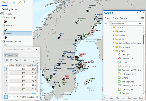
Figure 3.5 Example output from Project 3, viewed in Pro.
The above requirements are sufficient for receiving 90% of the credit on this assignment. The remaining 10% is reserved for "Over and above" efforts, such as making a script tool, or extending the script to handle multiple target countries, other combinations of fields and queries, etc. For these over and above efforts, we prefer that you submit two copies of the script: one with the basic functionality and one with the extended functionality. This will make it more likely that you'll receive the base credit if something fails with your over and above coding.
Deliverables
Deliverables for this project are as follows:
- The source .py file containing your script
- A short writeup (about 300 words) describing how you approached the project, how you successfully dealt with any roadblocks, and what you learned along the way. You should include which requirements you met, or failed to meet. If you added some of the "over and above" efforts, please point these out, so the grader can look for them.
You do not have to create a script tool for this assignment; you can hard-code the initial parameters. Nevertheless, put all the parameters at the top so they can be easily manipulated by whoever tests the script.
Once you get everything working, creating a script tool is a good way to achieve the "over and above" credit for this assignment. If you do this, then please zip all supporting files before placing them in the drop box.
Notes about the data
Take a look at the provided datasets in Pro, particularly the attribute tables. The nhlrosters shapefile contains a field called "position" that provides the values you need to examine (RW = Right Wing, LW = Left Wing, C = Center, D = Defenseman, G = Goaltender). As mentioned, you've been asked to extract the forward positions (RW, LW, and C) to new shapefiles, but you want to write a script that's capable of handling some other combination of positions, too. There are several other fields that offer the potential for interesting queries as well, if you're looking for over and above ideas.
The Countries_WGS84 shapefile has a field called "CNTRY_NAME". You can make an attribute selection on this field to select Sweden, then follow that up with a spatial selection to grab all the players that fall within this country. Finally, narrow down those players to just the ones that play the desired position.
Tips
Once you've selected Swedish players at the desired position, use the Copy Features [23] tool to save the selected features into a new feature class, in the same fashion as in the practice exercises.
Take this project one step at a time. It's probably easiest to tackle the extraction-into-shapefile portion first. Once you have all the new position shapefiles created, go through them one by one, use the "Add Field" tool to add the "height_cm" and "weight_kg" fields, followed by an UpdateCursor to loop through all rows and populate these new fields with appropriate values.
It might be easiest to get the whole process working with a single position, then add the loop for all the positions later after you have finalized all the other script logic.
The height field is of type Text to allow for the ' and " characters. The string slicing notation covered earlier in the course can be used to obtain the feet and inches components of the player height. Use the inches to centimeters formula shown above to compute the height in metric units.
For the purposes of this exercise, don't worry about capturing points that fall barely outside the edge of the boundary (e.g., points in coastal cities that appear in the ocean). To capture all these in real life, you would just need to obtain a higher resolution boundary file. The code would be the same.
You should be able to complete this exercise in about 50 lines of code (including whitespace and comments). If your code gets much longer than this, you are probably missing an easier way.