Geographic Phenomena: Models

Geographic Phenomena: Models

When conceptualizing the geographic phenomena we want to map, it is important to consider the best way that these phenomena can be modeled. In general, we can categorize the best model for a given phenomenon as existing somewhere along two continuums: (1) from discrete to continuous, and (2) from smooth to abrupt.

You likely learned the difference between discrete (e.g., as shown by a histogram) and continuous (e.g., as shown by the bell curve) variables in an introductory statistics course. The distinction in cartography is similar.

Discrete phenomena have well-defined boundaries: they occur at specific locations, with space in between. Examples include people, cars, houses, hospitals, and roads.

Continuous phenomena, conversely, have ill-defined or irrelevant boundaries. Examples include temperature, air quality, and elevation.

Phenomena can also—independent of their classification as discrete or continuous—be considered either smooth or abrupt.

Smooth phenomena are those that change gradually over geographic space. Examples include precipitation levels and solid aridity: they vary by location but do not typically change abruptly at geographic bounds. 

Abrupt phenomena do change suddenly at a geographic boundaries, whether physical or cultural. Often, phenomena are not clearly smooth or abrupt, but fall somewhere in between. The amount of pesticides in soil, for example, might vary somewhat continuously over space, but change rather abruptly at political boundaries (e.g., due to changing government regulations).

Figure 3.3.1 Discrete vs. Continuous; Abrupt vs. Smooth.

Credit: (MacEachren 1992)

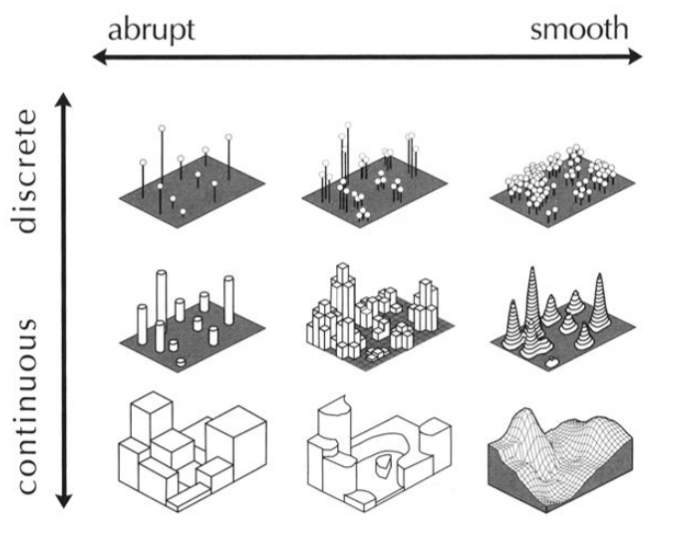
Figure 3.3.1 illustrates various surfaces used to represent geographic phenomena throughout the discrete to continuous and abrupt to smooth continuums. Keep this idea of a continuum in mind—geographic phenomena often cannot be classified into neat categories, and it is typically more fruitful to think of them as “more continuous” or “more discrete” than to try and fit them into a box.

Figure 3.3.2 Map representations that match the phenomena in Figure 3.3.1 above

Credit: (MacEachren 1992)

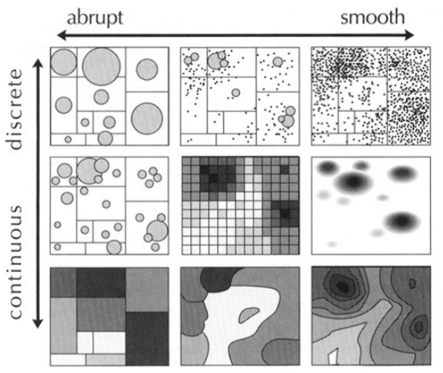
Figure 3.3.2 above shows different map representations that are suited to mapping the geographic phenomena located at these relative positions along the continuous-discrete and abrupt-smooth continua. We will discuss the appropriateness of various thematic mapping methods further later in this lesson.