3D Maps

3D Maps

Similar to how new web-based technologies have made it easier to design interactive and animated maps, technological advancements have altered mapmaking in another, related way—enabling more realistic depictions of the real world through more accessible 3D-mapping tools and virtual/augmented reality.

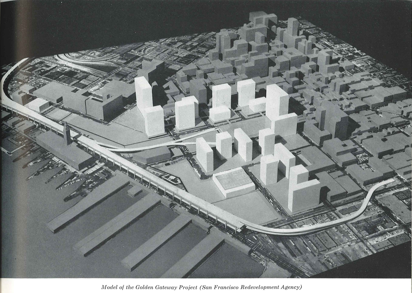
Three-dimensional visualizations have long been used to create city models (e.g., Figure 8.7.1) and similar models of Earth’s terrain or built environment. As we discussed in Lesson 6, these models are useful in that they provide a realistic view of the environment, but their realism and complexity often come at a cost. For example, the oblique view inherently obstructs some of the scene (e.g., locations behind tall buildings), and physical models are typically not built to scale.

Figure 8.7.1 A Model of the Golden Gateway Project from the San Francisco Redevelopment Agency (1960).

Credit: Eric Fischer, CC BY 2.0

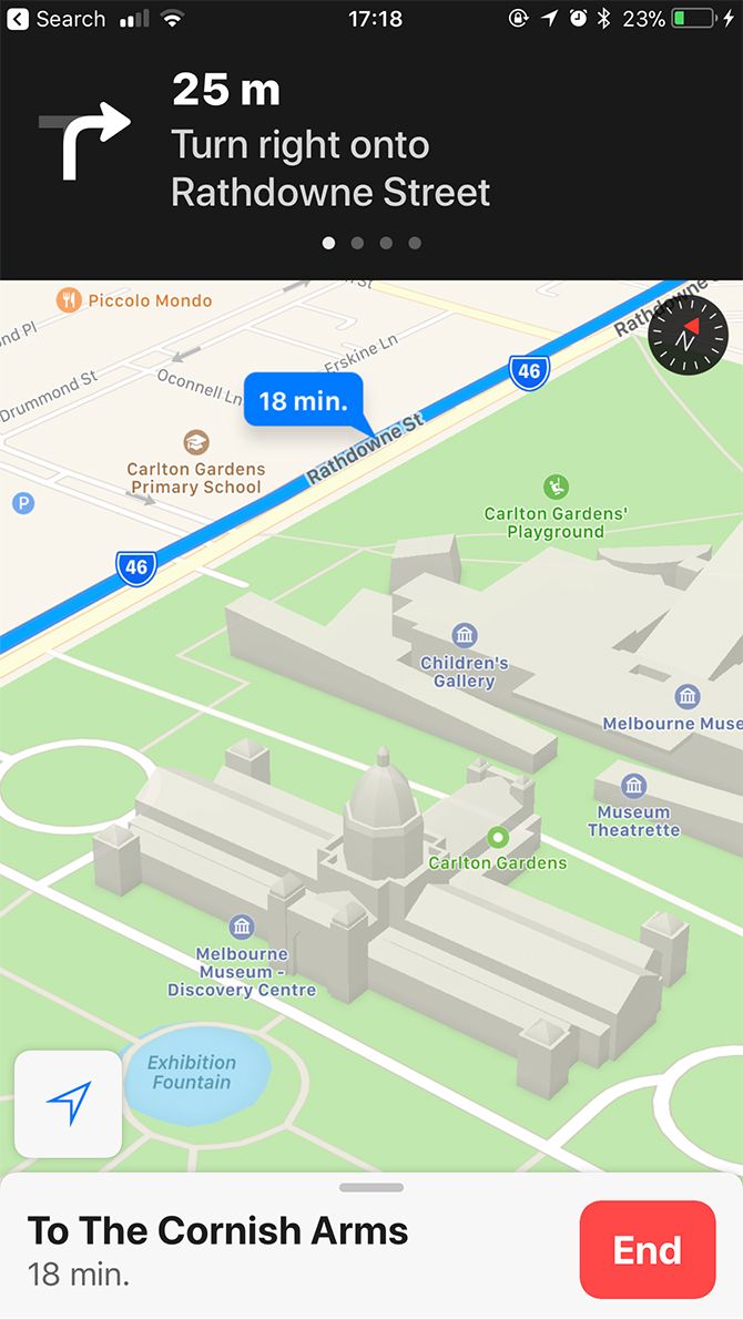
In the past, creating complex 3D digital visualizations and physical models came at a near-prohibitory cost. Yet recent increases in the computational power of mainstream computers and new software tools have reduced the time, capital, and expertise required to create three-dimensional maps. Naturally, this has encouraged cartographers to make more of them. The inclusion of 3D visuals in mapping tools has become increasingly widespread—realistic modeling of buildings can now be seen, for example, in popular mapping applications such as Apple Maps.

Increasing interest in and availability of 3D mapping tools has also resulted in an increased use of extruded or perspective height as a visual variable. Unlike the 3D map examples above, perspective height uses a third dimension to encode a variable distinct from the actual physical height of a feature.

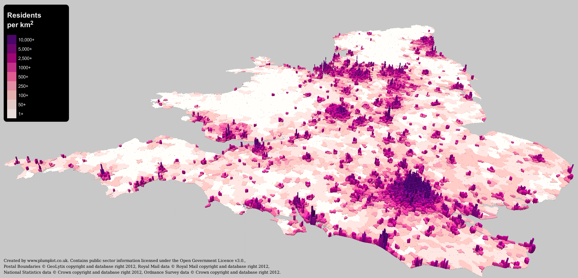
An example is shown below (Figure 8.7.2). This is a choropleth map that uses a multi-hue sequential color scheme to encode the population density of the United Kingdom by postal code. In addition to color, however, another visual variable is used—perspective height. Areas with higher densities are extruded from the map, giving them increased visual emphasis. The result is a map that portrays the look of a varied terrain—only instead of actual physical terrain, it visualizes the terrain of people across the landscape.

Figure 8.7.2 A map using extruded/perspective height to visually-encode population density in the UK.

Credit: plumplot

Similar to the visual depiction of uncertainty, an important question surrounds the use of 3D visualization: is it useful? The answer, as provided by recent cartographic research, is similar: it depends. Generally, studies have found that people enjoy using 3D maps more than their 2D counterparts. These studies also typically find, however, that people perform tasks less efficiently with 3D graphics than with simpler 2D visualizations (Smallman and John 2005).

There is no scientific consensus on whether 3D visualization tends to be helpful for users, and due to the context-dependence of such a question, it is unlikely that there will be an answer anytime soon. What the current state of research suggests is that 3D visualizations should be used with caution. In contexts where seconds count (e.g., emergency management; disaster response) for example, 3D visualization tools might be a risky option. In contexts where user enjoyment is of greater priority (e.g., in a university’s campus map), it might instead be an excellent choice.