Part I: Explore Publicly Available Wetlands Data & Historical Imagery

Part I, we will explore our study area and the time-series aerial photos used to digitize the vegetation data we will use in Part II. We will also look at two publicly available datasets specifically related to wetlands: the National Wetlands Inventory from the U.S. Fish & Wildlife Service and a more detailed wetlands inventory from a regional public agency called the Great Lakes Commission. In the process, we will explore several different data delivery options and sources in ArcGIS: Esri Map Packages, Esri Basemaps, ArcGIS Online Datasets, Web Map Services (WMS) from GIS Servers, and raw GIS files.

Familiarize Yourself with the Study Area and Set Up Your Map
1. Open the L3_Data folder you downloaded in the Lesson Data section. Double-click on the “Lesson3.mpkx” map package file. Designate your L3_Data folder as the unpacking location. This will open a map inside ArcGIS Pro with the study area boundary and historical imagery already loaded.
  
  You can share your own data and maps by creating a map package in ArcGIS Pro. Go to the Share tab, Package group, and select Map Package . The file can either be uploaded to ArcGIS Online or saved locally.
2. Set your Current Workspace and Scratch Workspace to your L3 folder by navigating to the Analysis tab, Geoprocessing group, Environments . Make sure to read the associated help topics about “Current Workspace” and “Scratch Workspace.”
  
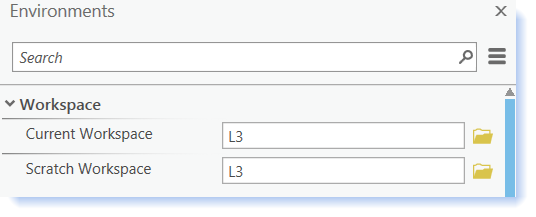
  Setting your Current Workspace allows you to customize the location of where output files created during geoprocessing steps are saved. By default, files will be saved at …My Documents\ArcGIS.
  
  To easily access information related to geoprocessing parameters and environments in ArcGIS: Click on the information icon which will open a dialog window with information about usage and options. It is also a good idea to read the help information related to tools you are not familiar with (click or go to the Project tab > Help).
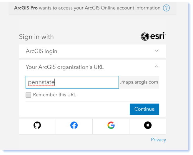
3. Add the “Open Street Map” ArcGIS Online Service (go to the Map tab, Layer group, click on Basemap > select OpenStreetMap) so you can tell where the study area is located in relation to the other places. You may need to refresh your map for the Basemap to load. (You need to be connected to the Internet and Signed In to the PSU AGO Organization using your WebAccess account information).
4. Use the Explore tool found on the Map tab, in the Navigate group to take a look at the study site and the surrounding area. What is the nearest major city? How far away is the site from the state border with Michigan?
5. Turn off the Basemap, as this can slow down the drawing speed of your map in late steps. Save your project.
Explore Historical and Recent Aerial Photos
1. Zoom to the study area boundary by right-clicking on it in the Contents pane > Zoom to Layer.
2. Turn on the “2005” layer in the Contents pane. This is a Color Infrared (CIR) image. Notice the information on the edge of the scanned film showing the date, location, and scale of the original image.
3. Turn on the “1973” and “1962” images. These images are black and white, a common format before 2000.
4. Compare the three images by turning them on and off and viewing them at a number of different scales: 1:15,000, 1:10,000, and 1:5,000. Try navigating to different locations within the study area. What differences do you notice between the three images?
  
  Take a minute to look at the swipe and flicker tools available on the Raster Layer, Appearance tab, Compare group (be sure an image is highlighted in the Contents pane) These tools can be useful for temporal change detection (especially of satellite images or air photographs that were taken at different times of the same location), data quality comparison, and other scenarios where you want to visually compare the differences between two layers in your map. Swipe allows you to interactively reveal what is underneath a particular layer; Flicker flashes layers on and off at the rate you specify. You can read more about these tools in Esri help.
5. The photos that were used to create the detailed vegetation data we will use in Part II all show the study area in the past. Let’s take a look at more current imagery and see if we notice any changes in the vegetation. We’ll use an image from 2018 to 2020 from the National Agricultural Imagery Program (NAIP).
6. We can add ArcGIS Online data to the Map by going to the Map tab, Layer group, Add Data > Data. Under Portal, click ArcGIS Online.
7. Search for USA NAIP Imagery. Click OK.
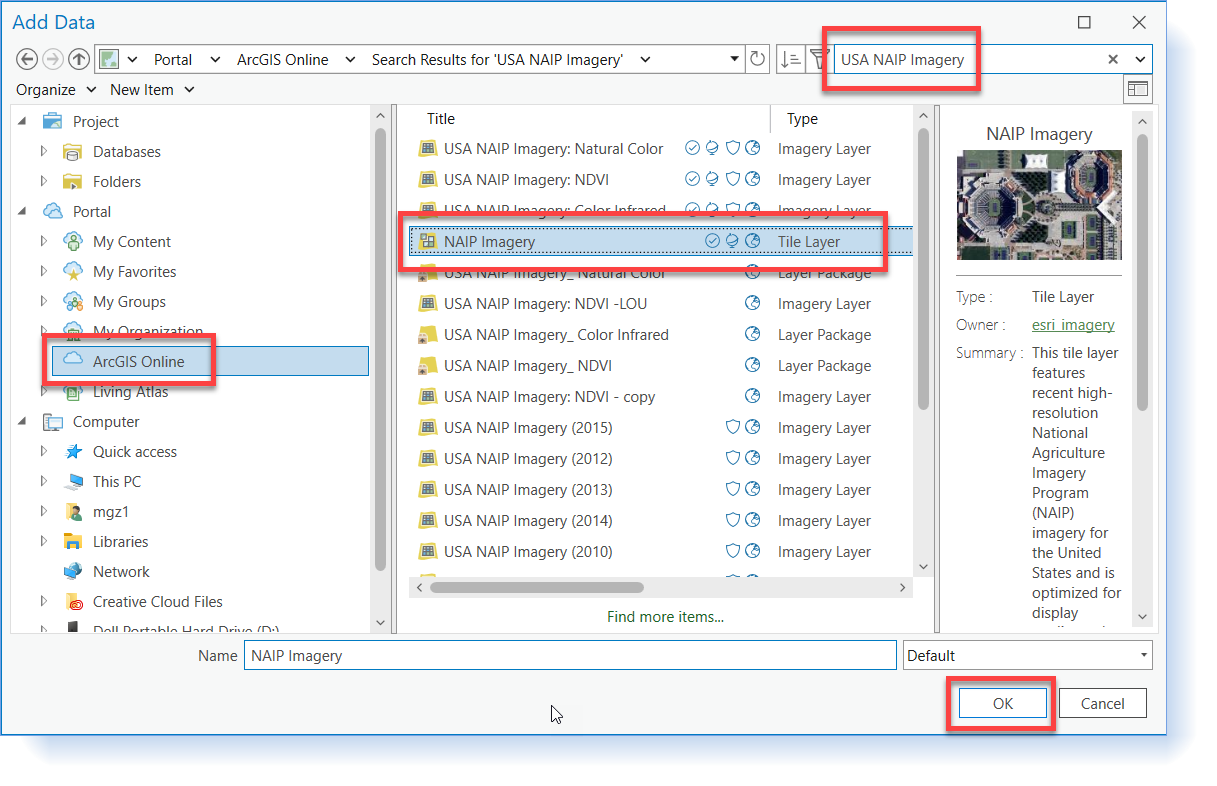
8. The USA NAIP Imagery layer will be added to the Contents pane.
9. Compare the NAIP Imagery with the historical aerials. What types of changes do you see? Notice that the NAIP Imagery is more natural in color, which is a bit easier to interpret (as compared to color infrared and black-and-white formats).
10. Turn off the imagery layers in the Contents pane and save your project.
Add the boundaries of the Fish & Wildlife Service Wildlife Refuges to your map
1. Again go to the Map tab, Layer group, Add Data > Data. Under Portal, click ArcGIS Online.
2. In the ArcGIS Online search window, type “national wildlife refuges” Review the datasets that match the search. Locate the "National Wildlife Refuges” dataset in the results.
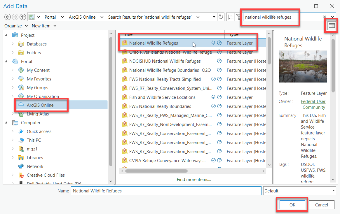
3. Click on the "Details" button to review the metadata. Notice that this data is a Feature Layer and was last modified on 7/25/2022. Click OK to add the layer to the Map.
4. Drag the study site boundary to the top of the Contents pane so you can see the site boundary on top of the feature service.
5. Zoom out to 1:250,000 so that you can see the various federal lands in the vicinity. The refuge is shown as a pinkish-filled polygon, which means it is a Great Lakes National Wildlife Refuge. Use the explore tool to click on the feature and identify the refuge's name.
6. Notice how the lesson study area only covers a portion of the whole refuge. The study site boundary represents the wetland areas within Ottawa National Wildlife Refuge that are hydraulically connected to Lake Erie. Some of the wetlands in the refuge are excluded from this area because they are hydraulically separated from Lake Erie by dikes and are therefore not susceptible to fluctuations in Lake Erie water levels. Other areas of the refuge are not wetlands.
7. Right-click on the “FWSBoundaries” layer name in the Contents pane > select Attribute table. Explore the attribute table. Are there any abbreviations you don’t understand?
8. Again, right-click on the “FWSBoundaries” layer > Properties > Source > Spatial Reference. Look at the spatial reference information. Is it the same as the study site? Does it match the data frame? (Right-click on StudyArea in the Contents pane > Properties > Coordinate Systems). Note: You may experience errors editing a data layer if it does not match that of the data frame.
Create a new shapefile of the Ottawa National Wildlife Refuge Boundary
1. Right now, the refuge boundaries on our map are part of a feature layer. We want to create a new shapefile from just a portion of the records so we can customize it for our study site.
2. Open the FWSBoundaries attribute table. Click on the “Select by Attributes” icon .
3. Create a new selection expression to select all of the polygons within the Ottawa National Wildlife Refuge Where "Organization Name" is equal to "Ottawa National Wildlife Refuge". Apply the expression. You should have 1 of 574 records selected. Close the attribute table. Notice that the polygon is a multipart feature, or it has more than one part but is defined as one feature because it references one set of attributes. Confirm this by viewing the attribute table.
4. Right-click on the layer in the Contents pane and click Data > Export Features. Export the selected features to a new shapefile called “OttawaNWR.shp” to your L3 folder. Make sure to go to the Environments tab in the Export Features dialog to establish the Output Coordinates as the same coordinate system as the Current Map [Study Area], or you may not be able to edit this data later on in the lesson.
5. The “OttawaNWR” shapefile will be added to your map. Verify the Coordinate System (Properties > Source > Spatial Reference) is the same as the StudyArea Map. Remove the “FWSBoudaries” dataset from your map and save the project.
6. Save your project.
Download and Explore the National Wetlands Inventory (NWI) Data
1. Connect to the National Wetlands Inventory data service. Go to the Insert tab, Project group, and click on Connections > Server > New WMS Server > Copy and paste the URL: https://www.fws.gov/wetlandsmapservice/services/Wetlands/MapServer/WMSServer? and click OK.
2. Go to the Map tab, Layer group, Add Data > Data. (Note: If you cannot view the layer using Add Data, try dragging the wetland layer from the Catalog pane > Project > Servers to the Map).
3. Under the Project folder, click on Servers. Double-click on WMS (www.fws.gov.wms) > WMS > Layers. Highlight the Wetlands layer and click OK to add the data set to your map. The layer will be added to the Contents pane and will be named WMS > Wetlands.
4. Drag the WMS Wetlands layer toward the top of the Contents pane but under the Study_Site layer. Zoom to the study area layer and explore the data.
5. Use the Explore tool from the Map tab to see what information is included with the layer. Notice that you can’t view an attribute table like you could with the feature layers.
6. According to the metadata, “the data are intended for use with base maps and digital aerial photography at a scale of 1:12,000 or smaller. Due to the scale, the primary intended use is for regional and watershed data display and analysis, rather than specific project data analysis.”
7. Unfortunately, the data does not contain enough detail to help us analyze vegetation changes in a specific wetland. It also does not allow us to study changes over time.
8. Turn off the “WMS” layer in the Contents pane and save your project.
Explore the Great Lakes Coastal Wetland Inventory Data
1. Read a quick description of the data at Great Lakes Commission (scroll down to the "Links to Inventory and Metadata" heading). Notice the link to the product metadata provided on the site. We are going to use one file from this site called, “the complete polygon coverage in shapefile format.”
2. Download the data zip file from the site or from the Lesson Data page (glcwc_cwi_polygons.zip - 12.46 MB), save it in your L3 folder, and unzip the file.
3. Add the “glcwc_cwi_polygon” shapefile to your map.
4. Open the attribute table and explore the available information. Notice how there is significantly more information than the previous wetland datasets we reviewed.
5. The “HGM_CLS1” and “HGM_CLS2” attributes show the wetland classification codes. You can read detailed descriptions of these codes in the “Great Lakes Coastal Wetlands" (enhanced metadata) document.
6. Right-click on the “glcwc_cwi_polygon” shapefile in the Contents pane > Zoom to Layer. It is difficult to see any detail.
7. Zoom back to the Study_Site layer. Do you see any wetlands inside the Ottawa National Wildlife Refuge that are not inside our study site boundary? You may need to move the Study_Site boundary layer and OttawaNWR layers to the top of your Contents pane.
8. Turn the layer off in your Contents pane and save your project.
9. The Great Lakes Coastal Wetland Inventory provides much more detailed attribute information than the National Wetlands Inventory. However, it still doesn’t provide the time-series information we need to answer our research questions. For time-series data, we need to look at yet another data set.