Part I: Create Shapefile from Field Data Tables
In Part I, we will create the shapefile we will use to interpolate our data (a point shapefile of plots with the total carbon as an attribute). To create this, we start with the two CSV files "GPS.csv" and "Tree _Measurements.csv".
-
Familiarize Yourself with the Study Area
- Create a New Map and save your project to the L6 folder without creating a new folder for the project.
- Add the parcel boundary and forest boundary from your L6Data folder to your Map.
- Change the parcel and forest boundaries symbols to hollow outlines.
- Go back to the Map tab and add the "OpenStreetMap" and “Imagery Hybrid” Basemaps to your Map.
- Use the Explore tool to pan and zoom within the surrounding area. Notice how the imagery shows that only the southern portion of the parcel is forested.

How far is the study forest from the city of Ann Arbor, MI or State College, PA? What is the surrounding land used for (commercial, agriculture, residential, etc.)?
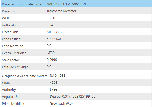
- Confirm the coordinate system of the Map is set to “NAD 1983 UTM Zone 16N.” If yours does not match, right-click on the Lesson 6 Map in the Contents pane > Properties > Coordinate System > Projected Coordinate Systems Folder > UTM > NAD 83 > NAD 1983 UTM Zone 16N. Save your project to lock in the settings.
-
Create Plot Shapefile from GPS Data Table
- Add the "GPS.csv" file from your L6Data folder to your map and explore the attributes.
- Open the table and explore the attributes. What spatial reference do you think the x and y coordinates refer to?
- Right-click on the GPS table in the Contents pane > XY Table To Point
- X Field: LONGITUDE
- Y Field: LATITUDE
- Z Field: <None> (since we are not interested in height)
- Coordinate System: GCS_WGS_1984

- Right-click on the "GPS_XYTabletoPoint" layer in the Contents pane > Data > Export Features and export to a new shapefile in your L6 folder. Name it "Plots." Make sure you establish the output coordinate system under Environments as NAD_1983_UTM_Zone_16N.
- The "Plots" shapefile will be added to the Map, remove the GPS_XYTabletoPoint layer, and the GPS table from your Contents pane and Save the project.
Make sure you have the correct answer before moving on to the next step.
Check the Properties > Source Tab > Spatial Reference to make sure the Plot shapefile was projected correctly to NAD 183 UTM Zone 16N. If your projection doesn’t match, make sure you remove the base maps, and choose the coordinate system of the Map.

Make sure you have the correct answer before moving on to the next step.
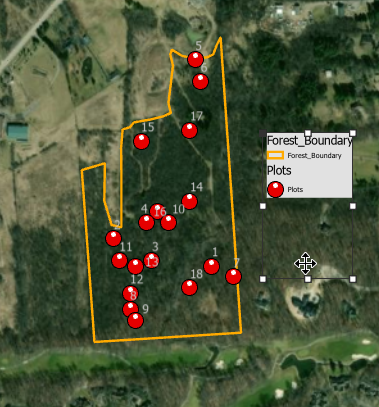
Check the location of your plots by comparing your plot shapefile to the map below. Note: Your map will not look exactly like this by default. I changed the symbology of the points, added labels of Plot ID's, and added the Imagery layer in the background to make it easier to compare your data to the example. If you add the imagery base map again, make sure you remove it from your map and Save before moving on to the next step.
-
Calculate the Carbon Sequestered by Each Tree
- Add the tree measurements CSV file from your L6Data folder to your map and explore the attributes. What does DBH mean?
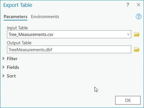
- We need to add several new fields to the table to calculate the carbon values for each tree. ArcGIS will not allow you to add new fields to a CSV file. Export it to a .dbf file of the same name using the export option listed in the dropdown menu in the upper left corner of the attribute table. Make sure to select the file type as dBASE table so it has the “.dbf” extension. Add the resultant file to your map.
- Remove the "Tree_Measurements" CSV file from your Map and Save the project.

We are going to use a somewhat general set of equations to estimate the carbon stored in each tree. For this lesson, we do not need a high level of accuracy. The important part is to demonstrate the concept of how one can calculate carbon credits using GIS. You can read more about the method we will use at: How to calculate the amount of CO2 sequestered in a tree per year.
There are more sophisticated methods you can use that take into account the tree species, age, climate, and other factors. The paper, “Methods for Calculating Forest Ecosystem and Harvested Carbon with Standard Estimates for Forest Types of the United States” highlights an example of a more complex methodology. An example of a simpler method is highlighted in the “Landowner’s Guide to Determining Weight and Value of Standing Pine Trees”.
- Add 7 new double fields to the Tree_Measurements dbf table. Save
 the changes after you have added the fields. Use the names below:
- DBH_in (this is to convert units from cm to in)
- Height_ft (this is to convert units from m to ft)
- Wa_lbs (above ground tree weight)
- Wt_lbs (total tree weight with roots)
- Wd_lbs (dry tree weight)
- Wc_lbs (weight of carbon)
- Ws_lbs (weight of carbon dioxide sequestered)
- Use the calculate field tool and the equations below to populate the new fields from step d.
Variable Description Units Equation D Measured tree diameter (DBH) Inches See Tree Measurements Table (be careful with your units here). H Measured tree height Feet See Tree Measurements Table (be careful with your units here). Wa Total above-ground weight of the tree (w/o roots) Pounds Wa = 0.15D2 *H Wt Total weight of the tree and roots Pounds Wt = 1.2 Wa Wd Dry weight of the tree Pounds Wd = 0.725Wt Wc Weight of carbon in the tree Pounds Wc = 0.5Wd Ws Weight of carbon dioxide sequestered in the tree Pounds Ws=3.6663Wc Tips for Success:
- Don’t forget to convert units when necessary. Check Online Conversion.com if you are unsure of the conversion equations. Round the conversion factors to the nearest 4 decimal places (e.g., 0.3937007874 = 0.3937). What is the conversion factor for meters to feet?
- Make sure to use double as the data type.
- Remember that you have the option to undo.
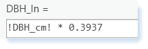
- To calculate D2 in the Python 3, multiply D * D or D**2 (e.g., 0.15 * !DBH_In!**2 * !Height_ft!)
- The example below shows the equation you would type into the calculate field (Python 3) to convert the DBH values from centimeters to inches.
Make sure you have the correct answer before moving on to the next step.
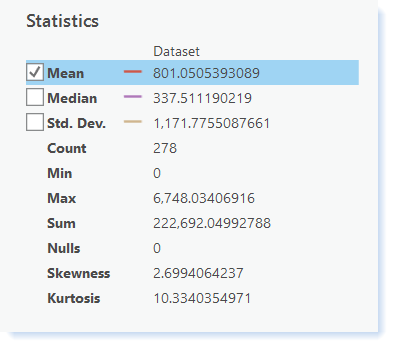
Compare your data with the summary statistics below for the "Ws" variable.
 Click here for an accessible version of the data above
Statistics Shown in the image above Mean 801.0505393089 Median 337.511190219 Std. Dev. 1,171.7755087661 Count 278 Min 0 Max 6,748.03406916 Sum 222,692.04992788 Nulls 0 Skewness 2.6994064237 Kurtosis 10.3340354971 If your data does not match this, go back and redo your calculations. Pay special attention to unit conversations (make sure to round to the nearest 4 decimal places), data types of the fields you used, and typos in equations.
-
Combine the Carbon Calculations with the Plot Shapefile
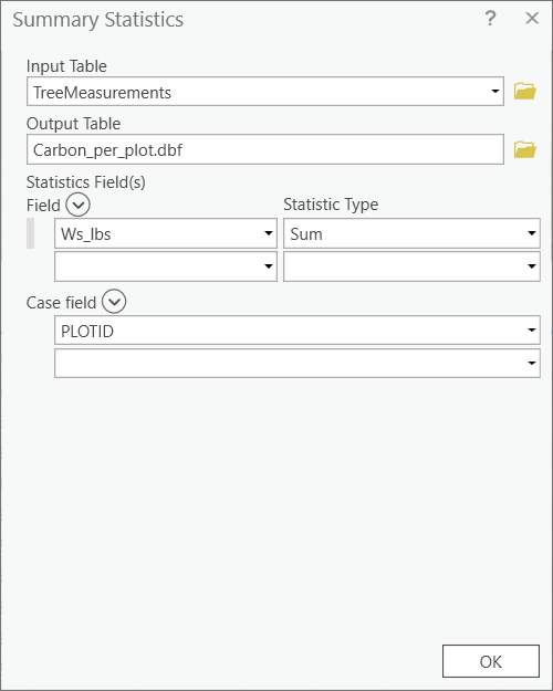
Ultimately, we want to join the calculations from Step 3 to the plot shapefile we created in Step 2. However, we can’t do this directly, because there is more than one entry in the tree measurement table for each plot in the shapefile. We know this is true because there are 278 trees but only 18 plots. Before we can join the two files, we need to summarize the tree data to the plot level.- Calculate the total carbon sequestered per plot. Open the "Tree_Measurement" dbf table. Right-click on the "PLOTID" field>Summarize. Use the settings shown in the following figure. Make sure the extension is a .dbf file.
- The "Carbon_per_plot" table will be added to your map. Notice there are only 18 records now instead of 278. The "FREQUENCY" is the number of trees within each plot. (Now is a good time to change the field alias to “Number _Trees” so you remember what this means later on. Right-click on the field > Field > alias.) The "Sum_Ws_lbs" is the total carbon sequestered for all trees within the plot.
- Now we know the total carbon sequestered for each plot. However, we still need to normalize this data before we can interpolate it since we’re estimating carbon values across the entire area where there aren’t any additional plots. Because the diameter of each plot is 10 meters, we know the area of each plot is 78.5 square meters. By dividing each carbon total by this area, we derive a “carbon per square meter” value, which can be interpolated across the entire study area.
- Add a new double field named "c_lbsqm" to the "Carbon_per_plot" table. Calculate the pounds of carbon sequestered per square meter for each plot.
Make sure you have the correct answer before moving on to the next step.
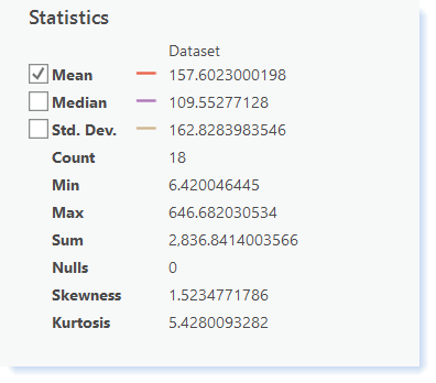
Compare your data with the summary statistics below for the "c_lbsqm" variable.
 Click here for an accessible version of the data above
Statistics Shown in the image above Mean 157.6023000198 Median 109.55277128 Std. Dev. 162.8283983546 Count 18 Min 6.420046445 Max 646.682030534 Sum 2,836.8414003566 Nulls 0 Skewness 1.5234771786 Kurtosis 5.4280093282 If your data does not match this, go back and redo your calculations.
- Join the "Carbon_per_plot" table with the "Plots" shapefile based on the PLOTID field. Open the attribute table to make sure your join worked properly.
- Export features to a new shapefile in your L6 folder named "Plots_carbon.shp" Be sure the new shapefile is added to your Map.
- Remove the "Tree_Measurements" table, "Carbon_per_plot" table, and "Plots" shapefile.
- Save the project.
- Calculate the total carbon sequestered per plot. Open the "Tree_Measurement" dbf table. Right-click on the "PLOTID" field>Summarize. Use the settings shown in the following figure. Make sure the extension is a .dbf file.