Part I: Acquire Data and Organize the Map

Part I: Acquire Data and Organize the Map

In Part I, we will explore and obtain publicly available datasets from the Pennsylvania Spatial Data Access (PASDA ) website. We will also review the private data for this lesson and organize the map for analysis.

1. Download the Historical Land Use Data

   1. Download the data from the Lesson Data page and extract the files.
   2. Go to Pennsylvania Spatial Data Access.
   3. Under "Search Data by Keyword" enter "PAMAP Land Cover". 
   4. Locate "PAMAP Program Land Cover for Pennsylvania, 2005" and click on the Download name under data description.
   5. Review the metadata by clicking the Metadata link.
   6. Notice how the data is available both as a direct download and as an API map service. The map service will load very quickly in ArcGIS. However, it only provides a picture of the data, so we can't input it into our GIS analysis. 
   7. Click "Download." Note the large download size (approximately 167 MB) and allow sufficient time for download.
      *If you are using Chrome, you may need to switch to Microsoft Edge and proceed by right-clicking the Download button and click on "Open link in new tab" in order to download the data file. 
   8. It is helpful to come up with meaningful, standardized names when using datasets from multiple sources since different groups will usually follow different naming conventions. Rename the zip file from “palulc_05_utm18_nad83.zip” to “LU_2005.zip” so it matches the other dataset in our lesson (LU_1978). 
   9. Save the zip file in your " L5Data” folder and extract it. 
      

      When working with raster data that you have downloaded, you need to be careful when placing it on your computer. Many raster datasets have an associated Info folder that contains critical reference information. The files contained within this folder are numerically named based on the particular order in which they were originally created. As a result, it is possible that different raster datasets have identically named reference files within this folder.

      It is important to note that although these files may have the same name, they do not contain the same information. Therefore, it is possible to corrupt your data if you overwrite one set of a raster dataset’s files with another’s. You can avoid this potential problem by creating new folders for each dataset and extracting each zip file within its own folder.

2. Organize Your Map and Familiarize Yourself with the Study Area and Data

   1. Create a New Map and save your project to the L5Data folder without creating a new folder for the project.
   2. Add the "Study_Area" and "Counties" shapefiles to your map. Change the symbology for the features in each layer to hollow outlines.
   3. Add the "OpenStreetMap" ArcGIS Basemap to your map.
   4. Use the zoom and pan tools to explore the surrounding area.
      

      What are the largest towns within the study area? Where is the study site in relation to the overall area of Pennsylvania?
      
      
       

   5. Confirm that the coordinate system of the map is “NAD_1983_Albers.”
   6. Save your project.
   7. Open a Catalog pane (Go to View tab, from the Window group > Catalog Pane) and explore the contents of the “LU_1978” and “LU_2005” folders. Notice that there are actually several different raster files in the 2005 folder. One is in a TIFF format (palulc_05) and the remaining two are in GRID format. We will use the dataset found in the "AlbersPA83" folder since it is already in the format and projection we need for this analysis.
      
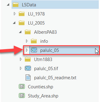
   8. Add the "LU_1978" and "palulc_05" rasters to your map. If prompted with "Would you like to create pyramids?" select "No."
   9. Familiarize yourself with the contents of each data set to see similarities and differences between them. In particular, pay attention to the codes listed in the "VALUE" field of each attribute table. These are coded values representing land cover types, similar to the VEG_IDs from Lessons 3 and 4.
      

      Raster attribute tables are different from vector attribute tables. Unlike with vector files, each unique value is only listed once.

      
      

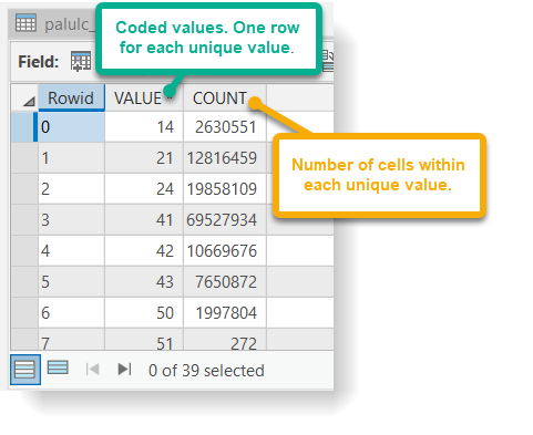
      Do all of the land cover raster datasets have the same number of coded values? How many unique codes does each raster dataset contain? Are any of the codes the same? Do they have the same extent and cell size? Do all of the datasets have the same spatial reference information?