Part II: Customize the Land Cover Data and Perform the Analysis
We want to figure out how land use has changed between 1978 and 2005 for several counties in southeastern Pennsylvania. We are mainly interested in the urbanization of agricultural and forested areas. You may have noticed that the land cover categories and coded values are different for the 1978 and 2005 datasets. Since we are interested in comparing land use change, we will need to standardize these categories before we can compare them. We also want to remove extraneous information from our datasets to make them easier to work with. We will use the Reclassification Tool in Spatial Analyst to perform both of these tasks simultaneously.
We will reclassify both of the input raster data layers using the standardized codes below. Codes 1, 2, and 3 collapse the existing detailed categories into broader categories. The "NODATA" (ALL CAPS) category allows us to ignore all of the land cover categories that we are not using in our analysis.
| Value | Category |
|---|---|
| 1 | Developed Land |
| 2 | Agricultural Land |
| 3 | Forested Land |
| NODATA | All Other Values |
The tables below show the original land cover codes from the 1978 and 2005 land cover grids, associated descriptions, and the new codes we will use to reclassify the data.
| Original value | Original Category | NEW Reclass Value |
|---|---|---|
| 11 | Residential | 1 |
| 12 | Commercial and Services | 1 |
| 13 | Industrial | 1 |
| 14 | Transportation, Communications... | 1 |
| 15 | Industrial and Commercial Complexes | 1 |
| 16 | Mixed Urban or Built-up Land | 1 |
| 17 | Other Urban or Built-up Land | 1 |
| 21 | Cropland and Pasture | 2 |
| 22 | Orchards, Groves, Vineyards | 2 |
| 23 | Confined Feeding Operations | 2 |
| 24 | Other Agricultural Land | 2 |
| 31 | Herbaceous Rangeland | NODATA |
| 32 | Shrub and Brush Rangeland | NODATA |
| 33 | Mixed Rangeland | NODATA |
| 41 | Deciduous Forest Land | 3 |
| 42 | Evergreen Forest Land | 3 |
| 43 | Mixed Forest Land | 3 |
| 51 | Streams and Canals | NODATA |
| 52 | Lakes | NODATA |
| 53 | Reservoirs | NODATA |
| 54 | Bays and Estuaries | NODATA |
| 61 | Forested Wetland | 3 |
| 62 | Non-forested Wetland | NODATA |
| 72 | Beaches | NODATA |
| 73 | Sandy Areas other than Beaches | NODATA |
| 74 | Bare Exposed Rock | NODATA |
| 75 | Strip Mines, Quarries, and Gravel Pits | NODATA |
| 76 | Transitional Areas | NODATA |
| Original value | Original Category | NEW Reclass Value |
|---|---|---|
| 14 | Roads | 1 |
| 21 | Row Crops | 2 |
| 24 | Pasture/Grass | 2 |
| 41 | Deciduous Forest | 3 |
| 42 | Evergreen Forest | 3 |
| 43 | Mixed Deciduous and Evergreen | 3 |
| 50 | Water | NODATA |
| 51 | Streams and Canals | NODATA |
| 52 | Lakes | NODATA |
| 61 | Forested Wetlands | 3 |
| 62 | Emergent Wetlands | NODATA |
| 70 | Bare; Unclassified Urban/Mines, Exposed Rock, Other Unvegetated Surfaces | NODATA |
| 111 | Residential Land; 5-30% impervious | 1 |
| 112 | Residential Land; 31-74% impervious | 1 |
| 113 | Residential Land; 74% < impervious | 1 |
| 121 | Institutional/Industrial/Commercial Land; 5 - 30% impervious | 1 |
| 122 | Institutional/Industrial/Commercial Land; 31 - 74% impervious | 1 |
| 123 | Institutional/Industrial/Commercial Land; 74% < impervious | 1 |
| 124 | Airports | 1 |
| 241 | Golf Courses | 1 |
| 750 | Active Mines/Significantly Disturbed Mined Areas | NODATA |
| 1111 | Residential Land; 5 - 30% impervious; Deciduous Tree Cover | 1 |
| 1112 | Residential Land; 5 - 30% impervious; Evergreen Tree Cover | 1 |
| 1113 | Residential Land; 5 - 30% impervious; Mixed Tree Cover | 1 |
| 1121 | Residential Land; 31 - 74% impervious; Deciduous Tree Cover | 1 |
| 1122 | Residential Land; 31 - 74% impervious; Evergreen Tree Cover | 1 |
| 1123 | Residential Land; 31 - 74% impervious; Mixed Tree Cover | 1 |
| 1131 | Residential Land; 74% <impervious; Deciduous Tree Cover | 1 |
| 1132 | Residential Land; 74% <impervious; Evergreen Tree Cover | 1 |
| 1133 | Residential Land; 74% < impervious; Mixed Tree Cover | 1 |
| 1211 | Institutional/Industrial/Commercial Land; 5 - 30% impervious; Deciduous cover | 1 |
| 1212 | Institutional/Industrial/Commercial Land; 5 - 30% impervious; Evergreen tree cover | 1 |
| 1213 | Institutional/Industrial/Commercial Land; 5 - 30% impervious; Mixed tree cover | 1 |
| 1221 | Institutional/Industrial/Commercial Land; 31 - 74% impervious; Deciduous Tree Cover | 1 |
| 1222 | Institutional/Industrial/Commercial Land; 31 - 74% impervious; Evergreen Tree Cover | 1 |
| 1223 | Institutional/Industrial/Commercial Land; 31 - 74% impervious; Mixed Tree Cover | 1 |
| 1231 | Institutional/Industrial/Commercial Land; 74% < impervious; Deciduous tree cover | 1 |
| 1232 | Institutional/Industrial/Commercial Land; 74% < impervious; Evergreen tree cover | 1 |
| 1233 | Institutional/Industrial/Commercial Land; 74% < impervious; Mixed tree cover | 1 |
After all of the time periods share common land cover codes, we can calculate how much change has occurred in each category over time using the workflow below:
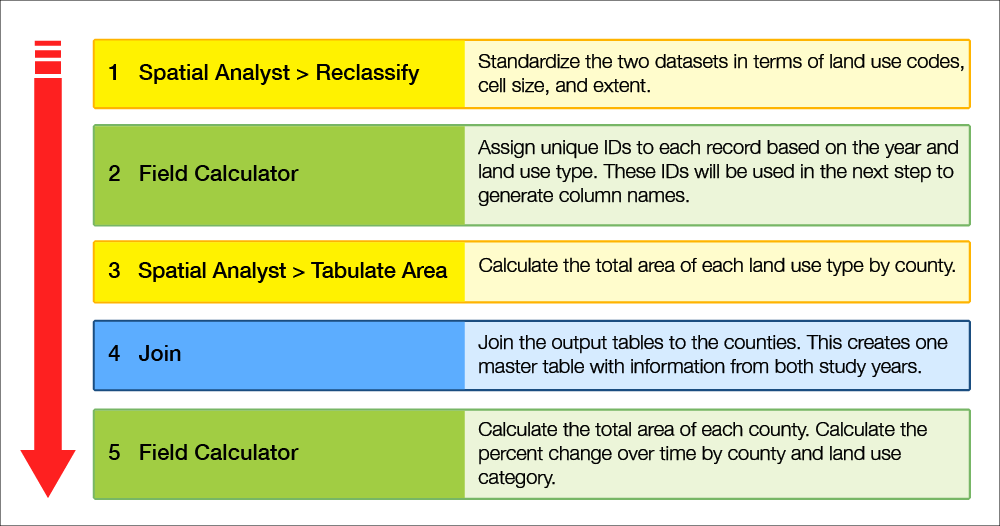
- Spatial Analyst > Reclassify: Standardize the two datasets in terms of land use codes, cell size and extent
- Field Calculator: Assign unique IDs to each record based on the year and land use type. These IDs will be used in the next step to generate column names.
- Spatial Analyst > Tabulate Area: Calculate the total area of each land use type by county
- Join: Join the output tables to the counties. This creates one master table with information from both study years.
- Field Calculator: Calculate the total area of each county. Calculate the percentage change over time by county and land use category.
-
Specify Geoprocessing Environment Settings

It is important to remember to double-check the environment settings within the Spatial Analyst tool pane, as ArcGIS sometimes ignores the global environment settings. A general rule of thumb is to always be certain of the environment settings used in your analysis, as they are critical to your results.
- Go to the Analysis tab, Geoprocessing group, Environments, verify that your workspace (Lesson 5 folder) and output coordinates (same as Study_Area) have been correctly set.
- We can remove portions of rasters by using the extent and mask settings. We’ll take advantage of this functionality to clip the two rasters to our study area.
- Under "Processing Extent", choose "Same as Layer Study_Area" as the extent.
- Under "Raster Analysis", choose the "Study_Area" as the mask.
- You typically want to use the same cell size as your coarsest dataset. Check the cell size of the 1978 and 2005 rasters (Properties > Source > Cell Size). Which one is the largest? Notice that both of the datasets have odd cell sizes with many decimal places. This is likely related to projection changes at some point during the preprocessing of the original data. We are going to pick "Maximum of Inputs".
- Finally, we want to ensure that we do not build pyramids for any layers. Pyramids will generalize data as you zoom out, which will reduce the visible accuracy of the displayed data. Scroll down to "Raster Storage", and uncheck Build.
- Click OK to save these settings. Save your project.
-
Reclassify the 1978 Land Use Data
- Within the Analysis tab, Geoprocessing group go to Tools > Toolboxes > Spatial Analyst Tools > Reclass > Reclassify.
- Verify the Reclassify tool Environments settings (i.e., Output Coordinates - "Study_Area", Processing Extent - "Same as Layer Study_Area", Raster Analysis - Cell Size "Maximum of Inputs", Mask "Study_Area")
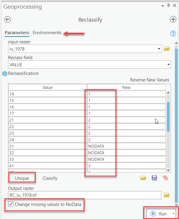
- Within the Parameters, Select "lu_1978" as the "Input raster" and "VALUE" as the "Reclass field."
- Click "Unique" to populate the "Values" column with the unique values in the dataset.
- Using the reclassification values given in Table 2, enter the appropriate values into the "New" column. Pay strict attention to the values you are entering to ensure proper reclassification.
- Name the new grid "RC_lu_1978.tif" and save it in your L5 folder.
Note: In ArcGIS, the default Output Raster format is a TIFF (.tif). - Check the "Change missing values to NoData" box.
- Click Run to perform the reclassification. Be patient as this may take a couple of moments depending on your computer’s configuration.
- If you’d like to review the progress, environment settings, and inputs, go to the Analysis tab, Geoprocessing group >History.
- "RC_lu_1978.tif" will be added to your map. Set the symbology so 1= red, 2= orange, and 3=green, and NoData = grey (Mask tab).
- Compare the output to the original raster. Right-click on the “lu_1978” layer in the Contents pane > Zoom to layer.
Notice how the extent setting we used clipped the raster to a much smaller area, and the mask setting we used assigned values of NoData to all of the areas that are both outside our study area boundary and within the extent.
Also, notice the grey areas within our study area. These are places that we reclassified the original land cover to "NoData." Keep in mind that you could also do the opposite of what we did – you can reclassify cells with starting values of "NoData" to other values.

Make sure you have the correct answer before moving on to the next step.
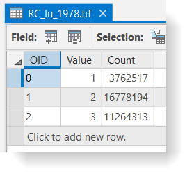
The cell counts in your RC_lu_1978.tif should match the examples below. If your data does not match this, go back and redo the previous step. You can double-check settings and rerun the tool in the Results window.
You’ll need right-click the RC_lu_1978.tif in Contents pane > Attribute table to see the Count attribute.
- Change the color of NoData back to “no color.”
- Since we no longer need the original land use layer, remove the lu_1978 grid from your map and Save the project.
-
Reclassify the 2005 Land Use Data
- Use the process from Step 2 and the values in Table 3 to reclassify "palulc_05” into a simplified land cover grid.
- Name the new grid "RC_LU_2005.tif"
- Add "LU_2005_RC" to your map and set the symbology so 1= red, 2= orange, and 3=green, and NoData = grey.
- Compare the output to the original raster. Right-click on the “lu_2005” layer in the Contents pane > Zoom to layer.

How did the extent, mask, and cell size settings affect the output raster? You can view the cell size settings by right-clicking on the output raster > Properties > Source > Cell Size.
Make sure you have the correct answer before moving on to the next step.
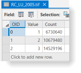
Your LU_2005_RC grid should match the example below. If your data does not match this, go back and redo the previous step.
- Change the color of NoData back to “no color.”
- Since we no longer need the original land cover layer, remove the "palulc_05" grid from your map and Save the project.
Since you know the cell size and number of cells with each unique value, you can easily calculate the total area within each land cover category for the entire study area. Note that you need to use the area of the cell, not the length, when making these calculations.
-
Add Unique Identifier
In the next step, we will use the "Tabulate Area" tool to create a table with the areas of each land cover type within each county. We will repeat this for both time periods. The "Tabulate Area" tool will automatically generate column names based on the values in the input table. Since we will have two datasets with the same land cover codes, we need to be able to keep track of each year’s corresponding table. To do this, we will add new fields to each reclassified raster attribute table and populate them with a combination of the study year and the land cover code.
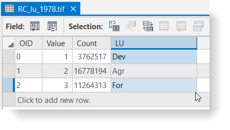
- Right now, the land covers are represented by arbitrary codes of 1, 2, and 3. We are going to assign more meaningful names (three letter abbreviations) so we don’t confuse the numeric codes later on. Open the RC_lu_1978.tif attribute table and add a new text field called “lu” with a length of 3.
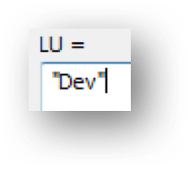
- Select the first row (VALUE = 1) and use the calculate field to assign a value of “Dev.”
- Repeat for the remaining rows as shown below and then Save your edits.
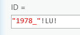
- Add a new text field named "ID" with a length of 8 (4 characters for the year, one character for a "_", and three characters for the land use abbreviations).
- Set the values of the ID field to be equal to "1978_"!LU!. This will create a unique ID for each land use code and year. For example, the first row has a value of Dev, so the ID field would be set to "1978_Dev".
- View the results to make sure your calculation worked as planned. Close the attribute table.
- Repeat for the 2005 data. Make sure you use the correct year in your calculations.
- Clear the selected features and save your map. (If you skip this step, future operations will only be run on the fields you have selected).
Make sure you have the correct answer before moving on to the next step.
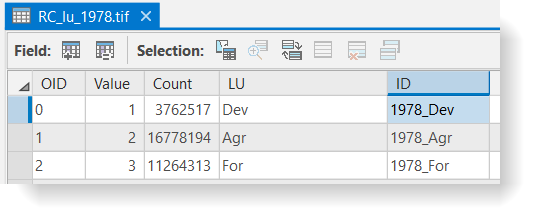
Your reclassified attribute tables should have their ID values populated as shown below. If your data does not match this, go back and redo the previous step.
 Click for a text alternative to the image above.
Accessible Version of Data Above, 1978 OID Value Count LU ID 0 1 3762517 DEV 1978_Dev 1 2 16778194 Agr 1978_Agr 2 3 11264313 For 1978_For 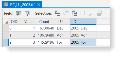 Click for a text alternative to the image above.
Accessible Version of Data Above, 2005 OID Value Count LU ID 0 1 6730640 Dev 2005_Dev 1 2 10679480 Agr 2005_Agr 2 3 14529196 For 2005_For
-
Tabulating Areas of the Land Use Grids
Now that we have reclassified the land cover data with standardized categories and created unique IDs, we can begin our land use change analysis. We need to calculate the area for each of the three land cover categories within each county for each time period. To do this, we will use the "Tabulate Area" tool. This tool calculates cross-tabulated areas between two datasets. This tool summarizes one dataset within regions specified by a second data set.
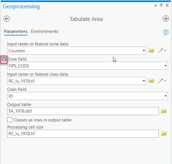
- Within the Analysis tab, Geoprocessing group go to Tools > Toolboxes > Spatial Analyst Tools > Zonal > Tabulate Area.
- Select "Counties" as the "Input raster or feature zone data" layer and "FIPS_CODE" as the "Zone field." The FIPS_CODE is a national naming convention system (similar to zip codes), that assigns a unique code to each county.
- Select RC_lu_1978.tif as the "Input raster or feature class data" layer and "ID" as the "Class field."
- Name the Output table "TA_1978.dbf" and save it in the L5 folder. Be sure to include the .dbf extension at the end of your file name to create a dBase table. Failure to add this file extension will result in an INFO table, which has different functionality than a DBF file. You will encounter trouble later in the lesson if you skip this small step.
- Make sure to read the embedded help topics about what each parameter controls.
- Leave the default processing cell size and click Run to tabulate the areas.
Open the "TA_1978.dbf" table in your map. Notice the names of the columns. What are the units of the tabulated areas?
- Repeat this process for the 2005 reclassified raster using "ID" for the class field. Name the output table "TA_2005.dbf.”
Make sure you have the correct answer before moving on to the next step.
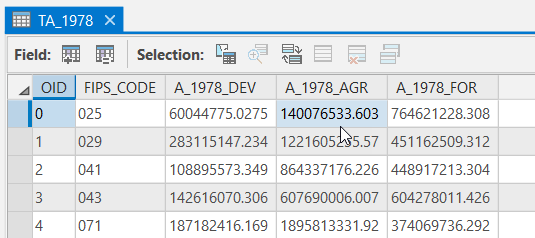
Your tabulated area tables should match the examples below. Both of the tables should have 19 records and 5 columns. If your data does not match this, go back and redo the previous step.
 Click for a text alternative to the image above.
Sample Data 1978 OID FIPS_CODE A_1978_Dev A_1978_AGR A_1978_FOR 0 025 60044775.0275 140076533.603 764621228.308 1 029 283115147.234 1221605255.57 451162509.312 2 041 108895573.345 864337176.226 448917213.30 3 043 142616070.306 607690006.007 604278011.426 4 071 187182416.169 1895813331.92 374069736.292 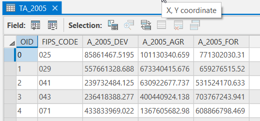 Click for a text alternative to the image above.
Sample Data 2005 OID FIPS_CODE A_2005_Dev A_2005_AGR A_2005_FOR 0 025 85861467.5195 101130340.659 771302030.31 1 029 557661328.688 673340415.676 659276515.52 2 041 239732484.125 630922677.737 531524170.633 3 043 236418388.277 400440924.138 703767243.941 4 071 433833969.022 1367605682.98
608866798.469
-
Create a Master Table of the Two Tabulate Area Tables
We will use the Join function to create a "master table” that contains the information from both of the Tabulate Area tables and the attributes of the counties. Since a joined table contains only virtually referenced information, we will export this dataset, thus permanently saving the joins.
- Right-click on the "Counties" shapefile and choose Joins and Relates > Add Join. Use the settings below and click "Validate" and then "OK". There may be a warning about the .dbf file not being indexed, it is OK to proceed.
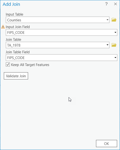
- Open the "Counties" attribute table to view the join. Notice how the FIPS_CODE’s match up with County Names.
- Right-click on the "Counties" shapefile again and create another join between the TA_2005 table based on the "FIPS_CODE." Open the "Counties" attribute table to view the second join. Your "Counties" attribute table should now have fourteen columns.
- You may notice that some of the field names are redundant. We will remove these by using a trick before exporting our data to make the joins permanent.
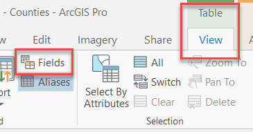
- Go to the Table > View tab and select Fields by unchecking the highlighted fields below and click Save.
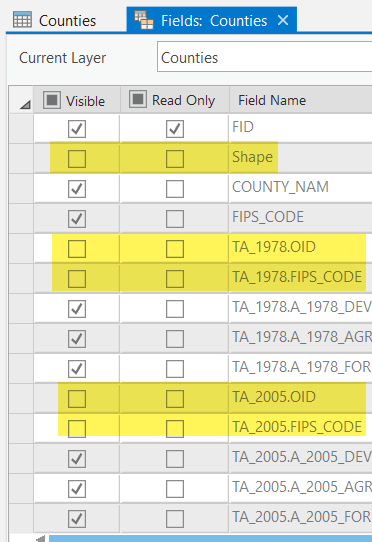
- Close the Counties attribute table if it is open and then open the attribute table again to see the results.
Make sure you have the correct answer before moving on to the next step.
Your attribute tables should match the examples below. If your data does not match this, go back and redo the previous step.
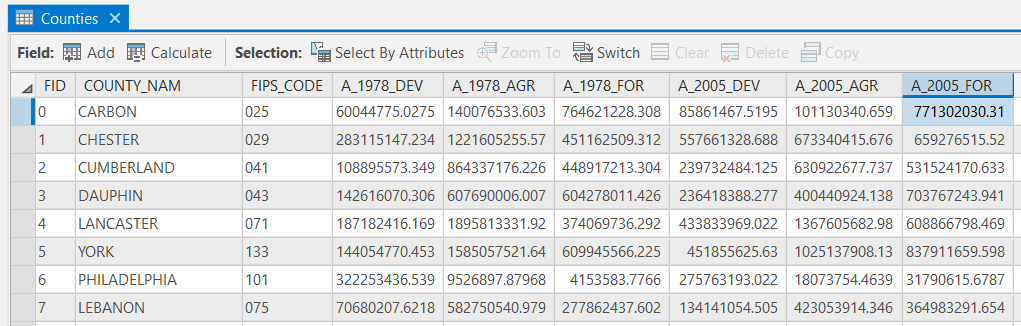 Click for a text alternative to the image above.
Sample Data, Counties FID county_Nam FIPS_code A_1978_Dev A_1978_agr A_1978_for A_2005_Dev A_2005_agr A_2005_for 0 Carbon 025 60044775.027 140076533.603 764621228.308
85861467.5195 101130340.659
771302030.31 1 Chester 029 283115147.23 1221605255.57 451162509.312 557661328.68 673340415.676
659276515.52 2 Cumberland 041 108895573.349 864337176.226
448917213.304 239732484.125 630927677.737 531524170.633 3 Dauphin 043 142616070.306 607690006.007 604278011.426 236418388.277 400440924.138 703767243.941 4 Lancaster 071 187182416.169 1895813331.92 374069736.292 433833969.022 1367605682.98 608866798.469
5 York 133 144054770.453 1585057521.64
609945566.225
451855625.63 1025137908.13
837911659.598 6 Philadelphia 101 322253436.539 9576897.87968 4153583.7766 275763193.022 18073754.4639 31790615.6787 7 Lebanon 075 70680207.6218 582750540.97 277862437.60 134141054.505 423053914.346 364983291.654 - Right-click on the "Counties" shapefile and choose Data > Export Features. Be sure to export all records and name it "LU_Change" in your L5 folder. Select "Yes" to add the shapefile to your map. Review the results.
- Right-click on the "Counties" shapefile and choose Joins and Relates > Remove Joins > Remove All Joins.
- Save your project.
- Right-click on the "Counties" shapefile and choose Joins and Relates > Add Join. Use the settings below and click "Validate" and then "OK". There may be a warning about the .dbf file not being indexed, it is OK to proceed.
-
Calculate the Area of Each County
- To identify the percent change over time for the three land-use layers, we first need to calculate the area of each county. Open the "LU_Change" attribute table and add a new float field called "TotAreaSQM" and Save. We need to use a float type since our numbers exceed the limits for short and long integers.
- Close the "LU_Change" attribute table.
- Reopen the "LU_Change" attribute table and populate the "TotAreaSqm" field using the "Calculate Geometry" tool. Make sure you use units of square meters.
Sometimes your calculated values will have too many digits to be stored in a long integer field. In these situations, you can use a data type of "float" instead.
-
Calculate the Percent Change Over Time By County and Time Period
As we saw in Lesson 2, it is much easier to compare numbers using percent areas vs. calculated areas. In this step, we are going to calculate the percent change within each land use type between 1978 and 2005.
- Before we can complete the calculations, we need to add new fields to hold the results. Add three new short integer fields using the names below.
- PctChg_dev
- PctChg_agr
- PctChg_for
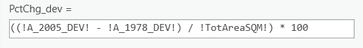
- We are going to use a semi-complicated equation to avoid the extra steps of calculating the percent area of each category, in addition to calculating the percent change over time. The basic equation we will use is:
Note: Although you can represent a percentage as a fraction, multiplying that fraction by 100 will give you a range of 0 to 100%.
([ tot land use in later time] - [ tot land use in earlier time]) / [TotAreaSqm]) * 100
- Calculate the percent change for each of the three new fields using the equation above. For example, to calculate the field "PctChg_dev," the equation would be:
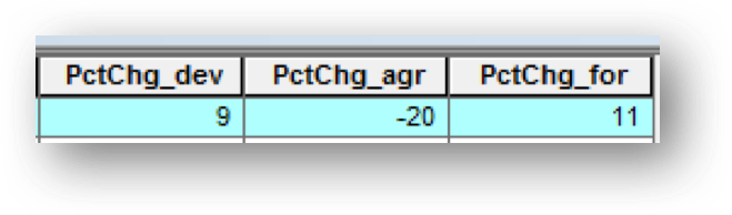
Make sure you have the correct answer before moving on to the next step.
Your calculated values should match the example below. If your data does not match this, go back and redo the previous step. I have only included the values for Adams County. You may need to sort your results to find this county.
- Before we can complete the calculations, we need to add new fields to hold the results. Add three new short integer fields using the names below.
-
Visualize Your Results Using Maps
Create a map layout with the 4 map frames below. (Note: You will not turn in these maps. However, you will need to consult them to complete the Lesson 5 Quiz).
- One data frame showing the agricultural land cover change between 1978 - 2005.
- One data frame showing developed land cover change between 1978 - 2005.
- One data frame showing forest land cover change between 1978 - 2005.
- One data frame with a locator map.
- Label each county with the % land cover change.
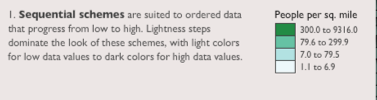
- Select a consistent color scheme that allows you to compare the three maps (e.g., red = increase, green = decrease, gray = no change)
In Lesson 5, we used the Reclassify Tool to collapse complex categories into simpler versions. We also used it to eliminate portions of our starting data that we did not need for our analysis using the "NoData" code. Can you think of any other ways you could use this tool?
That’s it for the required portion of the Lesson 5 Step-by-Step Activity. Please consult the Lesson Checklist for instructions on what to do next.
Try This!
Try one or more of the optional activities listed below.
- Use the Color Brewer website to help you choose symbology that highlights trends and spatial patterns in your data.
- Use the USDA/NRCS Geospatial Data Gateway Site to download land use data for an area of interest. Try reclassifying the data using the standardized categories from this lesson.
- Download the municipal boundaries for Pennsylvania using the PASDA site. On the home page, click on the “Boundaries” shortcut and select "Pennsylvania municipality boundaries." Use this file to define your zones instead of the county boundaries.