Part III: Identify the Potential Suitable Sites for Sludge Disposal

Part III: Identify the Potential Suitable Sites for Sludge Disposal

Now that the groundwater vulnerability layer has been produced, we can use this data to help find the areas in the watershed most suitable for sludge disposal. Along with this dataset, we also need to incorporate the stream buffer dataset. Remember from previous lessons that it is possible to reclassify grid cells to values of "NoData" to exclude them from your analysis. We will use this technique to remove portions of each dataset that do not meet the relevant criteria. For example, we will reclassify suitable areas within each dataset as "1" and unsuitable areas as "NoData."

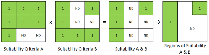
You can also do the opposite of this by assigning existing values of "NoData" to more meaningful values. We will use this technique to create a grid of areas that are outside of steam buffers. Then, we will use the Raster Calculator to combine the individual suitability results into one grid. We will then use the "RegionGroup” command to create regions from adjacent cells with the same results. This process is illustrated in the graphic below.

1. Explore the DRASTIC Rating Output Grids

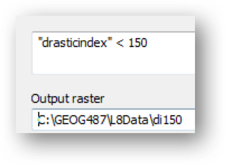
   1. In Part II Step 3, we talked about the potential pitfalls of using the reclassify tool when break values are important in your results. One way to avoid this issue is to use the Raster Calculator, which allows us to use mathematical sign of less than or greater than. Enter the expression shown below and name your grid "di150."
      
      

      The calculation performed in the previous step combines the results of two Boolean operations that are either evaluated as:

      TRUE (indicated by a value of 1) OR 
FALSE (indicated by a value of 0)

      We are only interested in cells that meet the criteria (values of 1).

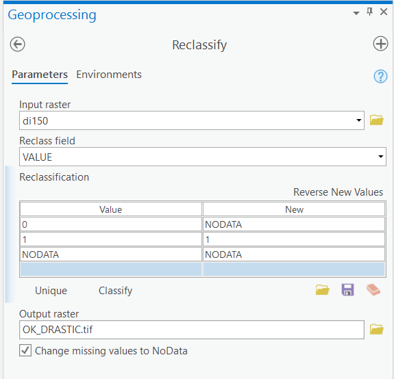
   2. Reclassify the "di150" grid using the settings below. Name the output grid "OK_Drastic.tif" and confirm the tool Environments.
       
      
      

      Make sure you have the correct answer before moving on to the next step.

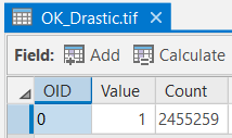
      The "OK_DRASTIC.tif" attribute table should have all of the attributes shown below. If your data does not match this, go back and redo the previous step.

          
       

2. Create a Grid of Suitable Surface Water

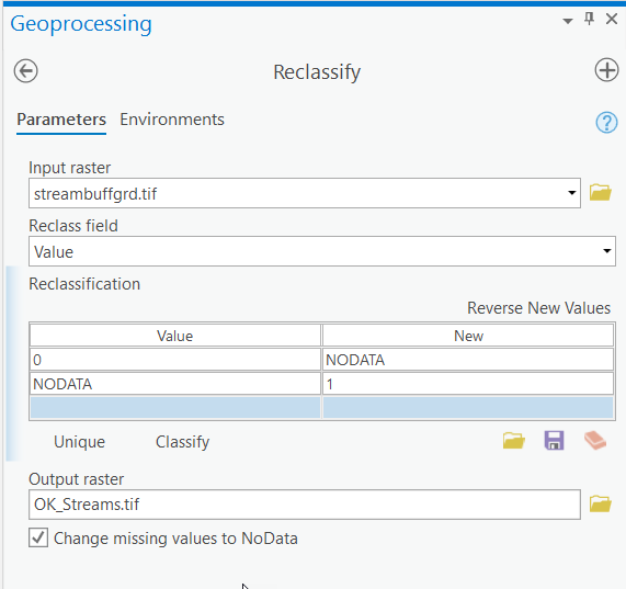
   1. Convert the "steams_buffer" shapefile to a raster using the "Id" field. Name the output "streambuffgrd.tif" and save it in your L8 folder and confirm the tool Environments.
   2. Reclassify "streambuffgrd.tif" as shown below. Name the output "OK_Streams.tif" and confirm the tool Environments.
      
      

      Make sure you have the correct answer before moving on to the next step.

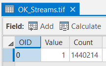
      The "OK_Streams" attribute table should have all of the attributes shown below. If your data does not match this, go back and redo the previous step.

       
   3. Compare the "OK_Streams.tif" layer to the "steambuffgrd." Notice how we have essentially flipped the areas of NoData. It is important that you choose an appropriate mask and extent settings when using this technique.

3. Combine the Suitability Grids Using the Raster Calculator

   1. Use the raster calculator to multiply the "OK_Drastic.tif" and "OK_Streams.tif" rasters together. Cells that meet both of the criteria will be assigned a value of "1" in the output raster. Cells that do not meet either one or both of the criteria will be assigned a value of "NoData" in the output raster. Name the new grid "OK2criteria."
      

      Make sure you have the correct answer before moving on to the next step.

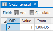
      The "OK2criteria.tif" attribute table should have all of the attributes shown below. If your data does not match this, go back and redo the previous step.

      
   2. Examine the attribute table. Notice there is only 1 row. We need a way to lump together cells that make up contiguous units. To accomplish this, we will use the Region Group tool like we did in Lesson 7.
   3. Go to Toolboxes > Spatial Analyst Tools > Generalization > Region Group, select " OK2criteria.tif" as the input raster, name the output raster " OK_Regions ", leave the number of neighbors to use as "FOUR", the zone grouping method as "WITHIN", uncheck the "Add link field to output", leave the excluded value setting , and click OK.
      

      Make sure you have the correct answer before moving on to the next step.

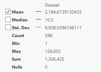
      The "OK_Regions" statistics for the "COUNT" field should match the example below. If your data does not match this, go back and redo the previous step.

      
           

4. Create Grid of Suitable Regions Greater than 0.5 sq km

   1. The last criteria we need to incorporate is - Area (sites greater than 0.5 sq km). We learned in Lesson 5 that you can calculate the area of a raster by multiplying the number of cells by the area of each cell. To calculate the area of regions within a raster, we can use this same method.

   2. Add a new float field to the "OK_Regions" attribute table named "AREA_SQM." Use the field calculator to populate the field.
      
      

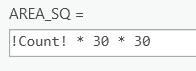
      Why did we use the number "30" to calculate the area?
      
      
      
       

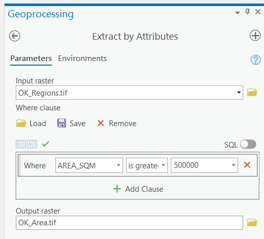
   3. We will use Extract by Attributes to perform a query on sites > 0.5 sq km. Extract by Attributes is similar to the Raster Calculator, except that it makes entering specific field expressions much easier.
   4. Go to Toolboxes > Spatial Analyst Tools > Extraction > ExtractByAttributes. Select "OK_Regions.tif" as the input raster and name the output raster "OK_Area". To populate the "Where clause" with the expression given below, click the "Query Builder" button. The "Query Builder" dialog will appear. Click on "AREA_SQM", and then on "greater than or equal to", and type 500000 at the end of the expression (0.5 sq km = 500,000 sq m). Confirm the tool Environments. Click Run to automatically input the expression into the "Where clause."
      
      

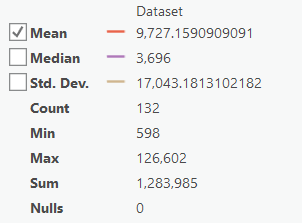
      Make sure you have the correct answer before moving on to the next step.

      The "OK_Area" statistics for the "COUNT" field should match the example below. If your data does not match this, go back and redo the previous step.

          
       
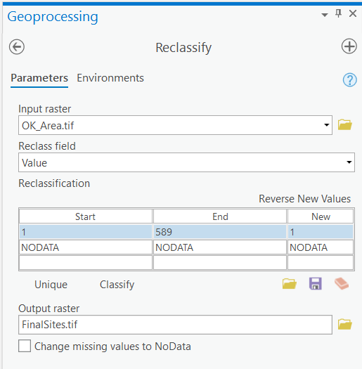
   5. Reclassify "OK_Area.tif". Change the number of classes to "1," since all of the start and end values match all of the site selection criteria. Name the grid "FinalSites.tif" and confirm the tool Environments. These are your potential sludge disposal sites.
      
          
      This is all for the required portion of the Lesson 8 Step-by-Step Activity. Please consult the Lesson Checklist for instructions on what to do next.