Step-by-Step Activity
Step-by-Step Activity: Overview
Step-by-Step Activity: Overview
The Step-by-Step Activity for Lesson 3 is divided into two parts. In Part I, we will look at publicly available datasets from Esri, the Fish & Wildlife Service National Wetlands Inventory, the Great Lakes Coastal Wetlands Inventory, and aerial photos from the USDA Farm Service Agency. In Part II, we will explore site-level data from three time periods that was digitized from high-resolution aerial photos. We will use the various datasets listed above to practice many of the data customization tasks covered in the lesson text.
Lesson 3 Step-by-Step Activity Download
Note: You should not complete this step until you have read through all of the pages in Lesson 3. See the Lesson 3 Checklist for further information.
Part I: Explore Publicly Available Wetlands Data & Historical Imagery
Part I: Explore Publicly Available Wetlands Data & Historical Imagery
Part I, we will explore our study area and the time-series aerial photos used to digitize the vegetation data we will use in Part II. We will also look at two publicly available datasets specifically related to wetlands: the National Wetlands Inventory from the U.S. Fish & Wildlife Service and a more detailed wetlands inventory from a regional public agency called the Great Lakes Commission. In the process, we will explore several different data delivery options and sources in ArcGIS: Esri Map Packages, Esri Basemaps, ArcGIS Online Datasets, Web Map Services (WMS) from GIS Servers, and raw GIS files.
-
Familiarize Yourself with the Study Area and Set Up Your Map
- Open the L3_Data folder you downloaded in the Lesson Data section. Double-click on the “Lesson3.mpkx” map package file. Designate your L3_Data folder as the unpacking location. This will open a map inside ArcGIS Pro with the study area boundary and historical imagery already loaded.

You can share your own data and maps by creating a map package in ArcGIS Pro. Go to the Share tab, Package group, and select Map Package
 . The file can either be uploaded to ArcGIS Online or saved locally.
 - Set your Current Workspace and Scratch Workspace to your L3 folder by navigating to the Analysis tab, Geoprocessing group, Environments
 . Make sure to read the associated help topics about “Current Workspace” and “Scratch Workspace.”
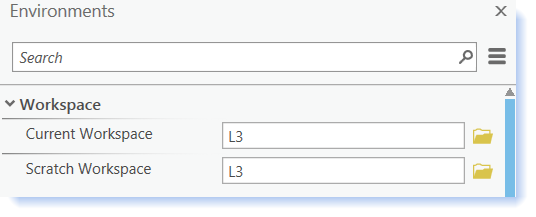
Setting your Current Workspace allows you to customize the location of where output files created during geoprocessing steps are saved. By default, files will be saved at …My Documents\ArcGIS.
To easily access information related to geoprocessing parameters and environments in ArcGIS: Click on the information icon
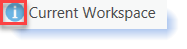 which will open a dialog window with information about usage and options. It is also a good idea to read the help information related to tools you are not familiar with (click
  or go to the Project tab > Help).
 - Add the “Open Street Map” ArcGIS Online Service (go to the Map tab, Layer group, click on Basemap
 > select OpenStreetMap) so you can tell where the study area is located in relation to the other places. You may need to refresh your map for the Basemap to load. (You need to be connected to the Internet and Signed In to the PSU AGO Organization using your WebAccess account information).
- Use the Explore tool
 found on the Map tab, in the Navigate group to take a look at the study site and the surrounding area. What is the nearest major city? How far away is the site from the state border with Michigan?
 - Turn off the Basemap, as this can slow down the drawing speed of your map in late steps. Save your project.
- Open the L3_Data folder you downloaded in the Lesson Data section. Double-click on the “Lesson3.mpkx” map package file. Designate your L3_Data folder as the unpacking location. This will open a map inside ArcGIS Pro with the study area boundary and historical imagery already loaded.
-
Explore Historical and Recent Aerial Photos
- Zoom to the study area boundary by right-clicking on it in the Contents pane > Zoom to Layer.
- Turn on the “2005” layer in the Contents pane. This is a Color Infrared (CIR) image. Notice the information on the edge of the scanned film showing the date, location, and scale of the original image.
- Turn on the “1973” and “1962” images. These images are black and white, a common format before 2000.
- Compare the three images by turning them on and off and viewing them at a number of different scales: 1:15,000, 1:10,000, and 1:5,000. Try navigating to different locations within the study area. What differences do you notice between the three images?
Take a minute to look at the swipe and flicker tools available on the Raster Layer, Appearance tab, Compare group (be sure an image is highlighted in the Contents pane) These tools can be useful for temporal change detection (especially of satellite images or air photographs that were taken at different times of the same location), data quality comparison, and other scenarios where you want to visually compare the differences between two layers in your map. Swipe allows you to interactively reveal what is underneath a particular layer; Flicker flashes layers on and off at the rate you specify. You can read more about these tools in Esri help.
- The photos that were used to create the detailed vegetation data we will use in Part II all show the study area in the past. Let’s take a look at more current imagery and see if we notice any changes in the vegetation. We’ll use an image from 2018 to 2020 from the National Agricultural Imagery Program (NAIP).
- We can add ArcGIS Online data to the Map by going to the Map tab, Layer group, Add Data > Data. Under Portal, click ArcGIS Online.
- Search for USA NAIP Imagery. Click OK.
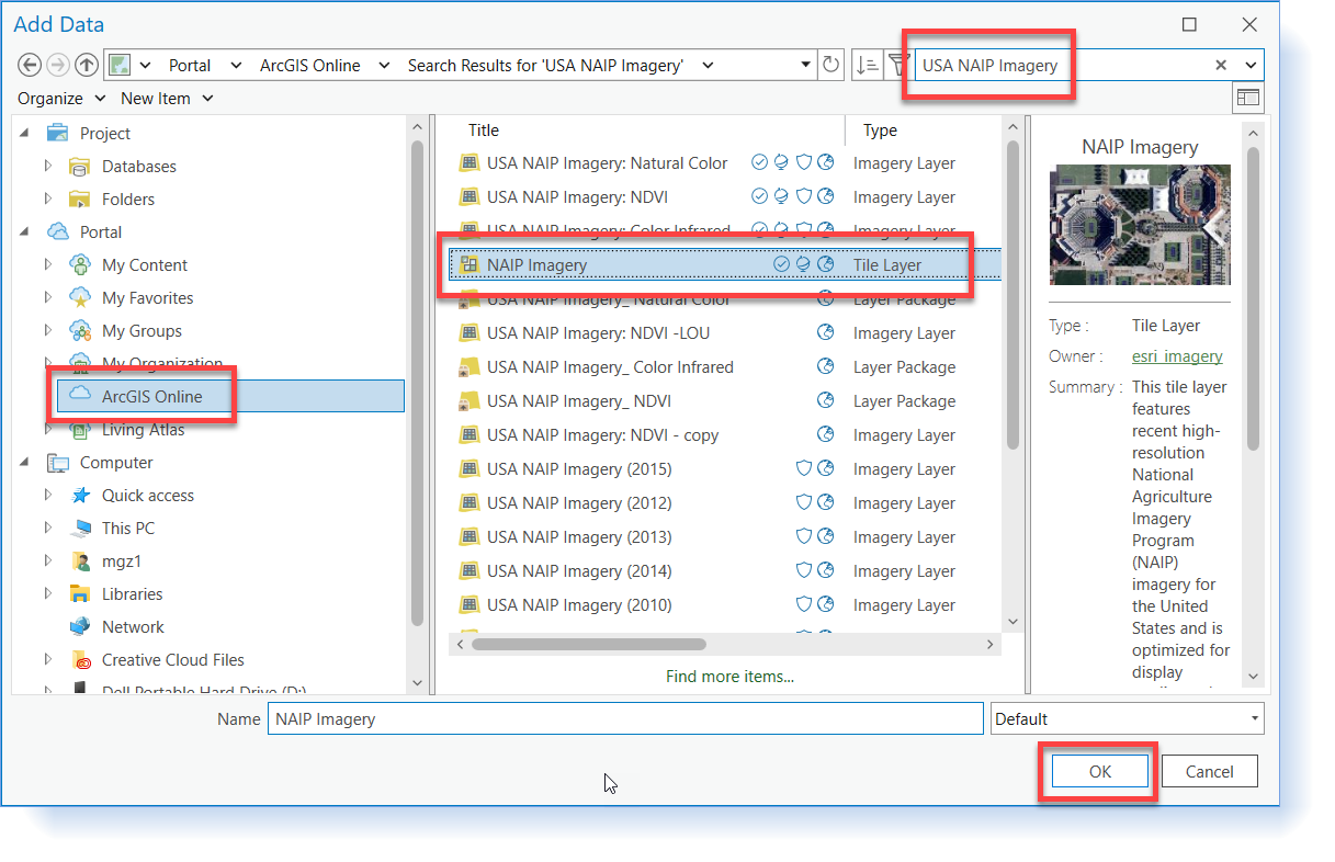
- The USA NAIP Imagery layer will be added to the Contents pane.
- Compare the NAIP Imagery with the historical aerials. What types of changes do you see? Notice that the NAIP Imagery is more natural in color, which is a bit easier to interpret (as compared to color infrared and black-and-white formats).
- Turn off the imagery layers in the Contents pane and save your project.
-
Add the boundaries of the Fish & Wildlife Service Wildlife Refuges to your map
- Again go to the Map tab, Layer group, Add Data > Data. Under Portal, click ArcGIS Online.
- In the ArcGIS Online search window, type “national wildlife refuges” Review the datasets that match the search. Locate the "National Wildlife Refuges” dataset in the results.
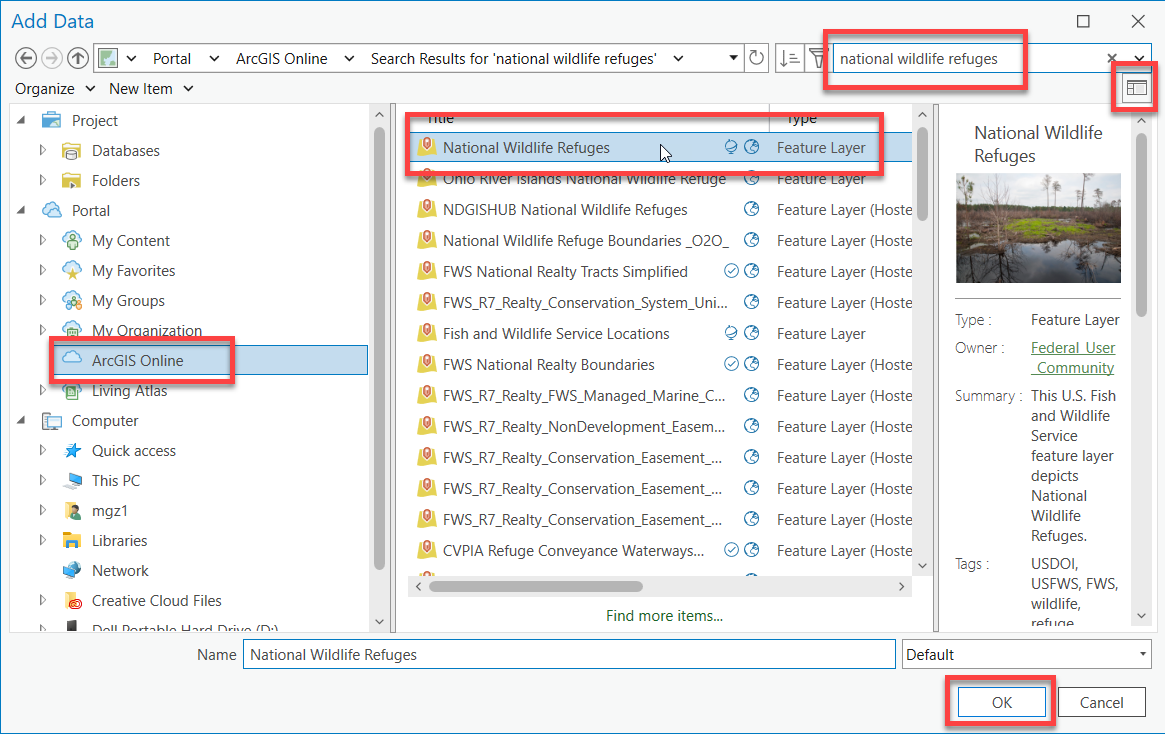
- Click on the "Details" button to review the metadata. Notice that this data is a Feature Layer and was last modified on 7/25/2022. Click OK to add the layer to the Map.
- Drag the study site boundary to the top of the Contents pane so you can see the site boundary on top of the feature service.
- Zoom out to 1:250,000 so that you can see the various federal lands in the vicinity. The refuge is shown as a pinkish-filled polygon, which means it is a Great Lakes National Wildlife Refuge. Use the explore tool to click on the feature and identify the refuge's name.
- Notice how the lesson study area only covers a portion of the whole refuge. The study site boundary represents the wetland areas within Ottawa National Wildlife Refuge that are hydraulically connected to Lake Erie. Some of the wetlands in the refuge are excluded from this area because they are hydraulically separated from Lake Erie by dikes and are therefore not susceptible to fluctuations in Lake Erie water levels. Other areas of the refuge are not wetlands.
- Right-click on the “FWSBoundaries” layer name in the Contents pane > select Attribute table. Explore the attribute table. Are there any abbreviations you don’t understand?
- Again, right-click on the “FWSBoundaries” layer > Properties > Source > Spatial Reference. Look at the spatial reference information. Is it the same as the study site? Does it match the data frame? (Right-click on StudyArea in the Contents pane > Properties > Coordinate Systems). Note: You may experience errors editing a data layer if it does not match that of the data frame.
-
Create a new shapefile of the Ottawa National Wildlife Refuge Boundary
- Right now, the refuge boundaries on our map are part of a feature layer. We want to create a new shapefile from just a portion of the records so we can customize it for our study site.
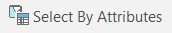
- Open the FWSBoundaries attribute table. Click on the “Select by Attributes” icon
 .
. - Create a new selection expression to select all of the polygons within the Ottawa National Wildlife Refuge Where "Organization Name" is equal to "Ottawa National Wildlife Refuge". Apply the expression. You should have 1 of 574 records selected. Close the attribute table. Notice that the polygon is a multipart feature, or it has more than one part but is defined as one feature because it references one set of attributes. Confirm this by viewing the attribute table.
- Right-click on the layer in the Contents pane and click Data > Export Features. Export the selected features to a new shapefile called “OttawaNWR.shp” to your L3 folder. Make sure to go to the Environments tab in the Export Features dialog to establish the Output Coordinates as the same coordinate system as the Current Map [Study Area], or you may not be able to edit this data later on in the lesson.
- The “OttawaNWR” shapefile will be added to your map. Verify the Coordinate System (Properties > Source > Spatial Reference) is the same as the StudyArea Map. Remove the “FWSBoudaries” dataset from your map and save the project.
- Save your project.
-
Download and Explore the National Wetlands Inventory (NWI) Data
- Connect to the National Wetlands Inventory data service. Go to the Insert tab, Project group, and click on Connections > Server > New WMS Server > Copy and paste the URL: https://www.fws.gov/wetlandsmapservice/services/Wetlands/MapServer/WMSServer? [1] and click OK.
- Go to the Map tab, Layer group, Add Data > Data. (Note: If you cannot view the layer using Add Data, try dragging the wetland layer from the Catalog pane > Project > Servers to the Map).
- Under the Project folder, click on Servers. Double-click on WMS (www.fws.gov.wms [2]) > WMS > Layers. Highlight the Wetlands layer and click OK to add the data set to your map. The layer will be added to the Contents pane and will be named WMS > Wetlands.
- Drag the WMS Wetlands layer toward the top of the Contents pane but under the Study_Site layer. Zoom to the study area layer and explore the data.
- Use the Explore tool from the Map tab to see what information is included with the layer. Notice that you can’t view an attribute table like you could with the feature layers.
- According to the metadata [3], “the data are intended for use with base maps and digital aerial photography at a scale of 1:12,000 or smaller. Due to the scale, the primary intended use is for regional and watershed data display and analysis, rather than specific project data analysis.”
- Unfortunately, the data does not contain enough detail to help us analyze vegetation changes in a specific wetland. It also does not allow us to study changes over time.
- Turn off the “WMS” layer in the Contents pane and save your project.
-
Explore the Great Lakes Coastal Wetland Inventory Data
- Read a quick description of the data at Great Lakes Commission [4] (scroll down to the "Links to Inventory and Metadata" heading). Notice the link to the product metadata provided on the site. We are going to use one file from this site called, “the complete polygon coverage in shapefile format.”
- Download the data zip file from the site or from the Lesson Data page (glcwc_cwi_polygons.zip [5] - 12.46 MB), save it in your L3 folder, and unzip the file.
- Add the “glcwc_cwi_polygon” shapefile to your map.
- Open the attribute table and explore the available information. Notice how there is significantly more information than the previous wetland datasets we reviewed.
- The “HGM_CLS1” and “HGM_CLS2” attributes show the wetland classification codes. You can read detailed descriptions of these codes in the “Great Lakes Coastal Wetlands [6]" (enhanced metadata) document.
- Right-click on the “glcwc_cwi_polygon” shapefile in the Contents pane > Zoom to Layer. It is difficult to see any detail.
- Zoom back to the Study_Site layer. Do you see any wetlands inside the Ottawa National Wildlife Refuge that are not inside our study site boundary? You may need to move the Study_Site boundary layer and OttawaNWR layers to the top of your Contents pane.
- Turn the layer off in your Contents pane and save your project.
- The Great Lakes Coastal Wetland Inventory provides much more detailed attribute information than the National Wetlands Inventory. However, it still doesn’t provide the time-series information we need to answer our research questions. For time-series data, we need to look at yet another data set.
Part II: Explore & Customize Site Level, Time Series Wetlands Data
Part II: Explore & Customize Site Level, Time Series Wetlands Data
The publicly available datasets we just explored are helpful for familiarizing yourself with your study area or for regional or other large-scale analyses. However, they do not contain the level of detail for the site level analysis we want to conduct. The highest resolution data you can usually find is 1:24,000 scale for vector data and 30 m cell size for raster data. Publicly available datasets also typically do not have time-series information available. In Part II, we are going to explore a high resolution, time-series dataset that was digitized from the aerial photos we reviewed in Part I. Oftentimes, you will need to digitize information in this manner if you have a small study site or if you want to do an in-depth, time series analysis. The work required to create the data is significant. However, you can do a lot more with your data.
We want to explore how vegetation has changed over time in our study area. To answer our research questions, we need the following datasets: 1) polygons of vegetation species over time 2) polygons of vegetation groups over time, and 3) polygons of invasive species over time. All of the files need to show just the region within our study site. We will create these custom datasets for three time periods using the Join, Union, Clip, and Dissolve tools. The workflow we will follow is illustrated in the diagram below using the data for the seventies time period. You may wish to consult this diagram after completing each step.
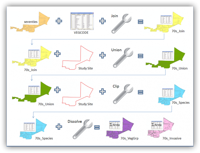
- Seventies + VEGCODE + join = 70s_Join
- 70s_Join + Study Site + union = 70s_union
- 70s_union + Study Site + clip = 70s_species
- 70s_species + dissolve = 70s_VegGrp + 70s_Invasive
-
Explore the Site Level Vegetation Data
- Open the map from Part I.
- Add the “sixties,” “seventies,” and “twothousands” vegetation shapefiles from the L3 folder to your map.
- The default symbology should show the vegetation polygons filled in. Do you see any gaps in coverage between the vegetation data and site boundary? Hint: turn some of the layers on and off and use the zoom tools. Look along the coastline along the northeast boundary.
- Compare the extents of the vegetation data and study site. Do you see any differences?
- Open the attribute tables. Do you notice any differences in the number of records in each dataset? Do you see any coded or missing values? Missing data may sometimes be coded as values of “0.”
- Notice how the vegetation files contain a lot more spatial detail than the publicly available datasets we looked at earlier. At this point, we do not know what the values in “VEG_ID” mean, though we can assume they correspond to different types of vegetation. Even without knowing what the “VEG_ID’s” mean, we can still tell that the "twothousands" data has a lot more polygons than the other time periods. What do you think the VEG_ID code “11” means?
-
Understand Coded Values
- Now that we have a general sense of what our starting data looks like, we can work on customizing it for our purposes. Let’s start by figuring out what the coded values in the “VEG_ID” fields mean.
- Add the “VEGCODE.dbf” table from your L3 folder to your map. Open the table.
- The VEGCODE table is a master lookup table that tells us what the coded values (VEG_IDs) mean. The VEG_IDs correspond with detailed vegetation types (Veg_Type).
- I have reclassified this information for you into 2 simpler categories: Veg_Group and Invasive. The numbers at the beginning allow us to sort the values based on the depth of water they prefer (e.g., most water (open water) to least water (upland vegetation) instead of alphabetically by name).
Note: You may notice that some of the Veg_IDs are listed as “May Be Invasive” in the “Invasive” field. Two of the most common invasive species in the wetland (narrow-leaved and hybrid narrow/broad-leaved cattails) look very similar to native species (broad-leaved cattails,) which makes them difficult to distinguish in aerial photos.
- Join the VEGCODE table to the sixties vegetation shapefile Right-click on the “sixties” shapefile > Joins and Relates > Add Join. Base the join on the Veg_IDs. Keep All Target Features. Validate the join and then click OK.
Caution - watch out for similar attribute names like OID. This is not the same as Veg_ID.
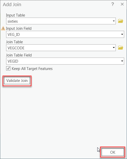 Add Join
 - Open the attribute table of the sixties shapefile to make sure the join worked properly.
- To make the join permanent, export features to a new shapefile in your L3 folder called “60s_Join.” Be sure the new shapefile is added to your map.
- Repeat steps e - g for the remaining two vegetation data sets. Name them “70s_Join” and “00s_Join.” Remove the “sixties,” “seventies,” “twothousands,” and VEGCODE table from your map and save.

Make sure you have the correct answer before moving on to the next step.
The 60s_Join, 70s_Join, and 00s_Join shapefiles should have the number of records and all of the attributes shown below. If your data does not match this, go back and redo the previous step.
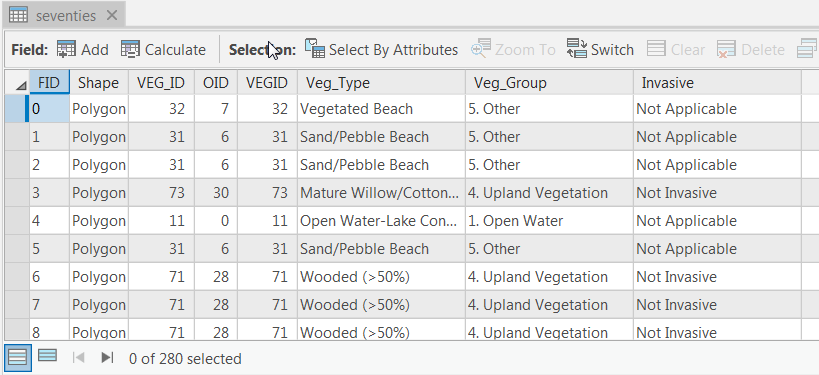 60s_Join - 352, 70s_Join – 280 records and 00s_Join – 449 records.
 -
Modify Extents - Fill in Gaps
- We want all of our input data sets to have the same total area so we can compare changes in the area of different vegetation types over time. This means we need to remove pieces from some study years and fill in gaps for other years so they all cover the same extent.
- First, we will fill in gaps. A quick way to fill in gaps is to use the union tool to create new polygons in areas that overlap within the extent of two datasets. We will union the vegetation shapefiles with the study boundary since this file does not have any gaps and it covers the area we are interested in. Follow the steps below to union the two files:
- Go to the Analysis tab, Tools group > Union
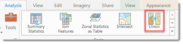 Union tool.
 - Click on the “Show Help” button for more information about what the tool does and what the different input criterion means.
- Input Features: Study Site; 60s_Join (make sure the study site is listed first).
- Output Feature Class: 60s_Union.shp (save it in your L3 folder not in the default.gdb).
- Keep the defaults for Join Attributes (ALL).
- Make sure the “Gaps Allowed” checkbox is NOT checked. Read the help topic about this, so you understand why.
- Keep the defaults for the Environments.
- Click Run.
- Compare the output file to the original shapefile from the same time period to make sure the tool worked as expected. Notice the records that have an FID_Study_ value of -1. What do these mean? Hint: See step vi.
- Repeat union for the remaining two vegetation shapefiles “70s_Join” and “00s_Join.” Name them “70s_Union” and “00s_Union.”
Geodatabases may have naming restrictions for table and field names. For instance, a table in a file geodatabase cannot start with a number or a special character such as an asterisk (*) or percent sign (%). Shapefiles do not have such restrictions and allow us to use names such as 60s_Join.
If you receive an Error 000361: The name starts with an invalid character during geoprocessing, check to make sure you are saving your output as a shapefile.
It’s very easy to make mistakes when using geoprocessing tools. For example, you can select the wrong input files by mistake. Another common error is running tools while unknowingly having records selected. Any output from geoprocessing tools will only contain the selected records. Comparing your results with your input datasets after using automated tools is a good habitat to get into.
If you want to double-check the input files you used previously, the parameter settings, environment settings, etc., you can view them under Geoprocessing > History.
Make sure you have the correct answer before moving on to the next step.
- 60s_Union should have 367 records
- 70s_Union should have 289 records
- 00s_Union should have 458 records
If your data does not match this, go back and redo the previous step.
-
Modify Extents - Remove Excess Area
- Notice that some of the study years still cover a larger area than others. For example, compare the 60s_Union shapefile with the 70s_Union shapefile. Let’s change the extent of all data sources to match the study area boundary by using the clip tool. Note: The Clip tool is only for vector datasets. In later lessons, we will look at tools to clip raster datasets.
- Go to the Analysis tab, Tools group > Clip

- Click on the “Show Help” button for more information about what the tool does and what the different input criteria mean.
- Input Features: 60s_Union.
- Clip Features: Study_Site.
- Output Feature Class: 60s_Species.shp (save it in your L3 folder).
- Keep the defaults for Environments.
- Click Run.
- Go to the Analysis tab, Tools group > Clip
- Compare the output file to the joined shapefile and unioned shapefile from the same time period. What differences do you notice?
- Clip 70s_Union and 00s_Union using the directions above. Name them “70s_Species” and “00s_Species.”
Make sure you have the correct answer before moving on to the next step.
- 60s_Species should have 240 records
- 70s_Species should have 206 records
- 00s_Species should have 325 records
If your data does not match this, go back and redo the previous step.
- Remove the original vegetation, unioned, and joined shapefiles from your map and save the project.
- All of our study years should now have the same extent. Let’s confirm this by calculating the area of each study year. Add a new double field
 to each year called “sqm” with the default scale and precision values. I find it helpful to name fields by their units so I remember what they mean later on. Remember to
  your changes.
Specifying a specific precision and scale when adding a field to a shapefile gives you the option to limit the number of digits (precision) and decimal places (scale) of values within number fields. There are many situations where you would want to do this. However, there are also occasions where it is best to keep all of your options open. Accepting the default value of 0 for both properties gives you the most versatility. It may seem counterintuitive, but the value of 0 acts somewhat similar to the value of infinity in this case. Setting custom precision and scale values is only relevant to data stored in an enterprise geodatabase. Default values are always enforced when editing data in a shapefile or file geodatabase. Refer to the ArcGIS field data types [7] for more information.
I recommend using values of 0 when you are in the preliminary stages of data exploration. That way you won’t unknowingly exclude values in your results. For example, if you are calculating area values for the first time, you probably won’t know how many digits you will need to store your calculated values (precision) until after you’ve made the calculation. If you estimate a number to use for precision that ends up being too low, you will not be able to store the full range of values. For example, a precision of 2 would limit your values to two digits, whereas a precision of 4 would limit your values to four digits.
- In the open attribute table, right-click on the “sqm” field and click Calculate Geometry. Choose area and units of square meters. Use the coordinate system of the data source. Repeat this step for the remaining two shapefiles.
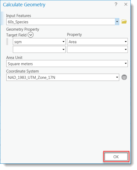 Calculate Geometry
 - Use the statistics tool to find the total area for each year by right-clicking on the “sqm” field and choosing “Statistics”. All of the study years should have the same “SUM” value. You may notice very small differences between the layers. This is due to tiny topology errors such as overlapping sliver polygons. We could have corrected these with the Environments > XY Tolerance settings during our union and clip operations if we needed this level of precision for our analysis. In this case, we don’t, but I wanted to point out this issue in case you come across it in other projects. For more information about XY Tolerance, see the Esri Help.
- Notice that some of the study years still cover a larger area than others. For example, compare the 60s_Union shapefile with the 70s_Union shapefile. Let’s change the extent of all data sources to match the study area boundary by using the clip tool. Note: The Clip tool is only for vector datasets. In later lessons, we will look at tools to clip raster datasets.
-
Explore Attributes & Missing Data
- Now that we’ve fixed the geometry of our input data, we can start to work with the attributes. Before inputting data into an analysis, you should have a good understanding of the distribution of your values. You should also be aware of any missing values or outliers that can skew your results, so you can exclude or recode these if necessary.
- One way to quickly get a sense of the distribution of data values and missing data is to change the symbology to be categorical based on each attribute.
- Right-click on the 60s_Species shapefile in the Contents pane > Symbology. The Symbology pane will open to the right. Under Primary symbology > Unique values > Field 1 Veg_Type.
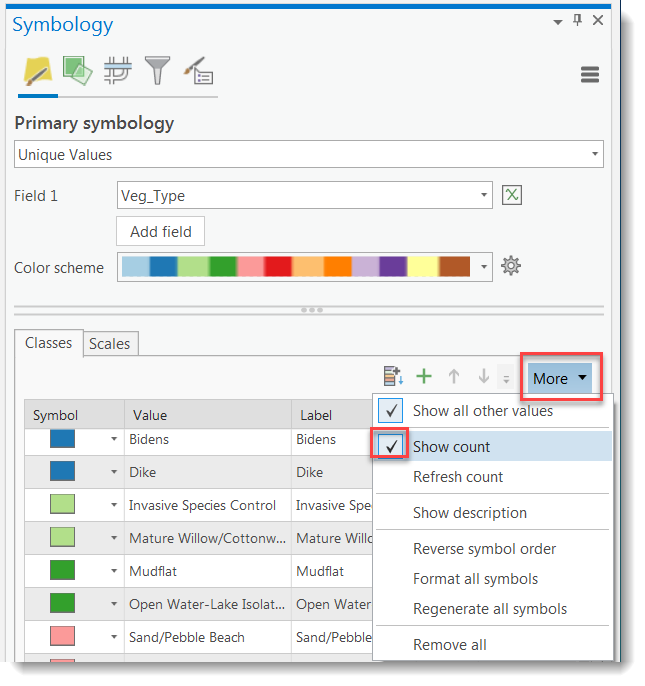 Symbology pane
 - Expand the More dropdown list and click on Show Count. How many polygons have missing data (blank entry) in the “Value” column? Do you see any values with typos?
- Repeat this process for the “Veg_Group” and “Invasive” variables.
- Repeat steps c and d for the remaining two time periods (“70s_Species” and “00s_Species”).
-
Generalize Data
- For our analysis, we are particularly interested in two attributes, “Veg_Group” and “Invasive.” Right now, each polygon represents vegetation clusters of the same species, which is more detailed than we need. We want to create two new data sets in which the polygons represent clusters of vegetation groups and clusters of invasive types over time. We will use these customized data sets in Lesson 4, where we will discuss how to interpret and present results from several datasets.
- First, let’s create the time series shapefiles of vegetation groups.
- Go to the Analysis tab, Geoprocessing group > Tools
 .
. - In the Geoprocessing pane, search for "Dissolve".
- Click on the “Show Help” button for more information about what the tool does and what the different input criteria mean.
- Input Features: 60s_Species.
- Output Feature Class: 60s_VegGrp.shp (save it in your L3 folder, not the default.gdb).
- Dissolve Field: Veg_Group.
- Statistics Field: Select “sqm” as the field and “SUM” as the statistics type.
- “Create multipart features” should be checked.
- “Unsplit lines” should NOT be checked.
- Go to the Analysis tab, Geoprocessing group > Tools
- Compare the output file to the input file from the same time period.
- Repeat the dissolve for the remaining two time periods. Name them “70s_VegGrp” and “00s_VegGrp.”
Summary Statistics tool (go to the Analysis tab, Geoprocessing group >Tools
> search "Summary_Statistics") is another option you can use to calculate statistics for your data. This tool is similar to the “Summarize” option available by right clicking on a field in an attribute table. The advantage of the Summary Statistics tool is that it allows you to create statistics based on multiple fields. For example, you could use it to find the total area for every unique combination of vegetation type and invasive classification. You could interpret the results to find out which plant type makes up the majority of invasive species for each time period.Multipart polygons are features that have more than one polygon for each row in the attribute table. If you want to explode these into individual records at a later time, there is a tool available on the Edit tab, in the Tools group.
- Now, let’s create the time series shapefiles by invasive type.
- Go to the Analysis tab, Geoprocessing group > Tools.
- In the Geoprocessing pane, search for "Dissolve".
- Input Features: 60s_Species.
- Output Feature Class: 60s_Invasive.shp (save it in your L3 folder).
- Dissolve Field: Invasive.
- Statistics Field: Select “sqm” as the field and “SUM” as the Statistics Type.
- “Create multipart features” should be checked.
- “Unsplit lines” should NOT be checked.
- Go to the Analysis tab, Geoprocessing group > Tools.
- Compare the output file to the input file from the same time period.
- Repeat step c for the remaining two time periods. Name the output files “70s_Invasive” and “00s_Invasive.”
- Remove the “60s_Species,” “70s_Species,” and “00s_Species” from your map and save.
That’s it for the required portion of the Lesson 3 Step-by-Step Activity. Please consult the Lesson Checklist for instructions on what to do next.

After experimenting with online data services in Lesson 2 and raw data in Lesson 3, which do you think is easier to work with? What are the pros and cons of each one? Can you think of any scenarios in which one is preferable over the over?
Do you have a good understanding of why we completed each step in Part II? If not, compare the starting vegetation files and final outputs (XX_Species, XX_VegGrp, XX_Invasive) in terms of extent, area, gaps, spatial detail, and attributes.
Try This!
- In Lesson 3, we familiarized ourselves with the study site using the “Open Street Map” layer from Esri. Google Earth Pro [8] is another excellent application for this purpose. If you are willing to install the software, try one or more of the activities listed below.
- Open the KMZ file of the Study Area (in the L3 Data folder) in Google Earth, zoom to the study boundary, and explore the area around the study site. For example, look for Street View images or other sources of imagery (Layers > More > DigitalGlobe Coverage). If you receive an error message by double-clicking directly on the KMZ file from Windows Explorer, open the file from within Google Earth > File > Open > Study_Boundary.kmz. You can also right-click on the KMZ file from your desktop > Opens With > Google Earth.
- Experiment with the “view historical imagery” tool by clicking on the clock icon to see if you can find these. How far back in time do the images go?

- Explore Great Lakes Phragmites Collaborative [9]. Can you find any other Phragmites projects along the Lake Erie shoreline?
Note: Try This! Activities are voluntary and are not graded, though I encourage you to complete the activity and share comments about your experience on the lesson discussion board.