Lesson 5: Land Use Change
Lesson 5 Overview and Checklist
Lesson 5 Overview and Checklist
Scenario
You have been hired by the Pennsylvania Department of Environmental Protection to determine how land cover has changed historically in southeastern Pennsylvania between 1978 and 2005. You know that land cover grid data is available for the time periods of interest, but the datasets are from two different sources. You also know that while each data set is similar, the land use/land change categories and codes do not match up perfectly between the different historical sources. You must use Spatial Analyst to help standardize all of the datasets and determine how much land area has changed over time by land cover category (agriculture, residential, etc.)
Goals
At the successful completion of Lesson 5, you will have:
- reclassified grid data using Spatial Analyst;
- tabulated areas using Spatial Analyst; and
- calculated change over time using tabular data.
 |
 |
 |
 |
 |
Questions?
If you have questions now or at any point during this lesson, please feel free to post them to the Lesson 5 Discussion.
Checklist
This lesson is worth 100 points and is one week in length. Please refer to the Course Calendar for specific time frames and due dates. To finish this lesson, you must complete the activities listed below. You may find it useful to print this page out first so that you can follow along with the directions. Simply click the arrow to navigate through the lesson and complete the activities in the order that they are displayed.
- Read all of the pages in Lesson 5.
Review the information on the "Background Information," "Required Readings, Video, and Podcasts" "Lesson Data," "Step-by-Step Activity," "Advanced Activities," and "Summary and Deliverables" pages. - Read, review, or listen to the required readings, video, and podcasts.
See the "Required Readings" page for links to the PDFs. - Download Lesson 5 datasets.
See the "Lesson Data" page. - Download and complete the Lesson 5 Step-by-Step Activity.
See the "Step-by-Step Activity" page for a link to a printable PDF of steps to follow. - Complete the Lesson 5 Advanced Activity.
See the "Advanced Activity" page. - Complete the Lesson 5 Quiz.
See the "Summary and Deliverables" page. - Optional - Check out additional resources.
See the "Additional Resources" page. This section includes links to several types of resources if you are interested in learning more about the GIS techniques or environmental topics covered in this lesson.
SDG image retrieved from the United Nations [1]
Background Information
Background Information
Land Cover Datasets
Land cover data represents continuous measurements from satellites such as Landsat, Sentinel, and MODIS. Raster products derived from satellite data, such as the National Land Cover Dataset (NLCD), are commonly used to study how much of a region is covered by forests, wetlands, impervious surfaces, agriculture, and other land and water types. We used an NLCD dataset updated in 2021 and created in 2019 in Lesson 2. NLCD is a national dataset with information on land cover for a given time period for all areas in the U.S. Each grid cell represents a particular land cover category and was derived from classification algorithms that processed Landsat satellite imagery. Currently, there are eight NLCD datasets [2] that represent 2001, 2004, 2006, 2008, 2011, 2013, 2016, 2019, and 2021 (2021 released in 2023). The NLCD is one of the most commonly used land cover datasets since it is available for such a large area and at multiple time periods.
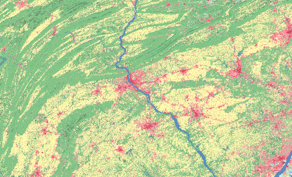
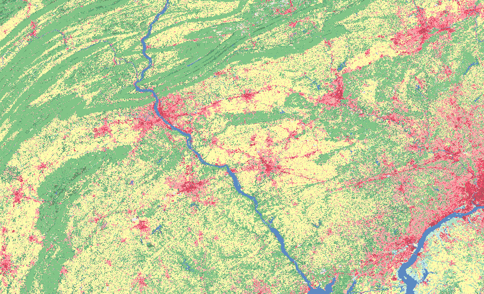
Land Cover Change - Urban Sprawl
Land cover change is a common issue that has a wide range of environmental implications. Land cover will be an important driver of climate change in the next century. Some reasons for this are the increase in impervious surfaces and the reduction of agricultural and forested areas, which reduce the uptake of CO2 by plants. By reviewing Figure 1, it is easy to see the effect of urban sprawl, even over just a fifteen-year period. The increased amount of red and pink cells (which represent developed area) you see in the 2016 data highlight the urban sprawl that is taking place. During urban sprawl, areas that were previously covered in forests, grasslands, wetlands, etc., have become developed areas.
The reduction of agricultural and forest land due to the spread of low-density, single-use development into rural areas can increase air and water pollution. The loss of these lands affects human health, biological stability, wildlife habitat, and long-term sustainability. The disappearance of agricultural lands can also impact food security by reducing the amount of available food for the immediate area. This will most likely drive up prices, which will affect the overall economic health of that area. Forest loss will reduce the habitat for native species, which will cause them to encroach in urban areas and possibly result in population reductions or even extinction in that area.
Required Readings, Video, and Podcasts
Required Readings, Podcasts and Video
The required readings for this lesson include a research project page, a journal article, a land cover and land use chapter, the NCLD fact sheet, a video, three USGS podcasts, and three Esri Help Articles. The land use change article highlights the importance of tracking land cover changes as they relate to various environmental issues. There are also three Esri articles related to operations we will use in ArcGIS during the Step-by-Step Activity. Although we will explain how to use these tools in the Step-by-Step text, the help topics will provide you with a good overview of what the tools will do when executed.
Land Cover Readings:
USGS Land Cover / Land Use Change Research [3]
Conterminous United States Land-Cover Change (1985–2016): New Insights from Annual Time Series [4] (Published: February 2022)
Fact Sheet: National Land Cover Database [5]
FOURTH NATIONAL CLIMATE ASSESSMENT Volume II: Impacts, Risks, and Adaptation in the United States:
Chapter 5, Land Cover and Land-Use Change [6]
Listen to USGS Eyes on Earth [7] Podcast Episodes:
JOHN HULT:
Hello everyone. Welcome to this episode of Eyes on Earth. We're a podcast that focuses on our ever-changing planet and on the people here at EROS and around the globe who use remote sensing to monitor and study the health of Earth.
My name is John Hult, and I will be your host for this episode.
If you are a regular listener, you have surely heard us talk about how the Landsat satellite data archive represents the longest continuously collected record of the Earth's surface in existence. You have also heard about how scientists monitor the health of the planet by looking back through that nearly 50-year record to track change. But how can data collected in 1972, by a satellite with 1972 technology, possibly align with data collected yesterday, by a satellite launched 40 years later? The answer, for the most part, is Collections. Landsat Collection 1 saw all that data calibrated to match up as closely as possible to match up as closely as possible across all 7 satellite systems. The work allowed scientists to track points on the surface of the Earth more easily and gave them more confidence in their conclusions.
The Landsat team at EROS has just released Collection 2. An upgrade that improves accuracy and expands access to higher level products like land surface temperature. Collection 2 also makes Landsat data available in a cloud friendly format.
Here with us to talk about Collection 2 is Dr. Chris Barnes a contractor at EROS who supports the Landsat International Cooperator Network. Dr. Barnes, thank you for joining us.
CHRIS BARNES:
Thank you very much. Great to be here.
HULT:
Also joining us is Dr. Christopher BARBER. A remote sensing scientist with the USGS Land Change Monitoring Assessment and Projecting Initiative also known as LCMAP. Dr. BARBER, thank you for joining us.
CHRIS BARBER:
Not a problem. Happy to contribute.
HULT:
Dr. Barnes and Dr. Barber, you both work in remote sensing. You are both names Chris. My guess is you have probably gone to the same conference once or twice. You guys must have had your luggage messed up at the airport at least once, right?
BARBER:
We have had frequent flyer miles mixed up.
HULT:
Oh really? Who was the beneficiary of that?
BARNES:
I'm pleased to say that it was me that took a trip to South America.
HULT:
Oh, nice. Let's get into Collection 2 here. Dr. Barnes, we are going to start with you. Why don't you tell us what the word "collections" means in relation to satellite data. How does a collection help scientists study the Earth?
BARNES:
Absolutely. That's a great question. Back in 2016, USGS released the first Collection, Landsat Collection 1, which was a major shift in the management of the USGS archive. Before that, the Landsat archive was processed based on the most current calibration parameters that were available at the time, or the best known updates. The users would have to spend some time and effort trying to determine where that data came from, what system was used to process it. Not all Landsat instruments were processed using the same product generation system. So, in recognizing these challenges, the USGS worked with the Landsat user community and also with the joint agency USGS-NASA, Landsat Science Team to determine how they could provide a consistent archive of known data quality. The bonus in that is, it would allow users more time to conduct their scientific research using Landsat data.
HULT:
If I can interject here really quickly ... I think what I heard was that in the past, before collections, the newest Landsat data had the best calibration, the best accuracy and all of that, and something from 20 years ago didn't have all of the newest processing and it didn't align with the rest of the data for the most part. There were issues, I guess.
BARNES:
Yes. There was a little disconnect in what is being acquired today as to what was acquired back in the 1970s and 1980s.
HULT:
So in Collection 1, you did that. You did align all of the data as well as possible, is that right?
BARNES:
Absolutely, yes that is right. So all the data going back to 1972 from the days of Landsat 1 all the way to Landsat 8, the most current Landsat that is in orbit. All of that data, over 9 million scenes, have all been processed to the same calibration and validation parameters. So that allows users to go back and forth through the entire Landsat archive and conduct their research knowing that the most up to date parameters have been used to calibrate that data.
HULT:
Now, I want to jump over to Dr. Barber here, because you worked with Landsat data before Collections, as I understand it, in some remote parts of the world. Tell us about that work, and tell us what it was like to work with Landsat data before Collection 1.
BARBER:
Not all the Landsat data that exists was collected by what we call the United States ground station. There's a collection that are called the foreign ground stations. They were scattered in a bunch of countries around the world and each of those started with the U.S. version of software for processing Landsat data, but then they customized to their particular needs and their particular tastes for their local user community. So when we start working in Southeast Asia or South America, and you start working with data from 2, 3, 4 different foreign ground stations, they have all been processed with different versions of the software, using different algorithms coming in different physical formats. You had to change the way you worked with each piece of data depending on when and where it came from.
HULT:
So, before the consolidation, the Landsat Global Consolidation, where all that international Landsat data was moved from those ground stations into the EROS archive and later processed into Collection 1, you were relying on data from ground stations that may have been and still could be processing data differently to serve their own local needs. It almost sounds as though you were working with black and white photography versus colored photography, maybe one image that is zoomed in and the other that's a little wider. You kind of had to cobble all that together. Does that sound right?
BARBER:
That's a very broad, rough analogy, yeah. Even countries right next to each other like Thailand and Indonesia, they aren't right next to each other, but they are close. They would process data differently.
HULT:
Interesting. Well, now they would be looking at, if they were looking at Collection 1, they would be looking at the same processing, the same standards and things would match up a lot easier.
Dr. Barnes, I want to turn back to you on this. How do we do that? I mean, how do we get to a place where we can compare a satellite image from 40 years ago to one collected just yesterday? Talk to us a little bit about the steps involved in making all those pixels align.
BARNES:
Well, all those kudos go to a very intelligent team of calibration and validation engineers both part of the USGS and NASA. Where they are constantly monitoring and looking at the performance of the instruments on board the Landsat spacecraft. They then publish those findings in peer reviewed journal articles. Those then get feedback by people in the calibration/validation community. It all comes down to monitoring on a daily basis how the instrument is performing and what changes, if necessary, need to be applied. That's kind of what's happened in this collection management structure. Any changes needed or observed that need to be applied, in a new collection, they make that call of when those will be implemented. That is exactly what's happened and in part what has triggered a reprocessing event for Collection 2.
HULT:
Collection 1 sounds pretty great. Sounds like you have done all the calibration/validation, they do all this work. They really dig down to make sure they have the right changes, the right alterations, the right fixes. They apply them all the way back through the archive and it sounds like you turned a Betamax video cassette into a DVD. Now we are looking at Collection 2. How much better could it possibly be? Tell us what's new with Collection 2 and what kinds of improvements we're going to see.
BARNES:
That's a great question. Some of the main improvements that the users will be very excited to learn about is the substantial improvement in the absolute geo-location accuracy which is used to do the ground control reference data set. Basically pinpoints, very accurately, the Landsat scene onto the Earth's surface. Not only being able to go back through the Landsat archive, but also improves interoperability with the European Space Agency's Sentinel 2 satellites, which are very similar.
HULT:
And if we can put a finer point on that, that seems like a pretty big deal. We are talking about a point on the Earth's surface. You are talking about each pixel. Each 30 meter by 30 meter pixel of Landsat from further back in the archive, matching up even closer to the front of the archive, because there were times where it was a little bit off even in Collection 1 as I understand it, right?
BARNES:
A little bit, yes. And improving this interoperability allows users to be able to get more frequent observations of the same place on the Earth's surface by pulling in the Sentinel 2 series of satellites alongside Landsat.
HULT:
It's not just lining up Landsat pixels but it's also bringing those pixels closer to alignment with a very similar system to get more observations. Interesting.
BARNES:
Absolutely. Some other major highlight that users will be pleased to hear there are some updated global digital elevation modeling sources that are used in the Collection 2 processing system. Also, for the first time, USGS will be producing global surface reflectance and surface temperature products from the early 1980s will also be distributed as part of Collection 2.
HULT:
And when you say distributed, just to make this clear to the people who are listening, for Collection 1 you could ask for surface reflectance and surface temperature for anywhere in the world, is that right? But now it is just going to be there. If you log into EarthExplorer and search Collection 2, you will just be able to get it, is that right?
BARNES:
That is right. Up until Collection 2 was publicly available, surface reflectance was only available to the user community on demand. The surface temperature products was only available through the U.S. Analysis Ready data, data set for the United States. This time, USGS will be processing and making that available for the entire world.
HULT:
Dr. Barber, tell us a little about LCMAP. My understanding is LCMAP uses Collection 1. Tell us just broadly what LCMAP does and do you see any improvements to LCMAP with Collection 2?
BARBER:
One of the things to think about is, you know, 20 plus years ago, monitoring the land surface with Landsat data was a bit of a challenge because data was expensive, computer storage was expensive. A half a dozen, a dozen or 20 images for your study period was about all you could handle for cost and storage. Some big projects, maybe 100 images, 200 images. Today, data is free, computer storage is inexpensive. So the idea of, "well let's look at all the images for the United States and look at how land cover is changing across the United States and the land surface is changing, using all the inputs" becomes an idea that is cost effective and storage effective so, why not? Before Collections, the problem was there was inconsistent data through that historical record. So if you want to do monitoring over time, especially with any kind of automated method it's really important that you are measuring the same thing and measuring with the same measurements all the time. So for example, if you want to track temperature in your backyard, you aren't going to mix up measurements of, some days you're going to take the temperature in your backyard, some days your front yard and some days in your neighbors driveway, and mix up Fahrenheit and Celsius. You're going to put one thermometer in the backyard with one measurement system to monitor that temperature. That's what Collection 1 allows us to do with LCMAP. To look at the conterminous United States and really look at all Landsat data available and track it through time and analyze land cover change. With Collection 2 coming up, we expect to see some improvements, especially in the geolocations so that thermometer is always in the same place even more precisely, and improvements in the calibration and things like that. I think the advantages of Collection 2 are going to be much more evident in other parts of the world, outside the United States. A lot of the data over the United States has already been, even in Collection 1, was well advanced. At some point in the future there's a potential of taking LCMAP global, and at that point Collection 2 or even Collection 3 or beyond is going to be really invaluable for taking that work forward.
HULT:
So what you do with LCMAP is to look at every pixel back through time, to create these products. That's only possible because of Collection 1. And Collection 2 is going to perhaps improve the results there because of the accuracy, the thermometer issue that you brought up. But it's also going to make better data available to a broader swath of the world, potentially taking this approach from LCMAP and making it possible to do in parts of the world where it maybe wasn't before. There is something else I wanted to ask about with LCMAP. Is there some interplay between Collection 2 and the possibility of including other data sets in the algorithm you have now?
BARBER:
The European Space Agency has program called Copernicus with a satellite called Sentinel-2, which produces some data that is similar to Landsat, and there is work that has been done on how do we take Landsat data and Sentinel data and do what is called harmonize it to make the measurements comparable easily. So we can start to compare them directly. We are in a really rich time for satellite observations compared to 20 years ago or even 10 years ago. So over the next 2, 5, 10 years there's going to be more and more Earth observation satellites up there. So learning how to incorporate different sensors and different space platforms together is the way forward.
HULT:
Right. So you at LCMAP, you are thinking about this stuff-the idea of harmonizing these datasets and incorporating more observations into your work. I know NASA is working on a harmonized Landsat/Sentinel product as well. So broadly speaking, that is where the future is and that is something that this particular improvement in Collection 2 will make easier.
BARBER:
That's it exactly. So going from before Collections to Collection 1 to Collection 2, we are taking data from up to today, 8 different Landsats and making that data all work together so it is easy for researchers to use it all together. The moving forward is, how do we take those lessons and expand it to more satellite systems and different sensors and make that data all usable directly to researchers without having to worry about the engineering stuff in the background.
HULT:
Dr. Barnes, it sounds like Dr. Barber is pretty pleased with the direction we're heading. So congratulations there. Good work for your team. But, I want to talk about something else with Collection 2, which you briefly mentioned. The idea of land surface temperature and surface reflectance, those higher-level products being available right there. What do you think that particular advancement might mean to the world of remote sensing? What kind of research is that going to aid?
BARNES:
Absolutely. The first advantage to the user community is that preprocessing has already been taken care of by the USGS. Hopefully with these being globally available products, people are going to be able to do more extensive research. For example, surface reflectance account for aerosols, water vapor and ozone in the atmosphere and therefore it helps to accurately map changes in the Earth's surface. So applications from all around the world will be able to use looking at the Earth's surface for change and impacts to how the Earth's surface is changing. They will be able to use that product. For the land surface temperature product, because that will also be globally available, people will now start to incorporate that into global energy balance studies. Looking at how the Earth's global energy is changing over time. Looking at hydrological modeling, looking to sort of take crop monitoring and also trying to get an indicator of vegetation health and also it can be used for looking at extreme heat events such as natural disasters, volcanic eruptions, wild fires and also how urban heat islands are propagating through time as global population rises and urban centers continue to gentrify out.
HULT:
We're looking at the possibility of, because it's available right there, being able to sort of automate, if you're the kind of person who does this research, you are going to be able to, if you want to, automate these processes to do some of these analyses without having to make extra requests for one thing, and you're also expanding it globally. We are talking about being able to see whether a particular city in India or Pakistan is hotter now than it was in 1994 and being able to quantify that much more easily. Is that maybe one example?
BARNES:
Absolutely. That would be one of the example applications of the surface temperature product. And to go one step further the fact that USGS moved to making Landsat Collection 2 available in a commercial cloud environment definitely lends its hand to those users who do want to do global-scale or even continental scale analyses using Collection 2. They will be able to bring their algorithms to the data, whereas in the past and what has historically been done, which is what Dr. Barber was referring to earlier, people had to download large volumes of data. That took a lot of time, cost a lot of money. You had to store that data and then run your algorithm on that data locally if you had that capability or transfer it to a place where you will be able to do that. So being accessible in a cloud environment really opens up a plethora of options for the user community to do all kinds of research. And we are really excited to see what this engenders.
HULT:
The idea of putting the data in the cloud and being able to work in the cloud environment, with Landsat data, doesn't it sort of level the playing field for folks who maybe otherwise wouldn't have access to the computing power it would take if they had to download all this data. Is that a fair characterization of one possibility?
BARNES:
Yes. I think that is a very good way of looking at this. USGS has processed the archive to the highest possible standard in the history of the Landsat program and taken it one step further by putting it in this cloud environment to allow what you are eluding to a more even playing field of accessibility to retrieving that data.
HULT:
Right. Because as I understand it, some of the work that LCMAP might do and even further with some of the global monitoring things that are taking place, you need some pretty serious horsepower to do that work. Don't you Dr. Barber?
BARBER:
Indeed. You know it is getting less and less as we move forward. One of the things that is important to remember is that science operates on a budget. And some of that money goes to computational resources and computer storage and time for human resources to do analysis. Pre-Collections, a lot of that time was taken up in just preparing data for analysis. If we can get to the point with Collection 2 where we can get real measurements of surface reflectance and land surface temperature, ready to go for science, that leaves a lot more in our kind of human resources and computational budget to use for actual analysis rather than data prep.
HULT:
That's a good point and gets to something we should probably address here and make clear. The data is being made available in this cloud friendly format but it is not as though the USGS is providing cloud storage, right? Like a person would have to pay for a cloud storage plan, just as they would have had to pay for a computer and an internet connection to download the data before. The data is there and is available in that format. Is that right, Dr Barnes?
BARNES:
That is exactly right. The USGS is making the Collection 2 Landsat archive freely available. There is no change to the 2008 Open Data Policy but users will have to work with the respective commercial cloud providers if they want to do running algorithms on the archive in the cloud, and also exporting the results from running that algorithm in that cloud environment.
HULT:
Just to wrap up here ... is there anything else you would like the world to know? How does it feel to have this job done?
BARNES:
Yes, I think obviously this is the second major reprocessing event USGS has done with the Landsat archive in 4 or 5 years. The major accomplishment with this is the amount of enhancements that have gone into this version of the archive. Not only just improving the quality of the Landsat archive but also new data access and distribution capabilities. And of course the new products of surface reflectance and surface temperature. Another major leap that the USGS took with this is migrating to the cloud environment. That not only means data access and distribution but also the processing of the Landsat archive in the cloud. So it really goes to show you how far the USGS have come in these last 5 years between Collection 1 and Collection 2 of really being able to turn around and produce the most high quality Landsat archive known to date.
HULT:
We've been talking to Dr. Chris Barnes and Dr. Chris Barber about Collection 2 and improvements to the Landsat archive. Doctors, thank you for joining us.
BARNES:
Thanks, John
BARBER:
Thanks, John. Exciting times ahead.
This podcast is a product of the U.S. Geological Survey, Department of Interior.
Esri Help Topics
Find the help articles listed below in the ArcGIS Pro Resources Center [11].
Search for:
- "Understanding Reclassification [12]"
- "Reclassify (Spatial Analyst) [13]"
- "Tabulate Area (Spatial Analyst) [14]"
Video:
Landsat in Action - Land Cover and Land Cover Change with Tom Loveland [15]
Other Land Change resources:
Land Change Monitoring, Assessment, and Projection (LCMAP) Data [16]
LCMAP Viewer [17]
USGS How do changes in climate and land use relate to one another? [18]
Causes and Consequences of Climate Change [19] (European Commission, 2015)
Report on Climate Change and Land [20] (World Resouces Institute, 2019)
Impacts of Land Use/Land Cover Change on Climate and Future Research Priorities [21] (Rezaul Mahmood, Roger Pielke, Sr., et al. - AMERICAN METEOROLOGICAL SOCIETY [22])
Lesson Data
Lesson Data
This section provides links to download the Lesson 5 data along with reference information about each dataset (metadata). Briefly review the information below so you have a general idea of the data we will use in this lesson. You do not need to click on any of the hyperlinks as we will do this in the Step-by-Step Activities.
In this lesson, we will experiment with two different types of data providers, both public and private. For the publicly available data, we will use a combination of online data services and raw GIS files, which you will have to download yourself. The private data is included in the zip file below. Keep in mind, the websites and servers of public data providers may occasionally experience technical difficulties. If you happen to work on this lesson while one of the sites is down, you may need to stop work and start again the following day to allow time for the servers to reboot.
Lesson 5 Data Download:
Note: You should not complete this activity until you have read through all of the pages in Lesson 5. See the Lesson 5 Checklist for further information.
Create a new folder in your GEOG487 folder called "L5." Download a zip file of the Lesson 5 Data [23] and save it in your "L5" folder. Extract the zip file and view the contents.
Information about all datasets used in the lesson is provided below:
Metadata
Publicly Available Data:
Base Map:
- Service Names: OpenStreetMap
- Within ArcGIS Pro, go to the Map tab, Layer group > Basemap
Pennsylvania Spatial Data Access (PASDA):
- PASDA Website [24]
- Metadata: Available within each specific data page.
- Lesson Data:
- Pennsylvania Land Cover (2005):
- Data Type: Raster (Grid)
- Layer Name: PAMAP Program Land Cover for Pennsylvania, 2005
- Originator: The Pennsylvania State University
- Release Date: 2007
- Download Size: 166 MB
- Pennsylvania Land Cover (2005):
Private Data (Located Inside the L5 Data Folder):
- Study_Area (polygon shapefile): The study site boundary shows the extent of our analysis.
- Counties (polygon shapefile): Polygons showing counties within our study area.
- LU_1978 (raster grid): Grid representing land use in Pennsylvania in 1978. Coded values are explained in the Step-by-Step portion of the lesson.
Step-by-Step Activity
Step-by-Step Activity: Overview
Step-by-Step Activity: Overview
The Step-by-Step Activity for Lesson 5 is divided into two parts. In Part I, we will look at and obtain a publicly available historical land use dataset from the Pennsylvania Spatial Data Access (PASDA) website. We will also review the 1978 historical land cover data included with the lesson. In Part II, we will standardize the land cover data for analysis. Then we will determine the land cover area per category for each county using the Tabulate Area and Join Tools. Finally, we will calculate the percent change for land cover categories between 1978 and 2005.
Lesson 5 Step-by-Step Activity Download
Note: You should not complete this step until you have read through all of the pages under the Lesson 5 Module. See the Lesson 5 Overview and Checklist for further information.
Part I: Acquire Data and Organize the Map
Part I: Acquire Data and Organize the Map
In Part I, we will explore and obtain publicly available datasets from the Pennsylvania Spatial Data Access (PASDA ) website. We will also review the private data for this lesson and organize the map for analysis.
-
Download the Historical Land Use Data
- Download the data from the Lesson Data page and extract the files.
- Go to Pennsylvania Spatial Data Access [25].
- Under "Search Data by Keyword" enter "PAMAP Land Cover".
- Locate "PAMAP Program Land Cover for Pennsylvania, 2005" and click on the Download name under data description.
- Review the metadata by clicking the Metadata link.
- Notice how the data is available both as a direct download and as an API map service. The map service will load very quickly in ArcGIS. However, it only provides a picture of the data, so we can't input it into our GIS analysis.
- Click "Download." Note the large download size (approximately 167 MB) and allow sufficient time for download.
*If you are using Chrome, you may need to switch to Microsoft Edge and proceed by right-clicking the Download button and click on "Open link in new tab" in order to download the data file. - It is helpful to come up with meaningful, standardized names when using datasets from multiple sources since different groups will usually follow different naming conventions. Rename the zip file from “palulc_05_utm18_nad83.zip” to “LU_2005.zip” so it matches the other dataset in our lesson (LU_1978).
- Save the zip file in your " L5Data” folder and extract it.

When working with raster data that you have downloaded, you need to be careful when placing it on your computer. Many raster datasets have an associated Info folder that contains critical reference information. The files contained within this folder are numerically named based on the particular order in which they were originally created. As a result, it is possible that different raster datasets have identically named reference files within this folder.
It is important to note that although these files may have the same name, they do not contain the same information. Therefore, it is possible to corrupt your data if you overwrite one set of a raster dataset’s files with another’s. You can avoid this potential problem by creating new folders for each dataset and extracting each zip file within its own folder.
-
Organize Your Map and Familiarize Yourself with the Study Area and Data
- Create a New Map and save your project to the L5Data folder without creating a new folder for the project.
- Add the "Study_Area" and "Counties" shapefiles to your map. Change the symbology for the features in each layer to hollow outlines.
- Add the "OpenStreetMap" ArcGIS Basemap to your map.
- Use the zoom and pan tools to explore the surrounding area.

What are the largest towns within the study area? Where is the study site in relation to the overall area of Pennsylvania?
- Confirm that the coordinate system of the map is “NAD_1983_Albers.”
- Save your project.
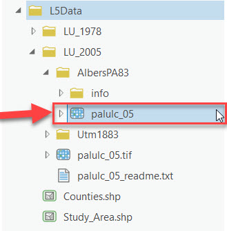
- Open a Catalog pane (Go to View tab, from the Window group > Catalog Pane) and explore the contents of the “LU_1978” and “LU_2005” folders. Notice that there are actually several different raster files in the 2005 folder. One is in a TIFF format (palulc_05) and the remaining two are in GRID format. We will use the dataset found in the "AlbersPA83" folder since it is already in the format and projection we need for this analysis.
- Add the "LU_1978" and "palulc_05" rasters to your map. If prompted with "Would you like to create pyramids?" select "No."
- Familiarize yourself with the contents of each data set to see similarities and differences between them. In particular, pay attention to the codes listed in the "VALUE" field of each attribute table. These are coded values representing land cover types, similar to the VEG_IDs from Lessons 3 and 4.
Raster attribute tables are different from vector attribute tables. Unlike with vector files, each unique value is only listed once.
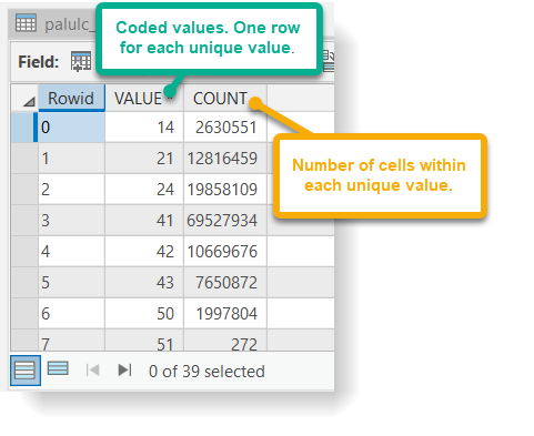
Do all of the land cover raster datasets have the same number of coded values? How many unique codes does each raster dataset contain? Are any of the codes the same? Do they have the same extent and cell size? Do all of the datasets have the same spatial reference information?
Part II: Customize the Land Cover Data and Perform the Analysis
Part II: Customize the Land Cover Data and Perform the Analysis
We want to figure out how land use has changed between 1978 and 2005 for several counties in southeastern Pennsylvania. We are mainly interested in the urbanization of agricultural and forested areas. You may have noticed that the land cover categories and coded values are different for the 1978 and 2005 datasets. Since we are interested in comparing land use change, we will need to standardize these categories before we can compare them. We also want to remove extraneous information from our datasets to make them easier to work with. We will use the Reclassification Tool in Spatial Analyst to perform both of these tasks simultaneously.
We will reclassify both of the input raster data layers using the standardized codes below. Codes 1, 2, and 3 collapse the existing detailed categories into broader categories. The "NODATA" (ALL CAPS) category allows us to ignore all of the land cover categories that we are not using in our analysis.
| Value | Category |
|---|---|
| 1 | Developed Land |
| 2 | Agricultural Land |
| 3 | Forested Land |
| NODATA | All Other Values |
The tables below show the original land cover codes from the 1978 and 2005 land cover grids, associated descriptions, and the new codes we will use to reclassify the data.
| Original value | Original Category | NEW Reclass Value |
|---|---|---|
| 11 | Residential | 1 |
| 12 | Commercial and Services | 1 |
| 13 | Industrial | 1 |
| 14 | Transportation, Communications... | 1 |
| 15 | Industrial and Commercial Complexes | 1 |
| 16 | Mixed Urban or Built-up Land | 1 |
| 17 | Other Urban or Built-up Land | 1 |
| 21 | Cropland and Pasture | 2 |
| 22 | Orchards, Groves, Vineyards | 2 |
| 23 | Confined Feeding Operations | 2 |
| 24 | Other Agricultural Land | 2 |
| 31 | Herbaceous Rangeland | NODATA |
| 32 | Shrub and Brush Rangeland | NODATA |
| 33 | Mixed Rangeland | NODATA |
| 41 | Deciduous Forest Land | 3 |
| 42 | Evergreen Forest Land | 3 |
| 43 | Mixed Forest Land | 3 |
| 51 | Streams and Canals | NODATA |
| 52 | Lakes | NODATA |
| 53 | Reservoirs | NODATA |
| 54 | Bays and Estuaries | NODATA |
| 61 | Forested Wetland | 3 |
| 62 | Non-forested Wetland | NODATA |
| 72 | Beaches | NODATA |
| 73 | Sandy Areas other than Beaches | NODATA |
| 74 | Bare Exposed Rock | NODATA |
| 75 | Strip Mines, Quarries, and Gravel Pits | NODATA |
| 76 | Transitional Areas | NODATA |
| Original value | Original Category | NEW Reclass Value |
|---|---|---|
| 14 | Roads | 1 |
| 21 | Row Crops | 2 |
| 24 | Pasture/Grass | 2 |
| 41 | Deciduous Forest | 3 |
| 42 | Evergreen Forest | 3 |
| 43 | Mixed Deciduous and Evergreen | 3 |
| 50 | Water | NODATA |
| 51 | Streams and Canals | NODATA |
| 52 | Lakes | NODATA |
| 61 | Forested Wetlands | 3 |
| 62 | Emergent Wetlands | NODATA |
| 70 | Bare; Unclassified Urban/Mines, Exposed Rock, Other Unvegetated Surfaces | NODATA |
| 111 | Residential Land; 5-30% impervious | 1 |
| 112 | Residential Land; 31-74% impervious | 1 |
| 113 | Residential Land; 74% < impervious | 1 |
| 121 | Institutional/Industrial/Commercial Land; 5 - 30% impervious | 1 |
| 122 | Institutional/Industrial/Commercial Land; 31 - 74% impervious | 1 |
| 123 | Institutional/Industrial/Commercial Land; 74% < impervious | 1 |
| 124 | Airports | 1 |
| 241 | Golf Courses | 1 |
| 750 | Active Mines/Significantly Disturbed Mined Areas | NODATA |
| 1111 | Residential Land; 5 - 30% impervious; Deciduous Tree Cover | 1 |
| 1112 | Residential Land; 5 - 30% impervious; Evergreen Tree Cover | 1 |
| 1113 | Residential Land; 5 - 30% impervious; Mixed Tree Cover | 1 |
| 1121 | Residential Land; 31 - 74% impervious; Deciduous Tree Cover | 1 |
| 1122 | Residential Land; 31 - 74% impervious; Evergreen Tree Cover | 1 |
| 1123 | Residential Land; 31 - 74% impervious; Mixed Tree Cover | 1 |
| 1131 | Residential Land; 74% <impervious; Deciduous Tree Cover | 1 |
| 1132 | Residential Land; 74% <impervious; Evergreen Tree Cover | 1 |
| 1133 | Residential Land; 74% < impervious; Mixed Tree Cover | 1 |
| 1211 | Institutional/Industrial/Commercial Land; 5 - 30% impervious; Deciduous cover | 1 |
| 1212 | Institutional/Industrial/Commercial Land; 5 - 30% impervious; Evergreen tree cover | 1 |
| 1213 | Institutional/Industrial/Commercial Land; 5 - 30% impervious; Mixed tree cover | 1 |
| 1221 | Institutional/Industrial/Commercial Land; 31 - 74% impervious; Deciduous Tree Cover | 1 |
| 1222 | Institutional/Industrial/Commercial Land; 31 - 74% impervious; Evergreen Tree Cover | 1 |
| 1223 | Institutional/Industrial/Commercial Land; 31 - 74% impervious; Mixed Tree Cover | 1 |
| 1231 | Institutional/Industrial/Commercial Land; 74% < impervious; Deciduous tree cover | 1 |
| 1232 | Institutional/Industrial/Commercial Land; 74% < impervious; Evergreen tree cover | 1 |
| 1233 | Institutional/Industrial/Commercial Land; 74% < impervious; Mixed tree cover | 1 |
After all of the time periods share common land cover codes, we can calculate how much change has occurred in each category over time using the workflow below:
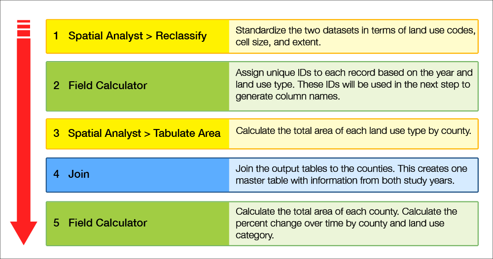
- Spatial Analyst > Reclassify: Standardize the two datasets in terms of land use codes, cell size and extent
- Field Calculator: Assign unique IDs to each record based on the year and land use type. These IDs will be used in the next step to generate column names.
- Spatial Analyst > Tabulate Area: Calculate the total area of each land use type by county
- Join: Join the output tables to the counties. This creates one master table with information from both study years.
- Field Calculator: Calculate the total area of each county. Calculate the percentage change over time by county and land use category.
-
Specify Geoprocessing Environment Settings
It is important to remember to double-check the environment settings within the Spatial Analyst tool pane, as ArcGIS sometimes ignores the global environment settings. A general rule of thumb is to always be certain of the environment settings used in your analysis, as they are critical to your results.
- Go to the Analysis tab, Geoprocessing group, Environments, verify that your workspace (Lesson 5 folder) and output coordinates (same as Study_Area) have been correctly set.
- We can remove portions of rasters by using the extent and mask settings. We’ll take advantage of this functionality to clip the two rasters to our study area.
- Under "Processing Extent", choose "Same as Layer Study_Area" as the extent.
- Under "Raster Analysis", choose the "Study_Area" as the mask.
- You typically want to use the same cell size as your coarsest dataset. Check the cell size of the 1978 and 2005 rasters (Properties > Source > Cell Size). Which one is the largest? Notice that both of the datasets have odd cell sizes with many decimal places. This is likely related to projection changes at some point during the preprocessing of the original data. We are going to pick "Maximum of Inputs".
- Finally, we want to ensure that we do not build pyramids for any layers. Pyramids will generalize data as you zoom out, which will reduce the visible accuracy of the displayed data. Scroll down to "Raster Storage", and uncheck Build.
- Click OK to save these settings. Save your project.
-
Reclassify the 1978 Land Use Data
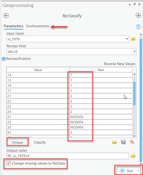
- Within the Analysis tab, Geoprocessing group go to Tools > Toolboxes > Spatial Analyst Tools > Reclass > Reclassify.
- Verify the Reclassify tool Environments settings (i.e., Output Coordinates - "Study_Area", Processing Extent - "Same as Layer Study_Area", Raster Analysis - Cell Size "Maximum of Inputs", Mask "Study_Area")
- Within the Parameters, Select "lu_1978" as the "Input raster" and "VALUE" as the "Reclass field."
- Click "Unique" to populate the "Values" column with the unique values in the dataset.
- Using the reclassification values given in Table 2, enter the appropriate values into the "New" column. Pay strict attention to the values you are entering to ensure proper reclassification.
- Name the new grid "RC_lu_1978.tif" and save it in your L5 folder.
Note: In ArcGIS, the default Output Raster format is a TIFF (.tif). - Check the "Change missing values to NoData" box.
- Click Run to perform the reclassification. Be patient as this may take a couple of moments depending on your computer’s configuration.
- If you’d like to review the progress, environment settings, and inputs, go to the Analysis tab, Geoprocessing group >History.
- "RC_lu_1978.tif" will be added to your map. Set the symbology so 1= red, 2= orange, and 3=green, and NoData = grey (Mask tab).
- Compare the output to the original raster. Right-click on the “lu_1978” layer in the Contents pane > Zoom to layer.
Notice how the extent setting we used clipped the raster to a much smaller area, and the mask setting we used assigned values of NoData to all of the areas that are both outside our study area boundary and within the extent.
Also, notice the grey areas within our study area. These are places that we reclassified the original land cover to "NoData." Keep in mind that you could also do the opposite of what we did – you can reclassify cells with starting values of "NoData" to other values.

Make sure you have the correct answer before moving on to the next step.
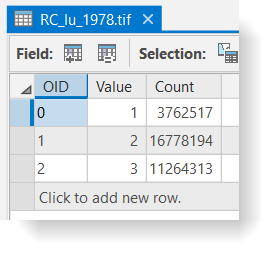
The cell counts in your RC_lu_1978.tif should match the examples below. If your data does not match this, go back and redo the previous step. You can double-check settings and rerun the tool in the Results window.
You’ll need right-click the RC_lu_1978.tif in Contents pane > Attribute table to see the Count attribute.
- Change the color of NoData back to “no color.”
- Since we no longer need the original land use layer, remove the lu_1978 grid from your map and Save the project.
-
Reclassify the 2005 Land Use Data
- Use the process from Step 2 and the values in Table 3 to reclassify "palulc_05” into a simplified land cover grid.
- Name the new grid "RC_LU_2005.tif"
- Add "LU_2005_RC" to your map and set the symbology so 1= red, 2= orange, and 3=green, and NoData = grey.
- Compare the output to the original raster. Right-click on the “lu_2005” layer in the Contents pane > Zoom to layer.
How did the extent, mask, and cell size settings affect the output raster? You can view the cell size settings by right-clicking on the output raster > Properties > Source > Cell Size.
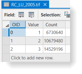
Make sure you have the correct answer before moving on to the next step.
Your LU_2005_RC grid should match the example below. If your data does not match this, go back and redo the previous step.
- Change the color of NoData back to “no color.”
- Since we no longer need the original land cover layer, remove the "palulc_05" grid from your map and Save the project.
Since you know the cell size and number of cells with each unique value, you can easily calculate the total area within each land cover category for the entire study area. Note that you need to use the area of the cell, not the length, when making these calculations.
-
Add Unique Identifier
In the next step, we will use the "Tabulate Area" tool to create a table with the areas of each land cover type within each county. We will repeat this for both time periods. The "Tabulate Area" tool will automatically generate column names based on the values in the input table. Since we will have two datasets with the same land cover codes, we need to be able to keep track of each year’s corresponding table. To do this, we will add new fields to each reclassified raster attribute table and populate them with a combination of the study year and the land cover code.
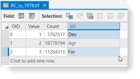
- Right now, the land covers are represented by arbitrary codes of 1, 2, and 3. We are going to assign more meaningful names (three letter abbreviations) so we don’t confuse the numeric codes later on. Open the RC_lu_1978.tif attribute table and add a new text field called “lu” with a length of 3.
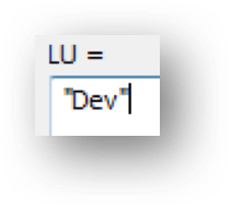
- Select the first row (VALUE = 1) and use the calculate field to assign a value of “Dev.”
- Repeat for the remaining rows as shown below and then Save your edits.
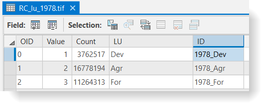
- Add a new text field named "ID" with a length of 8 (4 characters for the year, one character for a "_", and three characters for the land use abbreviations).
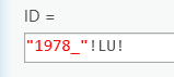
- Set the values of the ID field to be equal to "1978_"!LU!. This will create a unique ID for each land use code and year. For example, the first row has a value of Dev, so the ID field would be set to "1978_Dev".
- View the results to make sure your calculation worked as planned. Close the attribute table.
- Repeat for the 2005 data. Make sure you use the correct year in your calculations.
- Clear the selected features and save your map. (If you skip this step, future operations will only be run on the fields you have selected).
Make sure you have the correct answer before moving on to the next step.
Your reclassified attribute tables should have their ID values populated as shown below. If your data does not match this, go back and redo the previous step.
 Click for a text alternative to the image above.
Accessible Version of Data Above, 1978 OID Value Count LU ID 0 1 3762517 DEV 1978_Dev 1 2 16778194 Agr 1978_Agr 2 3 11264313 For 1978_For 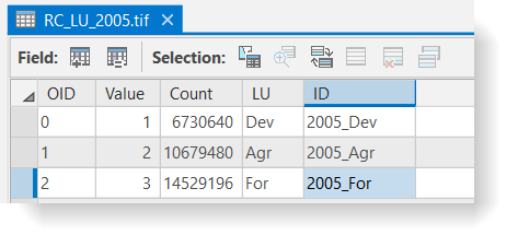 Click for a text alternative to the image above.
Accessible Version of Data Above, 2005 OID Value Count LU ID 0 1 6730640 Dev 2005_Dev 1 2 10679480 Agr 2005_Agr 2 3 14529196 For 2005_For
-
Tabulating Areas of the Land Use Grids
Now that we have reclassified the land cover data with standardized categories and created unique IDs, we can begin our land use change analysis. We need to calculate the area for each of the three land cover categories within each county for each time period. To do this, we will use the "Tabulate Area" tool. This tool calculates cross-tabulated areas between two datasets. This tool summarizes one dataset within regions specified by a second data set.
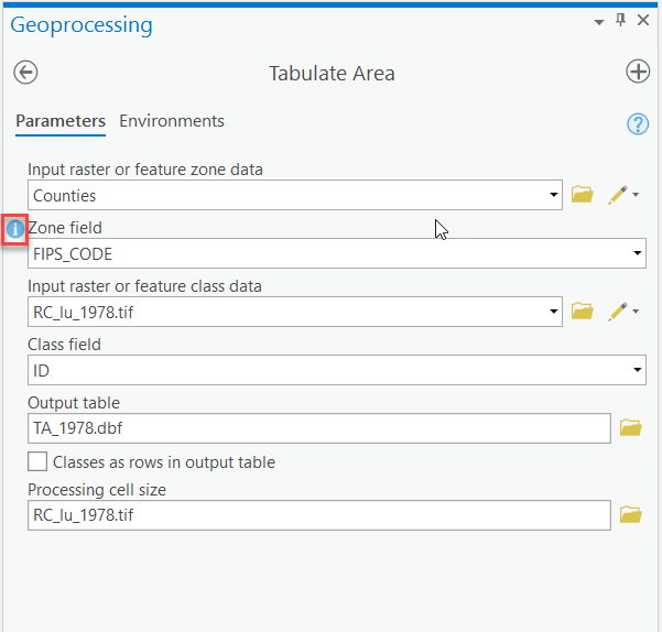
- Within the Analysis tab, Geoprocessing group go to Tools > Toolboxes > Spatial Analyst Tools > Zonal > Tabulate Area.
- Select "Counties" as the "Input raster or feature zone data" layer and "FIPS_CODE" as the "Zone field." The FIPS_CODE is a national naming convention system (similar to zip codes), that assigns a unique code to each county.
- Select RC_lu_1978.tif as the "Input raster or feature class data" layer and "ID" as the "Class field."
- Name the Output table "TA_1978.dbf" and save it in the L5 folder. Be sure to include the .dbf extension at the end of your file name to create a dBase table. Failure to add this file extension will result in an INFO table, which has different functionality than a DBF file. You will encounter trouble later in the lesson if you skip this small step.
- Make sure to read the embedded help topics about what each parameter controls.
- Leave the default processing cell size and click Run to tabulate the areas.
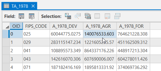
Open the "TA_1978.dbf" table in your map. Notice the names of the columns. What are the units of the tabulated areas?
- Repeat this process for the 2005 reclassified raster using "ID" for the class field. Name the output table "TA_2005.dbf.”
Make sure you have the correct answer before moving on to the next step.
Your tabulated area tables should match the examples below. Both of the tables should have 19 records and 5 columns. If your data does not match this, go back and redo the previous step.
 Click for a text alternative to the image above.
Sample Data 1978 OID FIPS_CODE A_1978_Dev A_1978_AGR A_1978_FOR 0 025 60044775.0275 140076533.603 764621228.308 1 029 283115147.234 1221605255.57 451162509.312 2 041 108895573.345 864337176.226 448917213.30 3 043 142616070.306 607690006.007 604278011.426 4 071 187182416.169 1895813331.92 374069736.292 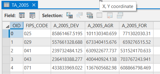 Click for a text alternative to the image above.
Sample Data 2005 OID FIPS_CODE A_2005_Dev A_2005_AGR A_2005_FOR 0 025 85861467.5195 101130340.659 771302030.31 1 029 557661328.688 673340415.676 659276515.52 2 041 239732484.125 630922677.737 531524170.633 3 043 236418388.277 400440924.138 703767243.941 4 071 433833969.022 1367605682.98
608866798.469
-
Create a Master Table of the Two Tabulate Area Tables
We will use the Join function to create a "master table” that contains the information from both of the Tabulate Area tables and the attributes of the counties. Since a joined table contains only virtually referenced information, we will export this dataset, thus permanently saving the joins.
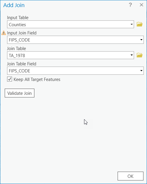
- Right-click on the "Counties" shapefile and choose Joins and Relates > Add Join. Use the settings below and click "Validate" and then "OK". There may be a warning about the .dbf file not being indexed, it is OK to proceed.
- Open the "Counties" attribute table to view the join. Notice how the FIPS_CODE’s match up with County Names.
- Right-click on the "Counties" shapefile again and create another join between the TA_2005 table based on the "FIPS_CODE." Open the "Counties" attribute table to view the second join. Your "Counties" attribute table should now have fourteen columns.
- You may notice that some of the field names are redundant. We will remove these by using a trick before exporting our data to make the joins permanent.
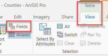
- Go to the Table > View tab and select Fields by unchecking the highlighted fields below and click Save.
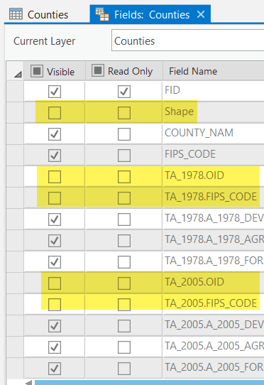
- Close the Counties attribute table if it is open and then open the attribute table again to see the results.
Make sure you have the correct answer before moving on to the next step.
Your attribute tables should match the examples below. If your data does not match this, go back and redo the previous step.
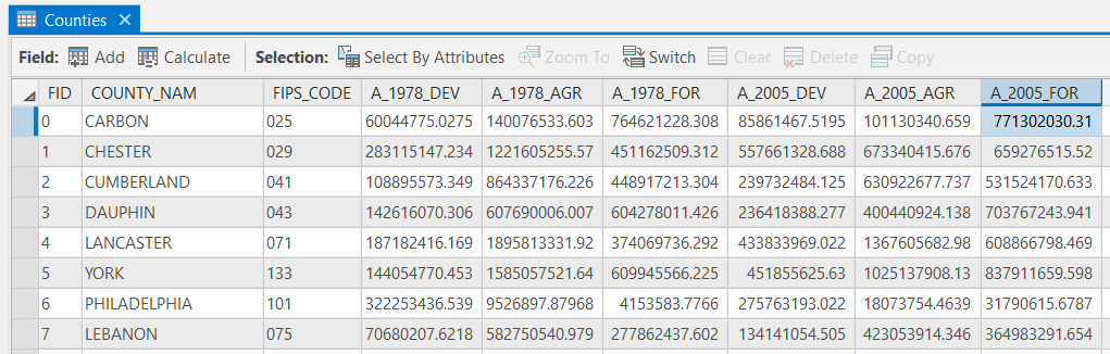 Click for a text alternative to the image above.
Sample Data, Counties FID county_Nam FIPS_code A_1978_Dev A_1978_agr A_1978_for A_2005_Dev A_2005_agr A_2005_for 0 Carbon 025 60044775.027 140076533.603 764621228.308
85861467.5195 101130340.659
771302030.31 1 Chester 029 283115147.23 1221605255.57 451162509.312 557661328.68 673340415.676
659276515.52 2 Cumberland 041 108895573.349 864337176.226
448917213.304 239732484.125 630927677.737 531524170.633 3 Dauphin 043 142616070.306 607690006.007 604278011.426 236418388.277 400440924.138 703767243.941 4 Lancaster 071 187182416.169 1895813331.92 374069736.292 433833969.022 1367605682.98 608866798.469
5 York 133 144054770.453 1585057521.64
609945566.225
451855625.63 1025137908.13
837911659.598 6 Philadelphia 101 322253436.539 9576897.87968 4153583.7766 275763193.022 18073754.4639 31790615.6787 7 Lebanon 075 70680207.6218 582750540.97 277862437.60 134141054.505 423053914.346 364983291.654 - Right-click on the "Counties" shapefile and choose Data > Export Features. Be sure to export all records and name it "LU_Change" in your L5 folder. Select "Yes" to add the shapefile to your map. Review the results.
- Right-click on the "Counties" shapefile and choose Joins and Relates > Remove Joins > Remove All Joins.
- Save your project.
- Right-click on the "Counties" shapefile and choose Joins and Relates > Add Join. Use the settings below and click "Validate" and then "OK". There may be a warning about the .dbf file not being indexed, it is OK to proceed.
-
Calculate the Area of Each County
- To identify the percent change over time for the three land-use layers, we first need to calculate the area of each county. Open the "LU_Change" attribute table and add a new float field called "TotAreaSQM" and Save. We need to use a float type since our numbers exceed the limits for short and long integers.
- Close the "LU_Change" attribute table.
- Reopen the "LU_Change" attribute table and populate the "TotAreaSqm" field using the "Calculate Geometry" tool. Make sure you use units of square meters.
Sometimes your calculated values will have too many digits to be stored in a long integer field. In these situations, you can use a data type of "float" instead.
-
Calculate the Percent Change Over Time By County and Time Period
As we saw in Lesson 2, it is much easier to compare numbers using percent areas vs. calculated areas. In this step, we are going to calculate the percent change within each land use type between 1978 and 2005.
- Before we can complete the calculations, we need to add new fields to hold the results. Add three new short integer fields using the names below.
- PctChg_dev
- PctChg_agr
- PctChg_for
- We are going to use a semi-complicated equation to avoid the extra steps of calculating the percent area of each category, in addition to calculating the percent change over time. The basic equation we will use is:
Note: Although you can represent a percentage as a fraction, multiplying that fraction by 100 will give you a range of 0 to 100%.
([ tot land use in later time] - [ tot land use in earlier time]) / [TotAreaSqm]) * 100
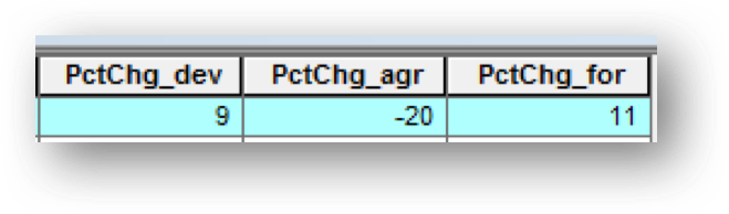
- Calculate the percent change for each of the three new fields using the equation above. For example, to calculate the field "PctChg_dev," the equation would be:
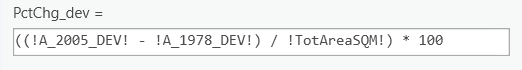
Make sure you have the correct answer before moving on to the next step.
Your calculated values should match the example below. If your data does not match this, go back and redo the previous step. I have only included the values for Adams County. You may need to sort your results to find this county.
- Before we can complete the calculations, we need to add new fields to hold the results. Add three new short integer fields using the names below.
-
Visualize Your Results Using Maps
Create a map layout with the 4 map frames below. (Note: You will not turn in these maps. However, you will need to consult them to complete the Lesson 5 Quiz).
- One data frame showing the agricultural land cover change between 1978 - 2005.
- One data frame showing developed land cover change between 1978 - 2005.
- One data frame showing forest land cover change between 1978 - 2005.
- One data frame with a locator map.
- Label each county with the % land cover change.
- Select a consistent color scheme that allows you to compare the three maps (e.g., red = increase, green = decrease, gray = no change)
In Lesson 5, we used the Reclassify Tool to collapse complex categories into simpler versions. We also used it to eliminate portions of our starting data that we did not need for our analysis using the "NoData" code. Can you think of any other ways you could use this tool?
That’s it for the required portion of the Lesson 5 Step-by-Step Activity. Please consult the Lesson Checklist for instructions on what to do next.
Try This!
Try one or more of the optional activities listed below.
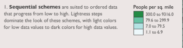
- Use the Color Brewer [26] website to help you choose symbology that highlights trends and spatial patterns in your data.
- Use the USDA/NRCS Geospatial Data Gateway Site to download land use data for an area of interest. Try reclassifying the data using the standardized categories from this lesson.
- Download the municipal boundaries for Pennsylvania using the PASDA site. On the home page, click on the “Boundaries” shortcut and select "Pennsylvania municipality boundaries." Use this file to define your zones instead of the county boundaries.
Advanced Activity
Advanced Activity
Advanced Activities are designed to make you apply the skills you learned in this lesson to solve an environmental problem and explore additional resources related to lesson topics.
Directions:
In the Step-by-Step portion of the lesson, we were mainly concerned with three land cover categories: developed, agriculture, and forest. We are also interested in how wetlands have changed between 1978 and 2005. We are particularly interested in the land cover categories below:
- 1978 Land Cover Categories: "Forested Wetland" and "Non-forested Wetland"
- 2005 Land Cover Categories: "Forested Wetlands" and "Emergent Wetlands"
We would like to figure out the following:
- How many counties contain wetlands in 1978 and 2005?
- Which locations have the most wetlands in 1978 and 2005?
Note: You may want to read the related quiz questions within the Lesson 5 Quiz before completing the activity so you know what information to look out for.
Summary and Deliverables
Summary and Deliverables
In Lesson 5, we determined land use change between 1978 and 2005 using land cover datasets from two different sources. We explored how standardizing data can be useful in comparing different, yet similar, datasets by utilizing reclassification tools. Then we calculated percent differences by determining the percent area for each land cover category and combining this information into one table using simple math.
Lesson 5 Deliverables
Lesson 5 is worth a total of 100 points.
- (100 points) Lesson 5 Quiz
Tell us about it!
If you have anything you'd like to comment on, or add to the lesson materials, feel free to post your thoughts in the Lesson 5 Discussion. For example, what did you have the most trouble with in this lesson? Was there anything useful here that you'd like to try in your own workplace?
Additional Resources
Additional Resources
This page includes links to resources such as additional readings, websites, and data related to the lesson concepts. Feel free to explore these on your own. If you would like to suggest other resources for this list, please send the instructor an email.
Additional Readings:
- A 125 Year History of Topographic Mapping and GIS in the U.S. Geological Survey 1884-2009, Part 2 [27]
- A Land Use And Land Cover Classification System For Use With Remote Sensor Data [28]
Websites:
- USDA/NRCS Geospatial Data Gateway [29]
- Greening the Lower Susquehanna [30]
- United States Geological Survey (USGS) Earth Resources Observation and Science Center [31]
- NASA Land Cover and Land Use Change Program [32]
- National Land Cover Database factsheet [33]
- Environmental Protection Agency (EPA) Multi-Resolution Land Characteristic Consortium (MRLC) [34]:
- National Oceanic and Atmospheric Administration (NOAA) Office or Coastal Management Digital Coast [35]
Additional Land Use Data:
- Global Land Survey [36](historic NASA and the USGS collaboration from 2009 through 2011)
- Global Land Cover Data [37] (Product Search, AVHRR Global Land Cover Product)
- NASA Goddard Space Flight Center MODIS Land Cover Data [38]