Lesson 6: Forests, Carbon Sequestration, and Climate Change
Lesson 6 Overview and Checklist
Lesson 6 Overview and Checklist
Scenario
You have been hired by a local landowner to calculate the carbon sequestration potential of a small forested area in southeastern Michigan. You know it is possible to estimate carbon values using measurements of tree height and diameter. After an initial site visit to the property, you determine it will be too costly and time-consuming to measure every single tree on the property. Given these limitations, you decide to use a representative sample to estimate values for the entire forest. After setting up a sampling plan, you collect information in the field for 18 sample areas. After returning to the office, you enter your data into two CSV files, one with tree measurements and plot identification numbers and another with plot GPS coordinates. You get to use ArcGIS and the Spatial Analyst extension to create a plot shapefile from your tabular data and interpolate your sample data for the entire forest.
Goals
At the successful completion of Lesson 6, you will have:
- created shapefiles from tabular coordinate data;
- interpolated point data to raster grids;
- customized the Spatial Analyst environment settings.
 |
 |
 |
 |
 |
Questions?
If you have questions now or at any point during this lesson, please feel free to post them to the Lesson 6 Discussion.
Checklist
This lesson is worth 100 points and is one week in length. Please refer to the Course Calendar for specific time frames and due dates. To finish this lesson, you must complete the activities listed below. You may find it useful to print this page out first so that you can follow along with the directions. Simply click the arrow to navigate through the lesson and complete the activities in the order that they are displayed.
- Read all of the pages in Lesson 6.
Review the information on the "Background Information," "Required Readings," "Lesson Data," "Step-by-Step Activity," "Advanced Activities," and "Summary and Deliverables" pages. - Read or review required readings.
See the "Required Readings" page for links to help topics. - Download Lesson 6 datasets.
See the "Lesson Data" page. - Download and complete the Lesson 6 Step-by-Step Activity.
See the "Step-by-Step Activity" page for a link to a printable PDF of steps to follow. - Complete the Lesson 6 Advanced Activity.
See the "Advanced Activity" page. - Complete the Lesson 6 Quiz.
See the "Summary and Deliverables" page. - Optional - Check out additional resources.
See the "Additional Resources" page. This section includes links to several types of resources if you are interested in learning more about the GIS techniques or environmental topics covered in this lesson.
SDG image retrieved from the United Nations [1]
Background Information
Background Information
The Role of Forests in Climate Change
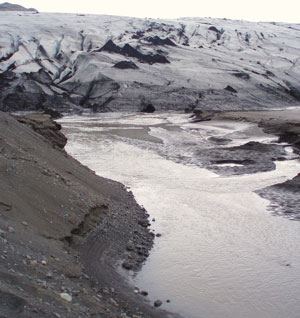
Calculating carbon sequestration and associated carbon credits for forests is an initiative related to climate change. Climate change, also known as global warming, is caused by increased levels of greenhouse gases trapped in Earth’s atmosphere. Some of the expected effects of global warming include melting glaciers, sea-level rise, changes in water resources, changes in food production, loss of biodiversity, increases in extreme weather, and threats to human health.
Forests play an important role in climate change due to the fact that trees naturally absorb and release carbon dioxide during their life cycle. During photosynthesis, they remove carbon dioxide from the air and store it as organic matter in their trunks, branches, foliage, roots, and soils. This process is known as carbon sequestration. When trees decay or burn, they release their stored carbon back into the atmosphere. The amount of carbon a particular tree absorbs or releases throughout its lifecycle is negligible. However, due to their global abundance, the cumulative effect is very large.
The Intergovernmental Panel on Climate Change (IPCC) [2], winner of the 2007 Nobel Peace Prize, is the United Nations body for assessing the science related to climate change and, therefore, often considered the world’s leading authority on climate change. One of their recommendations is that we need to mitigate the future impacts of climate change by reducing current and future emissions. One way to reduce emissions is to reduce the number of forests that are clear-cut or degraded since these activities account for about 15% of global greenhouse gas emissions. There are simply some existing natural environments that we cannot afford to lose due to their irrecoverable carbon reserves. And, preserving existing forests is considered a much better alternative to reforestation or afforestation, as it takes decades for a new tree to grow and absorb the amount of carbon that is released when a mature tree is lost.
There are several initiatives to encourage the preservation of existing forests on a global scale. Reduced Emissions from Deforestation and Forest Degradation (REDD+) [3] is a framework by the UNFCCC (United Nations Framework Convention on Climate Change) Conference [4] that guides activities that will provide financial compensation to landowners for maintaining and protecting forests. To receive compensation under the REDD+ initiative, landowners need to be able to assess the amount of carbon that is stored in the trees on their property. Many of the methods to do this require a forest inventory in which tree species, height, and diameter at breast height (DBH) are measured. This information is used to estimate the volume of organic matter for each tree, which is then translated into results-based financing, whose value fluctuates depending on the current market trading value of carbon.
Field Data Collection & Representative Samples
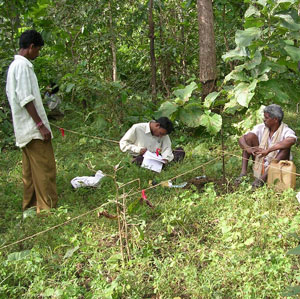
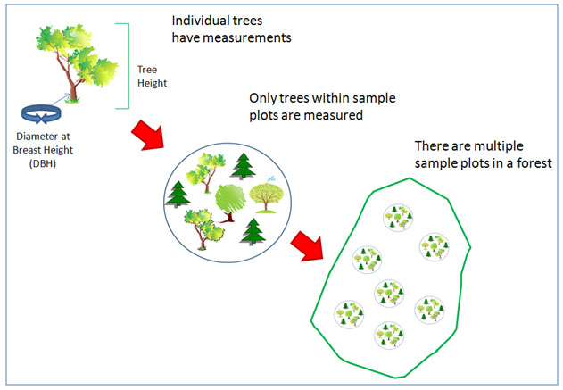
While it would be more accurate to measure every tree in a forest during field inventories, limitations of time and money typically make this unfeasible. This is especially true for large or hard-to-access areas (e.g., mangrove forests, swamp forests, forests with steep topography). Therefore, a common practice has been to collect a representative sample and then interpolate the values for the entire study area or use remotely sensed data. In this activity, we will concentrate our efforts on a representative sample. Forests can be inventoried by demarcating a number of sampling locations known as plots. Trees are only measured if they fall within the plot boundaries. The number and location of plots required for a given area depend on the size of the forest and the amount of variation within the study area. Large forests or forests with a lot of variation in tree cover will require more plots than small forests or forests with uniform tree cover.
GIS can be very helpful when trying to decide on the number and location of sample plots. For example, you can overlay your site boundary with current and historical aerial photos to look for variations in forest cover. You can also incorporate other datasets such as Digital Elevation Models (DEMs), hydrology, parcel boundaries, and roads. These datasets will help you identify possible hazards in the field such as fences, large rivers, steep terrain, etc. They can also help you estimate the age of the forest, depending on how old the forest is and how far back you can find aerial photos.
Most of these concepts are not unique to forest inventories. It is actually quite common in the environmental field to use representative samples to understand larger areas. For example, environmental consultants typically install monitoring wells to understand how groundwater and soil conditions vary across a site. By measuring water levels in the monitoring wells, they are able to calculate the direction and speed of groundwater flow for the whole site. They also collect groundwater and soil samples at these locations to determine if pollution levels exceed legal limits. Since the locations of the samples are known, it is possible to plot them on a map and use their location to predict values between monitoring wells.
Interpolating Sample Data with Spatial Analyst
After data is collected in the field, it is common to enter the data into an electronic format such as an Excel table, CSV file, or a simple database. As long as the field measurements are in a digital format, it is possible to view them in ArcGIS. Depending on the native file type, you may need to complete some intermediate processing steps for ArcGIS Pro to recognize them. Using the "Join" and "Display XY Data" tools in ArcGIS, it is possible to create shapefiles from tabular data. You can then use your shapefiles to identify spatial patterns in your data and create maps of your results.
The interpolation tools available within the ArcGIS Spatial Analyst Extension are particularly helpful when working with representative point data. In Lesson 6, we will practice interpolating point data to estimate values for areas that were not actually sampled. We will also explore how the options and environment settings listed below affect the output grids created by Spatial Analyst tools. We will read more about these settings in the help articles listed in the required readings section.
- Cell Size: Specifies how coarse or fine the resolution of the output raster will be. Cell size is specified by the length of each cell in the output raster. Since pixels are square, the length and width will always be the same value. You can use the cell size to calculate areas of raster grids using the equation "length * width * the number of cells." A common mistake is to assume the units of cell size refer to the area instead of length. The units of cell size are the same as the units of the coordinate system stored with the data. The calculated area of a raster will vary depending on the cell size you specify.
- Extent: The overall size and location of your output rasters, defined as the coordinates of the lower-left cell and the coordinates of the upper-right cell. This setting is often confused with the mask setting.
- Mask: Specifies the portions of the output raster that will be assigned calculated values as opposed to "NoData." This setting is often confused with the extent setting. You can also use a combination of extent and mask settings to mimic the clip and union tools used for vector files.
- Output Coordinate System: The reference coordinate system for the output files. Modifying this setting is one way to project raster files.
- Work Space: The folder (pathname) where your output files will be saved. Spatial Analyst performs better if your input and output files are saved in the same directory.
Required Readings
Required Readings
The required readings for Lesson 6 are listed below. Each of the short articles provides specific information about the tools and techniques we will use in Lesson 6.
Esri Help Topics
Find the help articles listed below on ArcGIS Pro Resources Center [5] website.
- "What is the ArcGIS Spatial Analyst Extension? [6]"
- "An Overview of the Spatial Analyst Toolbox [7]"
- "The Analysis Environment of Spatial Analyst [8]"
- "Geoprocessing Environment Settings [9]"
- "An Overview of the Interpolation Toolset [10]"
- "How IDW Works [11]"
- "An Overview of the Zonal Toolset [12]"
Lesson Data
Lesson Data
This section provides links to download the Lesson 6 data along with reference information about each dataset (metadata). Briefly review the information below so you have a general idea of the data we will use in this lesson.
Lesson 6 Data Download:
Note: You should not complete this activity until you have read through all of the pages in Lesson 6. See the Lesson 6 Checklist for further information.
Create a new folder in your GEOG487 folder called "L6." Download a zip file of the Less
Metadata
Publicly Available Data:
Base Map:
- Source: ESRI Resource Center (see Lesson 2 for more details about this site)
- Service Names: OpenStreetMap
- Within ArcGIS Pro, go to the Map tab, Layer group > Basemap.
Private Data (Located Inside the Lesson 6 Folder):
The data we will use In Lesson 6 was collected by the International Forestry Resources and Institutions (IFRI) Organization [14]. IFRI is a research network made up of 18 collaborating research centers around the globe. Since 1992, IFRI researchers have collected both ecological and social field data for over 400 sites in 15 countries. For this lesson, we are going to use a subset of their data to calculate the carbon sequestration and carbon credits for a small forest located in southeastern Michigan.
The data was collected by laying out 18 circular plots, every 10 meters in diameter, at random locations throughout the study forest. The coordinates of these locations were determined in advance using GIS. In the field, students used GPS and mobile apps to navigate to the middle of each plot, lay out the circular plot, and collect attribute information about the trees. Any trees that fell inside the plot boundaries were measured to obtain their height and diameter. Measurements were collected for a total of 278 trees.
- Parcel_Boundary: (Polygon shapefile) The boundary of the property where the study forest is located.
- Forest_Boundary: (Polygon shapefile) The boundary of the study forest.
- Plots: (CSV file) Table containing the GPS coordinates of plots along with their ID numbers.
- Tree Measurements: (CSV file) Table containing the field measurements of trees (diameter and height), along with the plot ID number where each tree is located.
- Vegetation07: (Polygon shapefile) Polygons representing homogeneous units of forest cover/age.
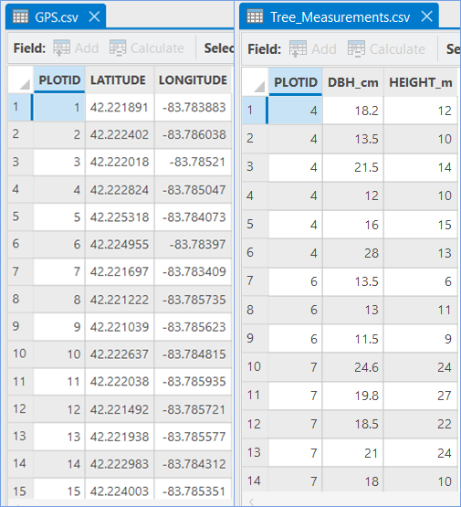 Figure 4: The GPS and Tree_Measurement tables both contain field measurements. Since they share an ID field (PLOTID), they can be joined together in GIS.
Step-by-Step Activity
Step-by-Step Activity: Overview
Step-by-Step Activity: Overview
The Step-by-Step Activity for Lesson 6 is divided into two parts. In Part I, we will create a point shapefile from our starting data tables. We will then use the field calculator to calculate the carbon sequestration for each tree and create totals by plot. In Part II, we will use the Spatial Analyst extension tools to interpolate the plot data to a raster grid covering the entire study area. We will use the results to calculate the total carbon for the study forest. During interpolation, we will experiment with several different toolbar settings to see how they affect the results.
Lesson 6 Step-by-Step Activity Download
Note: You should not complete this step until you have read through all of the pages in Lesson 6. See the Lesson 6 Checklist for further information.
Part I: Create Shapefile from Field Data Tables
Part I: Create Shapefile from Field Data Tables
In Part I, we will create the shapefile we will use to interpolate our data (a point shapefile of plots with the total carbon as an attribute). To create this, we start with the two CSV files "GPS.csv" and "Tree _Measurements.csv".
-
Familiarize Yourself with the Study Area
- Create a New Map and save your project to the L6 folder without creating a new folder for the project.
- Add the parcel boundary and forest boundary from your L6Data folder to your Map.
- Change the parcel and forest boundaries symbols to hollow outlines.
- Go back to the Map tab and add the "OpenStreetMap" and “Imagery Hybrid” Basemaps to your Map.
- Use the Explore tool to pan and zoom within the surrounding area. Notice how the imagery shows that only the southern portion of the parcel is forested.

How far is the study forest from the city of Ann Arbor, MI or State College, PA? What is the surrounding land used for (commercial, agriculture, residential, etc.)?
- Confirm the coordinate system of the Map is set to “NAD 1983 UTM Zone 16N.” If yours does not match, right-click on the Lesson 6 Map in the Contents pane > Properties > Coordinate System > Projected Coordinate Systems Folder > UTM > NAD 83 > NAD 1983 UTM Zone 16N. Save your project to lock in the settings.
-
Create Plot Shapefile from GPS Data Table
- Add the "GPS.csv" file from your L6Data folder to your map and explore the attributes.
- Open the table and explore the attributes. What spatial reference do you think the x and y coordinates refer to?
- Right-click on the GPS table in the Contents pane > XY Table To Point
- X Field: LONGITUDE
- Y Field: LATITUDE
- Z Field: <None> (since we are not interested in height)
- Coordinate System: GCS_WGS_1984

- Right-click on the "GPS_XYTabletoPoint" layer in the Contents pane > Data > Export Features and export to a new shapefile in your L6 folder. Name it "Plots." Make sure you establish the output coordinate system under Environments as NAD_1983_UTM_Zone_16N.
- The "Plots" shapefile will be added to the Map, remove the GPS_XYTabletoPoint layer, and the GPS table from your Contents pane and Save the project.
Make sure you have the correct answer before moving on to the next step.
Check the Properties > Source Tab > Spatial Reference to make sure the Plot shapefile was projected correctly to NAD 183 UTM Zone 16N. If your projection doesn’t match, make sure you remove the base maps, and choose the coordinate system of the Map.

Make sure you have the correct answer before moving on to the next step.
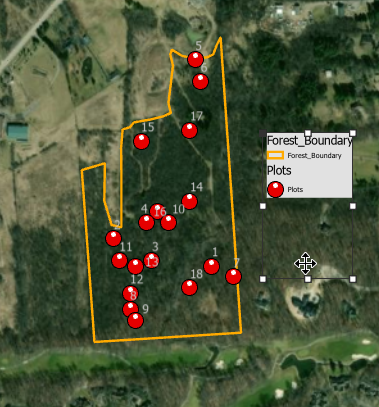
Check the location of your plots by comparing your plot shapefile to the map below. Note: Your map will not look exactly like this by default. I changed the symbology of the points, added labels of Plot ID's, and added the Imagery layer in the background to make it easier to compare your data to the example. If you add the imagery base map again, make sure you remove it from your map and Save before moving on to the next step.
-
Calculate the Carbon Sequestered by Each Tree
- Add the tree measurements CSV file from your L6Data folder to your map and explore the attributes. What does DBH mean?
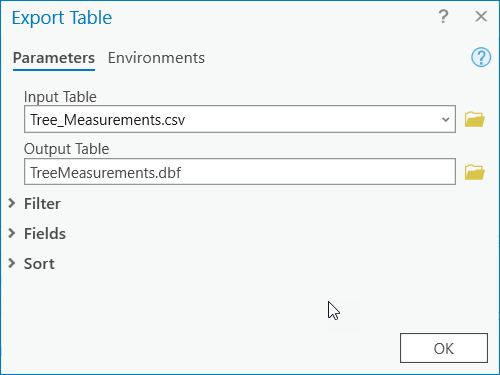
- We need to add several new fields to the table to calculate the carbon values for each tree. ArcGIS will not allow you to add new fields to a CSV file. Export it to a .dbf file of the same name using the export option listed in the dropdown menu in the upper left corner of the attribute table. Make sure to select the file type as dBASE table so it has the “.dbf” extension. Add the resultant file to your map.
 [15]
[15] - Remove the "Tree_Measurements" CSV file from your Map and Save the project.

We are going to use a somewhat general set of equations to estimate the carbon stored in each tree. For this lesson, we do not need a high level of accuracy. The important part is to demonstrate the concept of how one can calculate carbon credits using GIS. You can read more about the method we will use at: How to calculate the amount of CO2 sequestered in a tree per year [16].
There are more sophisticated methods you can use that take into account the tree species, age, climate, and other factors. The paper, “Methods for Calculating Forest Ecosystem and Harvested Carbon with Standard Estimates for Forest Types of the United States [17]” highlights an example of a more complex methodology. An example of a simpler method is highlighted in the “Landowner’s Guide to Determining Weight and Value of Standing Pine Trees [18]”.
- Add 7 new double fields to the Tree_Measurements dbf table. Save
 the changes after you have added the fields. Use the names below:
- DBH_in (this is to convert units from cm to in)
- Height_ft (this is to convert units from m to ft)
- Wa_lbs (above ground tree weight)
- Wt_lbs (total tree weight with roots)
- Wd_lbs (dry tree weight)
- Wc_lbs (weight of carbon)
- Ws_lbs (weight of carbon dioxide sequestered)
- Use the calculate field tool and the equations below to populate the new fields from step d.
Variable Description Units Equation D Measured tree diameter (DBH) Inches See Tree Measurements Table (be careful with your units here). H Measured tree height Feet See Tree Measurements Table (be careful with your units here). Wa Total above-ground weight of the tree (w/o roots) Pounds Wa = 0.15D2 *H Wt Total weight of the tree and roots Pounds Wt = 1.2 Wa Wd Dry weight of the tree Pounds Wd = 0.725Wt Wc Weight of carbon in the tree Pounds Wc = 0.5Wd Ws Weight of carbon dioxide sequestered in the tree Pounds Ws=3.6663Wc Tips for Success:
- Don’t forget to convert units when necessary. Check Online Conversion.com [19] if you are unsure of the conversion equations. Round the conversion factors to the nearest 4 decimal places (e.g., 0.3937007874 = 0.3937). What is the conversion factor for meters to feet?
- Make sure to use double as the data type.
- Remember that you have the option to undo.
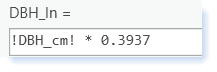
- To calculate D2 in the Python 3, multiply D * D or D**2 (e.g., 0.15 * !DBH_In!**2 * !Height_ft!)
- The example below shows the equation you would type into the calculate field (Python 3) to convert the DBH values from centimeters to inches.
Make sure you have the correct answer before moving on to the next step.
Compare your data with the summary statistics below for the "Ws" variable.
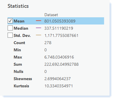 Click here for an accessible version of the data above
Statistics Shown in the image above Mean 801.0505393089 Median 337.511190219 Std. Dev. 1,171.7755087661 Count 278 Min 0 Max 6,748.03406916 Sum 222,692.04992788 Nulls 0 Skewness 2.6994064237 Kurtosis 10.3340354971 If your data does not match this, go back and redo your calculations. Pay special attention to unit conversations (make sure to round to the nearest 4 decimal places), data types of the fields you used, and typos in equations.
-
Combine the Carbon Calculations with the Plot Shapefile
Ultimately, we want to join the calculations from Step 3 to the plot shapefile we created in Step 2. However, we can’t do this directly, because there is more than one entry in the tree measurement table for each plot in the shapefile. We know this is true because there are 278 trees but only 18 plots. Before we can join the two files, we need to summarize the tree data to the plot level.- Calculate the total carbon sequestered per plot. Open the "Tree_Measurement" dbf table. Right-click on the "PLOTID" field>Summarize. Use the settings shown in the following figure. Make sure the extension is a .dbf file.
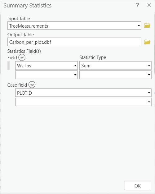
- The "Carbon_per_plot" table will be added to your map. Notice there are only 18 records now instead of 278. The "FREQUENCY" is the number of trees within each plot. (Now is a good time to change the field alias to “Number _Trees” so you remember what this means later on. Right-click on the field > Field > alias.) The "Sum_Ws_lbs" is the total carbon sequestered for all trees within the plot.
- Now we know the total carbon sequestered for each plot. However, we still need to normalize this data before we can interpolate it since we’re estimating carbon values across the entire area where there aren’t any additional plots. Because the diameter of each plot is 10 meters, we know the area of each plot is 78.5 square meters. By dividing each carbon total by this area, we derive a “carbon per square meter” value, which can be interpolated across the entire study area.
- Add a new double field named "c_lbsqm" to the "Carbon_per_plot" table. Calculate the pounds of carbon sequestered per square meter for each plot.
Make sure you have the correct answer before moving on to the next step.
Compare your data with the summary statistics below for the "c_lbsqm" variable.
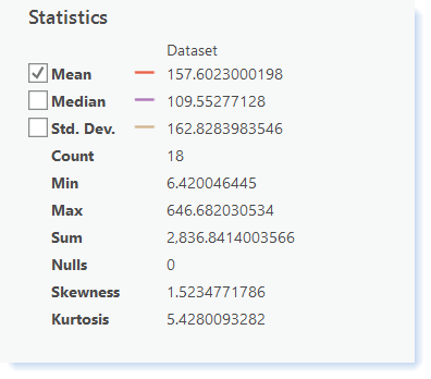 Click here for an accessible version of the data above
Statistics Shown in the image above Mean 157.6023000198 Median 109.55277128 Std. Dev. 162.8283983546 Count 18 Min 6.420046445 Max 646.682030534 Sum 2,836.8414003566 Nulls 0 Skewness 1.5234771786 Kurtosis 5.4280093282 If your data does not match this, go back and redo your calculations.
- Join the "Carbon_per_plot" table with the "Plots" shapefile based on the PLOTID field. Open the attribute table to make sure your join worked properly.
- Export features to a new shapefile in your L6 folder named "Plots_carbon.shp" Be sure the new shapefile is added to your Map.
- Remove the "Tree_Measurements" table, "Carbon_per_plot" table, and "Plots" shapefile.
- Save the project.
- Calculate the total carbon sequestered per plot. Open the "Tree_Measurement" dbf table. Right-click on the "PLOTID" field>Summarize. Use the settings shown in the following figure. Make sure the extension is a .dbf file.

Part II: Interpolate Point Data to a Continuous Raster
Part II: Interpolate Point Data to a Continuous Raster
In Part II, we will use the Spatial Analyst extension tools to interpolate the carbon sequestration data we calculated for each plot to the entire forest. We will run the same interpolation tool several times to see how altering the extent, mask, and cell size settings affect the results. We will start by accepting all default settings. Then we will change the settings one at a time to see how each one affects the results.
-
Look for Trends in the Data
- Remember from Lesson 3 that it is wise to be aware of trends and spatial patterns in your data before you start to modify it using automated tools.
- Open the "Plots_carbon" attribute table and explore the data. You may need to set the alias of the Cnt_PLOTID again.
Do some plots have more trees than others? Is there a lot of variation in the total amount of carbon or carbon per square meter value? If so, why do you think this may occur? Hint: Look at an aerial image basemap.
- Change the symbology to Proportional Symbols. Use the "c_lbsqm" as the Field value. Accept the remaining defaults.
Do you see any spatial patterns in the data? For example, do some areas of the forest have higher values than others? If so, why do you think this may occur?
-
Explore Spatial Analyst Toolbox.
- Go to the Analysis tab, in the Geoprocessing group select Tools.

- In the open Geoprocessing pane, select Toolboxes
 and scroll to the Spatial Analyst Tools, and browse through the available tools. We will be using these tools for the remainder of this course.
- Go to the Analysis tab, in the Geoprocessing group select Tools.
-
Interpolate Data Using All Default Settings
Remember from the Background Information section that the Spatial Analyst tools are governed by user-specified settings. Two of the most common errors when using Spatial Analyst tools are to either completely ignore these settings, or to set them improperly. Let’s try to interpolate our data using all of the defaults and see what our results look like.
Make sure you double-check ALL environment settings before running ANY tools in Spatial Analyst! The program often resets your cell size, extent, and mask to program or data layer defaults.
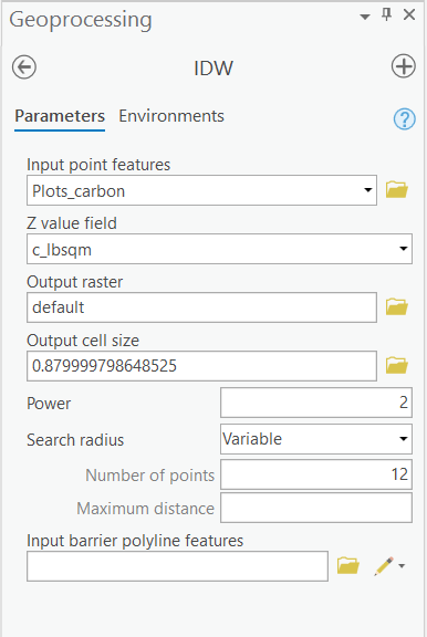
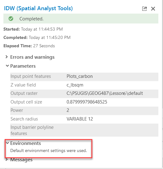
- Within the Analysis tab, go to Tools > Toolboxes > Spatial Analyst Tools > Interpolation > IDW. Use the settings below to interpolate the carbon per square meter values. Save the output raster in your L6Data folder and name it "default." Click Run.
Click the Show Help >> button to help define particular input parameters.
You can review the specific input and environment settings you used in the Analysis tab, Geoprocessing group > History. This can be helpful if you are not sure if you made a mistake somewhere along the way during a complex workflow.
- Change the symbology of the default raster as shown below (5 classes, colors light to dark red).
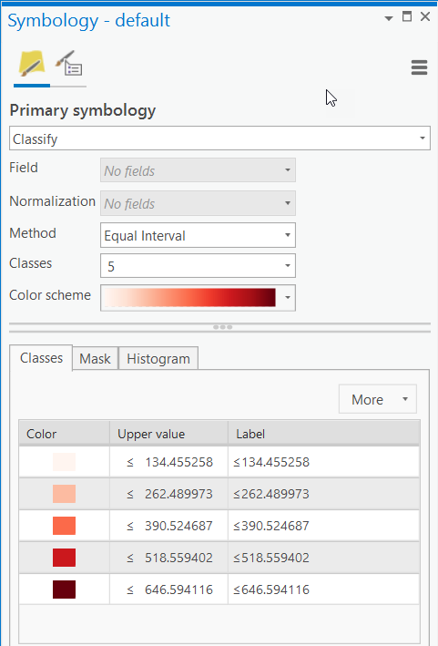
Make sure you have the correct answer before moving on to the next step.
If your map does not match the example below, go back and redo the previous step.
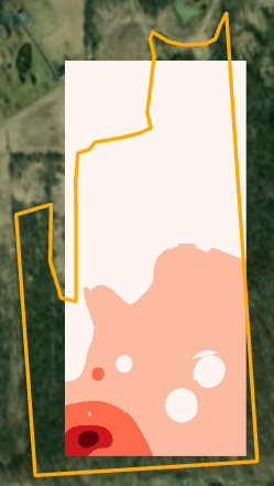
- Compare the results with the "Plots_carbon" shapefile. Areas near plots with high carbon values should be darker than areas near plots with low carbon values. Confirming your output results assures you that you selected the correct input dataset and field to interpolate.
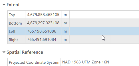
- Notice how the interpolated raster does not match the forest boundary, how the shape of the output grid is a perfect rectangle, how the extent of the raster matches that of the smallest rectangle that can contain all of the plot points, and that the cell size is 0.87999… meters.
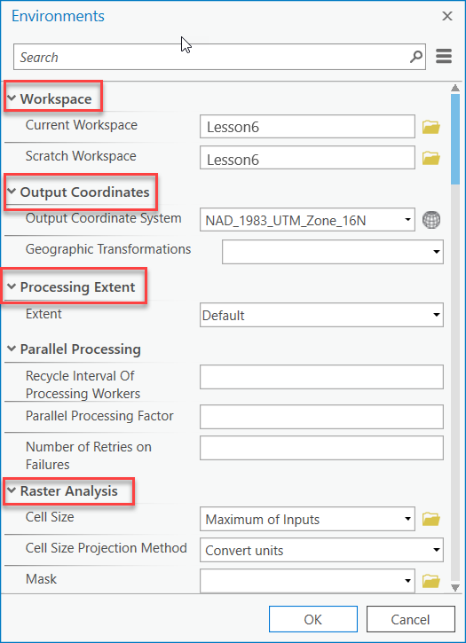
- Why did this occur? Let’s take a look at some of the environment settings utilized by Spatial Analyst to find out. Go to Geoprocessing > Environments. As noted earlier in this course, environment settings are the system-wide default settings that are used by every tool. Spatial Analyst utilizes Workspace, Output Coordinates, Processing Extent, Raster Analysis, and Raster Storage settings.
- Read the embedded help articles for:
- Processing Extent > Extent
- Raster Analysis > Cell Size
- Raster Analysis > Mask
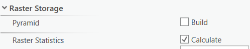
- Raster Storage > Pyramid (scroll down)
- Pyramids allow for the rapid display of large raster datasets at multiple scales. While this may prove useful for very large datasets, creating pyramids has two important drawbacks. First, because of its design, it will generalize data as the scale gets larger, which will reduce the visible accuracy of the displayed data. Second, because of this generalization, layouts created at large scales may not properly represent the actual data, and may appear coarser than it actually is.
- I recommend NOT creating pyramids unless working with a particular dataset significantly degrades the performance of ArcGIS. For this course, we will disable pyramid creation when we set the Spatial Analyst environment settings. To do this, go to Analysis tab, Geoprocessing group, Environments > Raster Storage (scroll down), and uncheck Build. Click OK to save this setting.
What is the default setting for analysis extent?
What is the cell size of the "default" raster we created? Why?
Raster Attribute Tables
You may notice that the option to open the attribute table of the "default" raster is grayed out. ArcGIS Pro only builds raster attribute tables if certain conditions are met. One of the conditions is that the values in the raster have to be integers. Since the values in our raster have decimals, it is not possible to view the attribute table.
- Within the Analysis tab, go to Tools > Toolboxes > Spatial Analyst Tools > Interpolation > IDW. Use the settings below to interpolate the carbon per square meter values. Save the output raster in your L6Data folder and name it "default." Click Run.
-
Interpolate Data – Set Extent
Now that we’ve explored the default settings, let’s see what happens if we alter just the extent settings. Unlike vector files, rasters will always have the shape of a perfect rectangle. The size and location of the rectangle is defined by its extent.
- Within the Analysis tab, Geoprocessing group go to Tools > Toolboxes > Spatial Analyst Tools > Interpolation > IDW.
- Name the output raster C:\GEOG487\L6Data\forest_extent.
- Notice the default cell size is currently listed as 0.879999994163401.
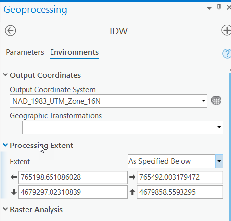
- There is an oddity within ArcGIS where it does not apply all of the global environment settings from the Analysis tab, Geoprocessing group > Environments to some tools within Geoprocessing Toolbox. We’ll need to set the extent settings using the Environments option within the IDW tool itself. Click on Environments > Processing Extent, choose "Same as Layer Forest_Boundary" as the extent.
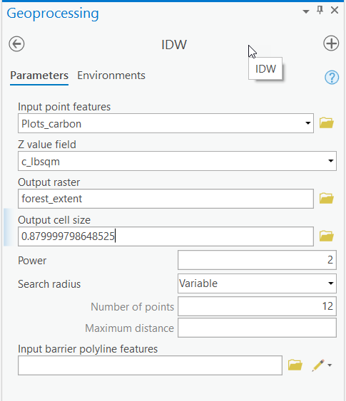
- Notice how the output cell size changed to “1.17340837377682.” Make sure to review the embedded help topic to understand why this happened.
- To keep the output rasters consistent throughout the lesson, we need to manually override the cell size setting in Parameters. Copy and paste 0.879999994163401 into the cell size input and click Run.
Make sure you have the correct answer before moving on to the next step.
If your map does not match the example below, go back and redo the previous step.
- Change the symbology of the forest_extent raster as we did in Step 3b, except use light to dark blue for the color ramp.
- Compare the "forest_extent" raster to the "default" raster. You may need to rearrange the files in the Contents pane. Notice how the extent of the "forest_extent" raster matches that of the smallest rectangle that can contain the forest boundary polygon.
- Repeat Step 4, except use the "Parcel_Boundary" file as the extent. Make sure you use the same cell size as the default and forest-extent rasters. Name the output raster "parcel_extent."
- Change the symbology just as we did previously, except use an orange color scale. Compare the output with the parcel boundary. Save your map.
How do the extents of the "parcel_extent," "forest_extent" and "default" rasters compare?
-
Interpolate Data – Set Mask
Now, let’s see what happens if we alter the mask and extent settings. Even though all rasters are defined as perfect rectangles, you can still represent your data as a sinuous shape. The computer creates this illusion by assigning cells outside the sinuous shape values of "NoData." There is not a direct equivalent to this concept in vector files.
- Within the Analysis tab, Geoprocessing group go to Tools > Toolboxes > Spatial Analyst Tools > Interpolation > IDW.
- Change the output name to “for_msk_ext.”
- Click on Environments > Processing Extent > choose "Same as layer Forest_Boundary" as the extent.
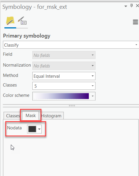
- Within Raster Analysis > select Forest_Boundary as the Mask.
- Make sure the cell size is 0.879999994163401 under the Parameters. Click Run to run the tool.
- Change the symbology as before except use a purple color scale. Compare the output raster to the forest boundary. Your raster should now match the shape and size of the forest boundary polygon.
- What happened to the cells outside of the forest boundary? By default, ArcGIS displays raster values of NoData without a color. Change the color of NoData to black on the symbology tab and examine the results.
-
What would the output raster look like in the following scenario?
- Mask: forest boundary; Extent: parcel boundary
- Mask: parcel boundary; Extent: forest boundary
- Mask: "Plots_carbon" shapefile; Extent: forest boundary
-
Interpolate Data – Set Cell Size
In Step 3, we learned that the default cell size will depend on the input data. If you are using one or more rasters as inputs, the cell size will default to the coarsest raster resolution. If you are using a vector file, it will calculate the cell size based on the extent of the file to create 250 cells. The default for rasters seems appropriate since GIS best practices dictate that you should always go with the cell size of your coarsest input dataset. However, the default for vector files is quite arbitrary.
How do we choose a more meaningful cell size for our analysis? One rule of thumb is that you don’t want to "create" higher resolution data than what exists in your measured values. We know that the tree data was collected by measuring trees that fell within 10 m diameter circular plots. A cell size of 1 cm would not be appropriate, because we do not know how the data varies at that scale. A cell size of 1,000 m would be too large, since it is larger than our study area. For this project, we will use a cell size of 1 m, since our carbon values are in pounds per square meter.
- Within the Analysis tab, Geoprocessing group go to Tools > Toolboxes > Spatial Analyst Tools > Interpolation > IDW.
- Change the output name to "carbon1m."
- Click on Environments to Set the "Forest Boundary" as the mask and extent.
- Change the output cell size to 1. Click Run.
- Change the symbology as before, except use a green color scale. Compare the output to the "for_msk_ext" raster. At first glance, the output raster may not look very much different than the "for_msk_ext" raster, since they have the same mask, extent, and very similar cell size settings.
-
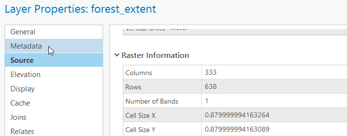
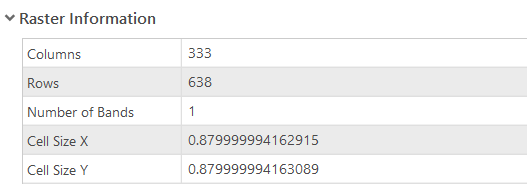
Right-click on the "carbon1m" raster in the Contents pane > Properties > Source. Browse through the available information. Notice the extent and cell size. Compare this information to the properties of the "for_msk_ext" raster as shown on the right.
"carbon1m" properties"for_msk_ext" properties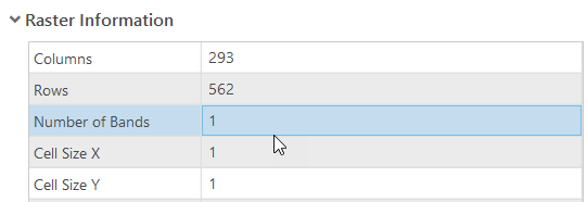
- Interpret Results – Calculate Carbon for Entire Study Area
Now that we have an understanding of how the spatial analyst environment settings function, we can return to our original question. We want to figure out how much carbon the study forest sequesters. To accomplish this, we will use the "Zonal Statistics" tool in Spatial Analyst. This tool allows us to calculate statistics of the cell values of one raster (e.g., carbon1m) within zones specified by another file (e.g., forest boundary). We will use it to sum the carbon values in each cell to create a total for the entire forest.
- Within the Analysis tab, Geoprocessing group go to Tools > Toolboxes > Spatial Analyst Tools > Zonal > Zonal Statistics as Table. Use the settings below to find the total carbon for the forest. Name the output table "carbon1m_sum" in your L6 folder.
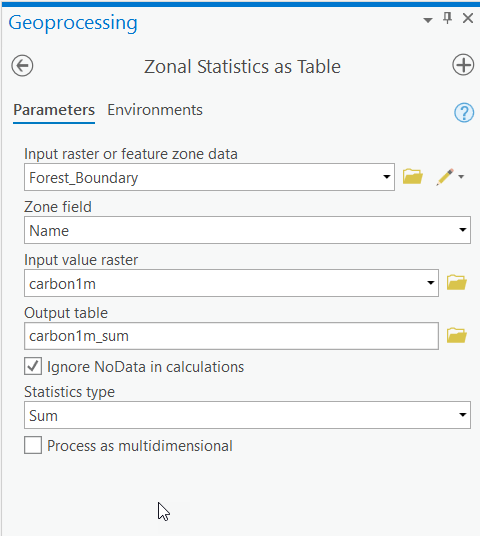
- After you click Run, the summary table will appear in the Contents pane. Right-click to Open the table. Notice the field "SUM." This value represents the total carbon in the forest. Close the table.
- Notice that this table can be joined to the "Forest_Boundary" layer since they share the field "Name". You may find it useful to join these tables together if you wish to visually map the zonal statistics.
ArcGIS may not show all the digits in a table by default. If your numbers do not match the numbers in the quiz, expand the columns in your table to display all the digits.
- One credit is earned for each metric ton (mT) of carbon sequestered. How many carbon credits does the study forest qualify for? Note that 1 metric ton = 2,204.6 lbs.
The monetary value of each carbon credit fluctuates based on the current market conditions. Check out the more information about the California’s cap and trade system at Center for Climate and Energy Solutions(C2ES) [20].
One of the main take away points from this lesson is that Spatial Analyst is a modeling tool. Models don’t give exact final answers; rather they give you estimates of reasonable answers based on a set of assumptions.
Environments settings allow you to easily alter the underlying assumptions of your model (cell size, mask, extent) and then quickly recalculate your results.
Selecting environment settings in Spatial Analyst tools can be confusing and seem somewhat arbitrary. If you don’t know which Environments setting you should use for a particular scenario, you can try experimenting with a variety of options. This type of sensitivity analysis will help you understand how changing model assumptions affect your final results.
That’s it for the required portion of the Lesson 6 Step-by-Step Activity. Please consult the Lesson Checklist for instructions on what to do next.
Try This!
Try one or more of the activities listed below:
- In Lesson 6, we used the defaults for many of the input parameters of the Interpolation Tool such as "z value field," "power," and "search radius type." Alter some of these parameters to see how they affect your results.
- There are several other interpolation methods to choose from in addition to Inverse Distance Weighted, such as "Spline" and "Kriging." Explore some of the other options to see how they affect your results.
- Export the study boundary to a KML file using Toolboxes > Conversion Tools > KML > KML to Layer. Open the KML file in Google Earth, zoom to the study boundary, and explore the historical imagery for the study site.
Note: Try This! Activities are voluntary and are not graded, though I encourage you to complete the activity and share comments about your experience on the lesson discussion board.
- Within the Analysis tab, Geoprocessing group go to Tools > Toolboxes > Spatial Analyst Tools > Zonal > Zonal Statistics as Table. Use the settings below to find the total carbon for the forest. Name the output table "carbon1m_sum" in your L6 folder.
Advanced Activity
Advanced Activity
Advanced Activities are designed to make you apply the skills you learned in this lesson to solve an environmental problem and/or explore additional resources related to lesson topics.
Directions:
After looking at current aerial photos of the site, you realize that the density of tree cover varies across the study area. In fact, there are many parts of the study area that are not covered with trees. Historical aerial photos reveal that the forest is quite young and that many parts of the study area were used for agriculture until quite recently. Using aerial photos from the 1940s to the present, you create a shapefile showing areas of similar age and forest type (Vegetation07.shp in your L6 folder).
Given this new information, you realize that your original estimate of carbon sequestered by the forest is too large since many of the interpolated cells are located within areas that are not covered with trees. You decide to redo your interpolation to remove areas that are not forested from your results. What is your new estimate of carbon sequestered by the study forest?
Summary and Deliverables
Summary and Deliverables
In Lesson 6, we talked about climate change, forests, and carbon credits. We explored how to use GIS to plot and interpolate representative sample data measured in the field. We also explored how altering the extent, mask, and cell size settings within Spatial Analyst lead to very different results. We learned that you need to select settings appropriate for your analysis since accepting the defaults can have unintended consequences. In the next lesson, we will look at two different Spatial Analyst tools: "reclassify" and "tabulate area" to investigate land use change over time.
Lesson 6 Deliverables
Lesson 6 is worth a total of 100 points.
- (100 points) Lesson 6 Quiz
Tell us about it!
If you have anything you'd like to comment on, or add to the lesson materials, feel free to post your thoughts in the Lesson 6 Discussion. For example, what did you have the most trouble with in this lesson? Was there anything useful here that you'd like to try in your own workplace?
Additional Resources
Additional Resources
This page includes links to resources such as additional readings, websites, and videos related to the lesson concepts. Feel free to explore these on your own. If you would like to suggest other resources for this list please send the instructor an email.
Websites:
- REDD+ Reducing Emissions from Deforestation and Forest Degradation [21]
- United Nations Framework Convention on Climate Change [22]
- Intergovernmental Panel on Climate Change (IPCC) [23]
- IPCC Assessment Reports [24]
- U.S Forest Service Climate Change Resource Center [25]
- United Nations Carbon Offset Platform [26]
- Green Climate Fund [27]
- National Tree Benefit Calculator [28]
Articles & Reports:
- Measuring tree diameter to calculate aboveground forest carbon at Penn State's Stone Valley Experimental Forest [29]
- Mapping the irrecoverable carbon in Earth’s ecosystems [30]
- Findings of the Intergovernmental Panel on Climate Change "Report on Climate Change Impacts Part II" [31]
- "Deforestation Success Stories: Tropical Nations Where Forest Protection and Reforestation Policies Have Worked" [32]
- "Mapping the potential for REDD+ to deliver biodiversity conservation in Viet Nam" [33]
- Congressional Reserach Service "Reduction in Emissions from Deforestation and Forest Degradation (REDD+)" [34]