Lesson 7: The Role of Forests
Lesson 7 Overview and Checklist
Lesson 7 Overview
Scenario
You have been hired by a conservation group to determine how selective logging practices have changed a rainforested area in the Congo Basin of Central Africa. You must use ArcGIS and Spatial Analyst to determine the number of forest fragments that have been created by logging roads. You also need to characterize the habitat quality of each forest fragment in terms of the ratio of interior to edge habitat, the edge to area ratio, the thickness, and the overall area.
Goals
At the successful completion of Lesson 7, you will have:
- converted vector data to raster data using Spatial Analyst;
- created raster regions using Spatial Analyst;
- calculated thickness, area, and perimeter of raster regions;
- shared analysis results created in ArcGIS using ArcGIS Online.
 |
 |
 |
 |
 |
Questions?
If you have questions now or at any point during this lesson, please feel free to post them to the Lesson 7 Discussion.
Checklist
This lesson is one week in length and is worth a total of 100 points. Please refer to the Course Calendar for specific time frames and due dates. To finish this lesson, you must complete the activities listed below. You may find it useful to print this page out first so that you can follow along with the directions. Simply click the arrow to navigate through the lesson and complete the activities in the order that they are displayed.
- Read all of the pages listed under the Lesson 7 Module.
Read the information on the "Background Information," "Required Readings," "Lesson Data," "Step-by-Step Activity," "Advanced Activities," and "Summary and Deliverables" pages. - Read and watch the required readings and videos.
See the "Required Readings and Videos" page for links. - Download Lesson 7 datasets.
See the "Lesson Data" page. - Download and complete the Lesson 7 Step-by-Step Activity.
- See the "Step-by-Step Activity" page for a link to a printable PDF of steps to follow.
- Complete the Lesson 7 Advanced Activity.
See the "Advanced Activity" page. - Complete the Lesson 7 Quiz.
See the "Summary and Deliverables" page. - Create and post links to Lesson 7 Maps and App.
Specific instructions are included on the "Summary and Deliverables" page. - Optional - Check out additional resources.
See the "Additional Resources" page. This section includes links to several types of resources if you are interested in learning more about environmental data covered in this lesson.
SDG image retrieved from the United Nations [1]
Background Information
Background Information
Logging in Tropical Rainforests
Tropical rainforests are extremely valuable in terms of the ecological services they provide, such as biodiversity and carbon sequestration. Although they cover only 6% of the earth's surface, they provide habitat for over half of the plants and animals in the world. Many of these plants and animals are threatened or endangered species. Rainforests are also highly prized for their commercial hardwood trees. The trees are cut down and processed to create products such as teak and mahogany furniture, plywood, and flooring.
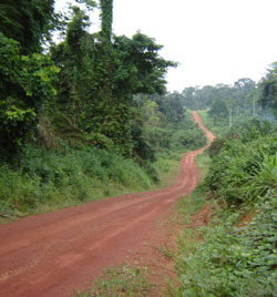
Historically, there are two main types of logging practices used in tropical forests: clearcutting, and selective logging. During clearcutting, loggers remove all of the trees in a given area, leaving large clearings in their wake. These clearings reduce the amount of usable habitat for plants and animals. You can view an example of clearcutting in Brazil by looking in Google Maps [2]. Notice the large grey patches in the images. These are areas of the forests that were cleared of all vegetation. Without vegetation to stabilize the soil, winds, and rain quickly erode the nutrient-rich soils required for new species to colonize the area. Clearcutting is a very environmentally destructive process. While on Google Maps, be sure to zoom out a little, and you will see the fishbone pattern that is characteristic of logging in tropical forests. Also, check out the article "Roads could help protect the environment rather than destroy it, argues Nature Paper [3]."
In contrast, only species of value are extracted from the forest during selective logging. It seems like this process would be much more environmentally friendly, considering that much of the logged area remains forested. However, it is also a destructive process because it opens up previously inaccessible areas to human exploitation, damage, and degradation. Once logging roads are built, they tend to be used for many other activities. For example, bushmeat hunters use new roads to extract and transport illegal forest products such as monkeys, gorillas, and chimpanzees. Migrating people often travel along these roads and establish new villages. Once settled, they tend to clear surrounding areas of the forest for agriculture using slash-and-burn techniques.
Forest Fragmentation and Edge Effects
As loggers build new roads, they break up large tracts of forest into progressively smaller areas or “patches.” This process is known as "forest fragmentation." Scientists use a quantity called the "edge to area ratio" to characterize forest fragments. The measurement, calculated as the perimeter of forest/area of forest, represents the complexity of the shape of each forest patch. The higher the value, the more irregular the forest boundary.
In addition to breaking up forests into smaller patches, road building activities also increase disturbances known as "edge effects." Some examples of edge effects include changes in species composition, diversity, and seed dispersion, increased tree mortality and susceptibility to fires, microclimate shifts (humidity and sunlight), increased carbon emissions, and impeding movement of animals. Scientists have observed edge effects up to 2 km from road edges.
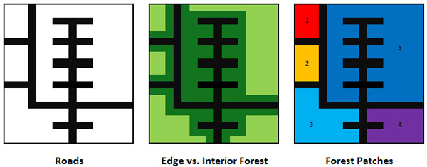
Logging activities can have a significant impact on the local ecosystem since the smaller forest patches do not provide the same quantity and quality of habitat as large tracts. As new roads are built, fragments of forests are further degraded as the ratio of interior habitat to edge habitat decreases. Native animal species of tropical rainforests can require blocks of interior habitat greater than 1,000 sq km. Large mammals and species under hunting pressure can require interior areas of at least 10,000 sq km. To create large areas of interior habitat, care must be taken to limit road building activities to certain areas.
Study Area
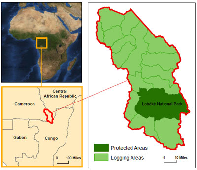
In Lesson 7, we are going to examine the effects of historical commercial logging activities for a forested area in southeastern Cameroon. The study area is part of the Congo Basin, which contains the world's second-largest concentration of tropical rainforests. The study area boundary encompasses two main types of land management areas: protected areas and logging areas. The Lobeke National Park is the main protected area within the study site. Using GIS datasets showing road centerlines, we will use ArcGIS Spatial Analyst to quantify the fragmentation and edge effects within the study area.
Required Readings & Videos
Required Readings & Videos
There are three types of required readings for Lesson 7: a short video describing issues facing forests and the conservation group - World Resources Institute (WRI) that created the data we will use in the lesson, background information about the study area, and Esri Help Topics related to the GIS tools we will use in the lesson.
Video: WRI's Forest Team - Part I (9:54)
Note: If you do not see the embedded video below, try clicking the refresh button on your browser, try viewing this page in another browser, or click on the hyperlink listed as the source.
This is a water filtration system.
This is an air purifier.
This is food and shelter.
This is building material and paper.
This is a pharmacy.
This is fuel to millions of people around the world.
This is a climate regulator.
This is a forest.
I'm Jonathan Lash. I'm the president of the World Resources Institute and I'd like to talk with you about forests. It's very likely that the breakfast table you sat at this morning was made with wood from a forest you've never met. In fact, probably the coffee you drank used water and coffee that came or were affected by a forest somewhere on earth. In light of all the things that forests do for us, it's actually quite astonishing how little good information there is about forests worldwide, and the forces affecting them. That's why my colleagues work with partners in every forested country to provide better information to governments, to non-governmental organizations, and to businesses, to enable better decisions about the future of forests. I hope you'll enjoy meeting some of my colleagues and hearing about what they do.
WRI’s global network has mapped all of the world's intact forest landscapes. Companies, governments, and environmental groups use our maps and expertise to balance conservation and development needs.
We train our partners on how to use computer-based information to help them make better decisions about forest management.
We help decision-makers address complex interconnected issues, such as climate change and deforestation.
We provide buyers with reliable, impartial, and easy-to-understand advice and sustainable procurement of forest products.
We build partnerships among timber companies, governments, training institutions, civil society organizations, and local populations. This ensures that our partners buy in and use our information tools.
At the dawn of Agriculture, almost half of the planet's land surface was covered by vast tracks of forest. Since then, almost half of those forests have been lost. Today, five large intact forest landscapes remain. They are the Boreal forests of Russia and Canada and the tropical forests of Southeast Asia, Central Africa, and the Amazon basin. Some of these forests are under tremendous pressure. From agricultural and timber industry expansion to illegal logging and lack of accountability, all can lead to these intricate landscapes being degraded or disappearing entirely.
To manage forests, you need recent and reliable information. WRI creates maps with accurate and up-to-date data. These maps show where the forests are and where deforestation is occurring. They allow decision-makers to analyze decreasing forest areas and figure out how to better manage their forests.
Let us take you on four brief trips to Russia, South America, Central Africa, and Indonesia and show you what we do.
In Russia, our maps have helped the negotiation and conflict resolution. WRI and our partners created a detailed forestry atlas of high conservation value forest in the Russian Far East. This atlas makes it possible to see both the Russian government's forest quadrants and the high conservation value forest on the same map. The atlas helped settle an impasse between a big Russian timber company called Turnalias and a group of Russian and international NGOs. At issue was Turnalias’ activity in a hitherto untouched river basin. Once both parties had access to an accurate and detailed map, they were able to negotiate meaningfully and reach a lasting compromise solution. Turnalias agreed to keep a moratorium on logging and road construction in the higher conservation value areas. They further agreed to support working with the NGOs to survey the areas and decide which would become protected areas and which would be opened up to logging.
WRI maps are guiding forest companies doing business in boreal forest regions across Russia and Canada. The Forest Stewardship Council, one of the globally recognized labels for sustainable forest management, also uses WRI Maps. FSC ensures that timber companies seeking to be certified take proper account of large forests of high conservation value.
The Amazon is a precious natural resource subject to significant human pressures. For successful forest management and conservation, it is critical to identify these pressures and understand how they are related. Two major pressures on forests are agriculture and ranching, but to get a more complete picture WRI and a Brazilian organization, Amazon, identified additional factors, such as settlements, fires, and mining. Together they mapped these pressures across the Brazilian Amazon. This map provided critical data to the Brazilian government and informed the government's decisions about where to establish new federally and state protected areas, leading to the protection of over 16 and a half million hectares of important rainforest.
After the Amazon, the Congo Basin of Central Africa contains the second-largest block of a moist tropical forest in the world. But lack of information, limited government capacity, and weak governance have led to poor forest management. WRI is working with governments in the region to address these issues and to help improve the management of forest resources in central Africa. In central Africa, until recently, forest information was paper-based and scattered throughout various government ministries in each country. The result was a lack of standardized data and sometimes even led to conflicting information. Gathering all of the information in one standardized geographic information system or GIS database, to produce up-to-date forestry maps and interactive atlases, was WRI’s first step to improve the accuracy, completeness, and quality of the forest information. To do this, WRI set up in-country GIS laboratories and partnered with these countries' governments and local NGOs to digitize maps of all recognized logging titles and protected areas. Working with local partners, WRI was able to clean up overlapping boundaries and fill in the missing information. We also trained our partners on how to use satellite images to pinpoint when and where logging activity was occurring. The government ministries in charge of forests in central Africa now use these atlases to monitor activities in the country's forests and better manage logging concessions. With a single harmonized set of digital forest data, the forest ministries avoid past mix-ups between agencies and local NGOs are now able to more effectively monitor ongoing activity. These atlases are proving to be powerful tools for fighting illegal logging.
Indonesia has one of the world's highest deforestation rates. WRI’s fire maps and interactive atlases are now helping Indonesia and other countries address climate change. Large intact forest landscapes, such as those in Indonesia, are vital to keeping the world's climate in balance. But the clearing and burning of primary forests and peatlands, much of it for new oil palm plantations, has made Indonesia one of the highest emitters of greenhouse gases in the world.
The international community is developing a mechanism to combat climate change through better forest management, called RED, which stands for Reduced Emissions from Deforestation and Forest Degradation, in developing countries. Through RED, industrialized countries that cannot reduce their carbon emissions to target levels would pay developing countries to keep their forests intact. WRI partnered with Indonesia's Ministry of Forestry, the World Bank, local NGOs, and remote sensing experts, to analyze the carbon content of Indonesia's forests. This unique forest monitoring system helps equip the Indonesian government with the credible information it needs to enter into international negotiations on RED.
Study Area Information:
- Description of the Lobeke National Park - "Mapping Suitable Great Ape Habitat in Lobéké National Park, South-East Cameroon [4]".
Esri Help Topics
Find the help articles listed below in the ArcGIS Pro Resources Center [5].
Search for:
- "Converting Features to Raster Data [6]"
- "An Overview of the From Raster toolset [7]"
- "An Overview of the To Raster toolset [8]"
- "Mosaic To New Raster (Data Management) [9]"
- "How Raster Calculator works [10]"
- "Histogram [11]"
- "Zonal Histogram (Spatial Analyst) [12]"
- "Region Group (Spatial Analyst) [13]"
- "How Zonal Geometry works [14]"
Lesson Data
Lesson Data
This section provides links to download the Lesson 7 data along with reference information about each dataset (metadata). Briefly review the information below so you have a general idea of the data we will use in this lesson.
Lesson 7 Data Download:
Note: You should not complete this activity until you have read through all of the pages in Lesson 7. See the Lesson 7 Checklist for further information.
Create a new folder in your GEOG487 folder called "Lesson7." Download a zip file of the Lesson 
Metadata
Publicly Available Data:
Base Map:
- Source: Esri Basemap
- Service Names: Imagery Hybrid
- Within ArcGIS, go to the Map tab within the Layer group and click on the Basemap (select Imagery Hybrid from the dropdown menu).
Private Data (Located Inside the Lesson7 Data Folder):
The data for this lesson is contained in a geodatabase called Lesson7.gdb. Read about geodatabases in the online help provided by Esri if you are not familiar with this data format.
- Study_Boundary: The study site is located in Southeastern Cameroon.
- Management Units: Encompasses land management units designated for conservation and logging.
- Roads07: Road centerlines digitized from 2007 Landsat images.
- Roads01: Road centerlines digitized from 2001 Landsat images.
- Roads21: Road centerlines sourced from 2021 Landsat images and OpenStreetMap
The roads and study boundary were sourced from portions of the Interactive Forestry Atlas [16], Global Forest Watch Open Data Portal [17], Humanitarian Data Exchange [18], and OpenStreetMap [19] for our study area. The original data was created by the World Resources Institute - Global Forest Watch [20] (GWF), a nongovernmental organization (NGO) focused on environmental issues. They regularly produce reports and data about the state of forests and logging in Central Africa and other locations around the world. Part of their work involves the creation of GIS datasets to assist forest managers.
Step-by-Step Activity
Step-by-Step Activity: Overview
Step-by-Step Activity: Overview
In Part I, we will review the historical data and organize the map for analysis. In Part II, we will use the roads dataset to create rasters of habitat quality and forest patches. In Part III, we will generate statistics about the size, shape, and habitat quality of each forest patch. We will also generate statistics of habitat quality by land management type (conservation vs. logging areas). In Part IV, we will share our analysis results using ArcGIS Online.
Lesson 7 Step-by-Step Activity Download
Note: You should not complete this step until you have read through all of the pages under the Lesson 7 Module. See the Lesson 7 Checklist for further information.
Part I: Review the Relevant Data Layers and Organize the Map
Part I: Review the Relevant Data Layers and Organize the Map
In Part I, we will review the data and organize the map for analysis.
-
Unzip the Data for Use in ArcGIS
- Unzip the Lesson 7 data in your L7 folder. Since all of the data is included in this zip file, you do not need to worry about how you unzip the data.
- Familiarize yourself with the contents of the data included in this zip file. Refer to the Lesson Data section for additional information.
-
Organize the Map and Familiarize Yourself with the Study Area
Since all of the datasets used in this lesson have the same projection, we do not have to be concerned with the order in which we load the data.
- Start ArcGIS and create a new blank map and save the project in your Lesson7 folder.
- Add the "Study_Boundary," "Management_Units," and "Roads07" feature classes from the "L7Data.gdb" geodatabase located in your L7Data folder.
- Change the symbology of the layers as follows: Study_Boundary – hollow red line; Management_Units – unique values by ‘Use’; Roads07 – black line.
- Rearrange the layers so the study area boundary is on top and the roads are on the bottom.
- Explore the attribute tables of the three feature classes.
- Update your Environments: workspaces should be the L7 folder, and the output coordinates, mask, and extent should be the same as layer "Study_Boundary," the cell size to 100 meters, and uncheck the “Build Pyramids” box.
- Add the "Imagery Hybrid" ArcGIS Basemap to your map and drag it below the boundaries. Notice the location of the study boundary in relation to the country of Cameroon and the Congo Basin.
- Save your project. You may want to turn off the basemap if you experience any slow-down during the lesson.

How many of the management units are used for logging? What about conservation?
Using the "Imagery Hybrid" layer, can you see the approximate extent of the rainforests located in the Congo Basin? What kind of details can you see in the forest if you zoom in very close?
Part II: Create Habitat Quality and Forest Patch Datasets
Part II: Create Habitat Quality and Forest Patch Datasets
In Part II, we will use the roads dataset to create raster data layers of habitat quality and forest patches. In Part III, we will generate statistics about the size, shape, and habitat quality of each forest patch.
We will use the following coded values:
- 1- Low Quality Habitat (Road Clearings)
- 2- Medium Quality Habitat (Forest, Edge Habitat)
- 3- High Quality Habitat (Forest, Interior Habitat)
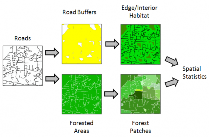 Road Dataset Flow ChartClick here for an accessible text alternative to the image aboveRoads → Road Buffers → Edge/Interior Habitat → Spacial Statistics Roads → Forested Areas → Forest Patches → Spacial Statistics
-
Create Grid of Low-Quality Habitat (Road Clearings)
- Open the "Roads07" attribute table and add a new short integer field named "HabitatCode." Save your changes.
- Use the Calculate Field tool to assign all of the roads a HabitatCode of "1." Clear the selected records.

When you convert a feature layer to a raster, you have to choose a field in the feature layer from which to base the grid cell values on. You often need to create a new dummy field and assign a value that is consistent for all of the records you want to convert (like we did above).
It is also important to note that if there are any selected records in the vector layer, only those records will be converted to a raster layer. Therefore, be sure to clear any selected features before performing the conversion.
The data type of the field you choose is very important. For example, if you choose a numerical field that contains decimal values, the resultant grid will not have an attribute table. However, if you choose an integer field, the resultant raster will have an attribute table. If you choose a text field, ArcGIS will automatically assign each unique text value an integer code in a new field named "VALUE."
The new raster layer will be created based on all defined Spatial Analyst environment settings. Always check these settings before converting features to a raster to avoid potentially undesirable results.
- Convert the roads feature class to a raster named "RoadsGrid.tif" using the settings below: Analysis > Tools > Toolboxes > Conversion Tools > To Raster > Feature to Raster.
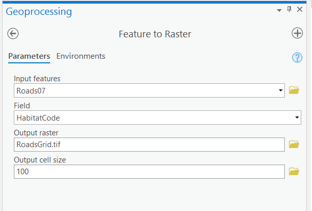
- Click Run. Compare the "RoadsGrid.tif" to the road centerlines. Make sure you zoom to several different scales. Open the "RoadsGrid.tif" attribute table to view the results.
It is important to note that although the extent setting is utilized by Feature to Raster, the mask setting is ignored. Although you will not notice this with the "RoadsGrid.tif" layer, you will see the effects of this when you create a buffered grid later in this lesson.

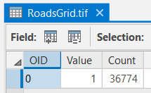
Make sure you have the correct answer before moving on to the next step.
The "RoadsGrid.tif" raster should have the following information. If your data does not match this, go back and redo the previous step.
-
Create Edge Effects Grid
Remember from the Background Information section that edge effects can occur up to 2 km from roads. We will consider all areas 2 km from roads as "edge habitat" and areas farther than 2 km from roads as "interior habitat." To do this, we need to create a buffer of the road centerlines.
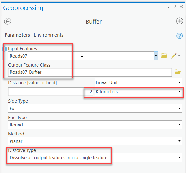
- Create a 2 km buffer of the road centerlines. Go to the Analysis tab, within the Tools group and click Buffer
 . Using the settings specified in red boxes below (allow other settings to default). Save the file inside the Lesson 7 geodatabase.
Click Run.
. Using the settings specified in red boxes below (allow other settings to default). Save the file inside the Lesson 7 geodatabase.
Click Run.
- Compare the buffer to the road centerlines. You may want to use the measuring tool to double check your buffer is the correct width.
- Add a new short integer field named "HabCode" to the "Roads07_Buffer" feature class and assign it a value of "2" using the field calculator. The value of "2" corresponds to medium quality habitat (forested areas within 2 km of a road).
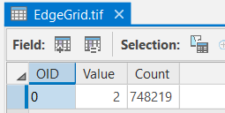
- Convert the road buffer to a grid named "EdgeGrid.tif" based on the "HabCode" field. Be sure to pay attention to the cell size.
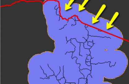
- Compare the "EdgeGrid.tif raster to the "Roads07" and "Roads07_Buffer" datasets. Notice how the conversion tool did not follow the mask setting, as the raster cells with values extrude beyond the study area boundary. It may be easier to see the effect if you assign values of NoData in the EdgeGrid raster a color as we did in previous lessons.
Make sure you have the correct answer before moving on to the next step.
The "EdgeGrid" raster should have the following information. If your data does not match this, go back and redo the previous step.
- Create a 2 km buffer of the road centerlines. Go to the Analysis tab, within the Tools group and click Buffer
-
Create Interior Forests Grid
- Open the "Study_Boundary" attribute table and add a new short integer field named "Value." Save your changes.
- Use the Calculate Field tool to assign a Value of "1" to the study boundary.
- Convert the Study_Boundary feature class to a raster named "Study_Boundary.tif" using the Value field and an output cell size of 100: Analysis > Tools > Toolboxes > Conversion Tools > To Raster > Feature to Raster.
- Reclassify the "EdgeGrid.tif" and use the "Study_Boundary.tif" as the mask. See the other settings below. Name the output grid "InteriorGrid.tif" and click Run.
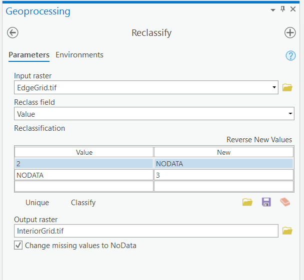
- Compare the "InteriorGrid.tif" raster layer to the "EdgeGrid.tif" and "RoadsGrid.tif" layers. Notice how we were able to "flip" the areas with NoData. It is easier to see the effect if you turn off all of the layers except the Roads, InteriorGrid, and Study Boundary. It’s important that you choose appropriate mask and extent settings when using this technique.
Did the Reclassify Tool honor the mask and extent settings?
Hint: Compare the InteriorGrid.tif and EdgeGrid.tif rasters along the study area boundary.
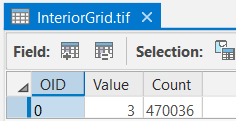
Make sure you have the correct answer before moving on to the next step.
The "InteriorGrid.tif" grid should have the following information. If your data does not match this, go back and redo the previous step.
-
Create Final Habitat Quality Grid
In steps 1, 2, and 3, we created three individual grids, one for each level of habitat quality. To continue the analysis, we need a way to merge all of the data sets into one grid. The Mosaic to New Raster tool in Toolboxes will allow you to mosaic multiple raster data layers together by stacking them on top of one another. The values in the output raster will be determined based on the order the files are specified during the mosaic. Cells will first be assigned according to the cell values in the first input raster; all remaining null values will be filled in with the middle input raster, and so on. We want the roads to be on top of the stack, the edge habitat in the middle, and the forests on the bottom.
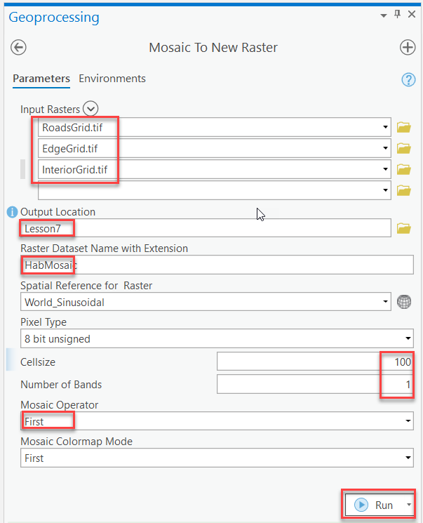
- Go to the Analysis tab, Geoprocessing group and select Tools > Toolboxes > Data Management Tools > Raster > Raster Dataset > Mosaic to New Raster and enter the settings as shown below. Name the new grid "HabMosaic" and save it to your L7 folder. When adding the input rasters, pay attention to the order in which you add them. Along with the output location and the raster dataset name, you will need to assign a cell size and number of bands. The number of bands refers to a color map. Since we are not dealing with multiple band data, enter "1" to identify the new raster dataset as a single band layer. As mentioned above, we want the raster to be created based on a hierarchy from first to last. Therefore, we need to set the Mosaic Operator to "FIRST" so that the analysis runs as intended. You can leave the Mosiac Colormap Mode setting to "FIRST" since we are dealing with single-band data.
This tool does not honor the Output extent environment settings. If you want a specific extent for your output raster, consider using the Clip tool. You can either clip the input rasters prior to using this tool, or clip the output of this tool.
Make sure you have the correct answer before moving on to the next step.
The "HabMosaic" raster should have the following information. If your data does not match this, go back and redo the previous step.
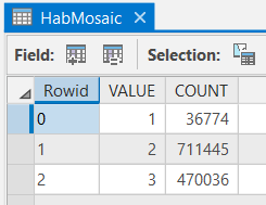
What value was assigned to areas with roads, since they have data in both the "RoadsGrid" and "EdgeGrid" rasters?
Which habitat type (roads, edge, or interior) covers the majority of the study area?
How can you calculate the area of each habitat type?
- Notice that some edges of the "HabMosaic" grid fall outside of the study boundary. As mentioned earlier, this is because the Mosaic to New Raster tool does not utilize the environments extent setting. Therefore, we need to "clip" the data to the extent of our study boundary. To do this, we will use the Raster Calculator. Open the Raster Calculator (Toolboxes > Spatial Analyst Tools > Map Algebra > Raster Calculator), click the "HabMosaic" grid to enter it into the expression window, set the output raster as "HabitatGrid" and click OK to run the expression.
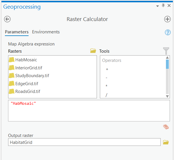
- Compare the "HabitatGrid" to the "HabMosaic" grids to see how the Raster Calculator "clipped" the data. Hint: Zoom into the study area boundary,
The Raster Calculator utilizes all raster environment settings, so it is highly useful when working with raster data. As displayed above, simply selecting a raster layer and running the Raster Calculator will generate a new raster layer based on the current environmental settings. Try changing these settings to see the differences when running the Raster Calculator on a particular raster layer.
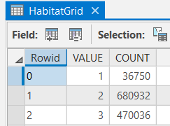
Make sure you have the correct answer before moving on to the next step.
The "HabitatGrid" raster should have the following information. If your data does not match this, go back and redo the previous step.
- Go to the Analysis tab, Geoprocessing group and select Tools > Toolboxes > Data Management Tools > Raster > Raster Dataset > Mosaic to New Raster and enter the settings as shown below. Name the new grid "HabMosaic" and save it to your L7 folder. When adding the input rasters, pay attention to the order in which you add them. Along with the output location and the raster dataset name, you will need to assign a cell size and number of bands. The number of bands refers to a color map. Since we are not dealing with multiple band data, enter "1" to identify the new raster dataset as a single band layer. As mentioned above, we want the raster to be created based on a hierarchy from first to last. Therefore, we need to set the Mosaic Operator to "FIRST" so that the analysis runs as intended. You can leave the Mosiac Colormap Mode setting to "FIRST" since we are dealing with single-band data.
-
Create Grid of Forested Areas
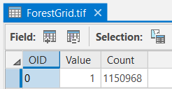
We now have one grid with values showing the range of habitat quality within the study area. The next step is to create a grid of forested areas, which we need to create the forest fragments. We will use the "RoadsGrid.tif" raster we created in Part II Step 1 to create a new grid representing forested areas (cells that are NOT roads).
- Reclassify "RoadsGrid.tif" using the settings below:
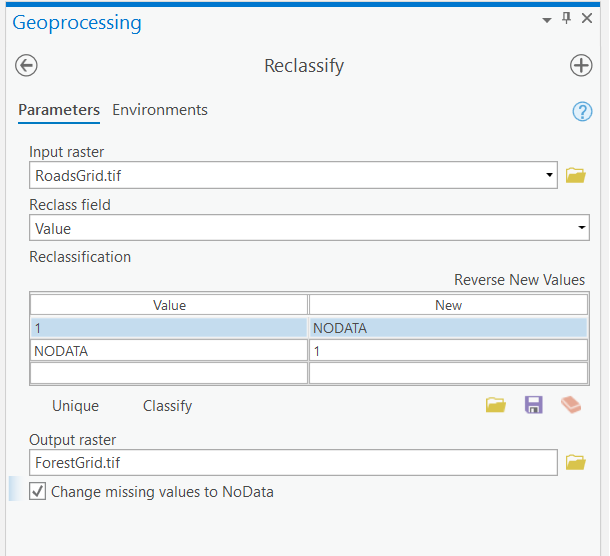
- Compare the "ForestGrid.tif" raster to the "RoadsGrid.tif" raster.
Make sure you have the correct answer before moving on to the next step.
The "ForestGrid.tif" raster should have the following information. If your data does not match this, go back and redo the previous step. You may need to adjust for the Mask and Processing Extent here as well.
- Reclassify "RoadsGrid.tif" using the settings below:
-
Create Grid of Individual Forest Patches
- Examine the "ForestGrid.tif" attribute table. Notice there is not a way to distinguish groups of contiguous cells from one another. We need to be able to do this to determine which cells belong to the same forest patch.
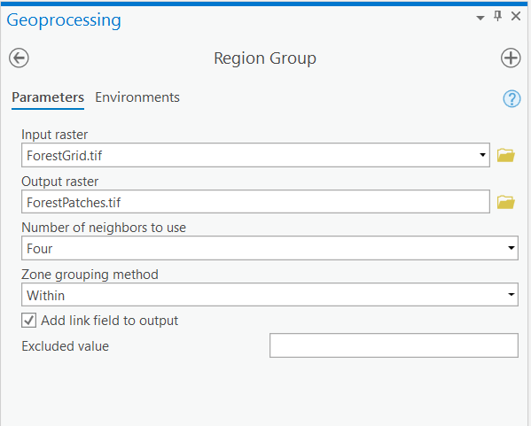
- To accomplish this, we will use the RegionGroup tool. RegionGroup is an operation that takes adjacent cells with the same value and assigns them a unique value. So, in essence, it creates a grid with groups of cells similar to polygons in a feature class layer. This is an important operation since it enables further analysis with expressions and operations that require grouped regions, such as calculating the area and width of forest patches.
- Go to Toolboxes > Spatial Analyst Tools > Generalization > Region Group, select "ForestGrid.tif" as the input raster, name the output raster "ForestPatches.tif", leave the number of neighbors to use as "FOUR", the zone grouping method as "WITHIN", leave the link and excluded value setting, and click Run.
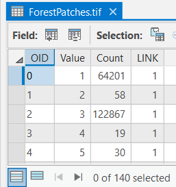
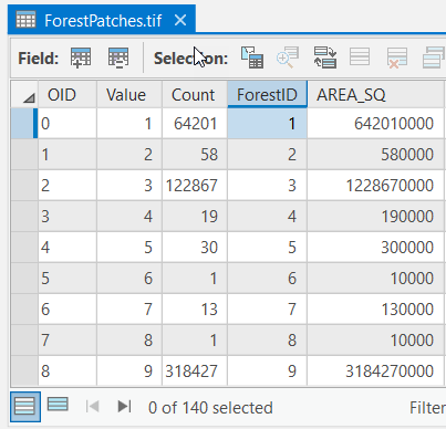
- Compare the ForestPatches.tif attribute table to the ForestGrid.tif attribute table. Notice how the attribute table now has multiple rows, one for each forest patch. The "Rowid" and "VALUE" fields both contain unique ID numbers for each contiguous forest patch. The "COUNT" field shows the number of cells in each forest patch.
Make sure you have the correct answer before moving on to the next step.
The "ForestPatches.tif" grid should have the following information. If your data does not match this, go back and redo the previous step.
 Click here for an accessible version of the image above
Data to Compare your results to OID Value Count link 0 1 64201 1 1 2 58 1 2 3 122867 1 3 4 19 1 4 5 30 1 - The "VALUE" field is very important since it uniquely identifies each forest patch. However, the default name assigned by the computer is not very meaningful. It would be very easy to forget what it means later on. It’s also easy to confuse the "VALUE" and "Rowid" field since they contain similar numbers.
- To prevent these issues, let’s create a more meaningful attribute to keep track of the forest patches. Add a new short integer field named "ForestID" to the "ForestPatches.tif" attribute table. Populate it with the numbers in the !VALUE! field.
- Change the symbology to "unique values" based on the "ForestID" field. Notice how groups of contiguous cells are now considered one unit. Also, notice how the default colors assigned by ArcGIS are not very meaningful. We will address this later in the lesson.
- The "COUNT" field is also very important since it tells us how many cells are within each forest patch. As we saw in Lesson 5, we can use the number of cells and the size of each cell to calculate area values.
- Add a new float field to the "ForestPatches.tif" attribute table named "AREA_SQM." Use the calculate field tool to populate the field.
You can also delete the Link field.
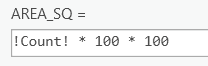
Why did we use the number "100" to calculate the area?
Make sure you have the correct answer before moving on to the next step.
The "ForestPatches.tif" grid should have the following information. If your data does not match this, go back and redo the previous step.
 Click here for an accessible version of the image above
Data Values to Compare To oid value count forestid area_sq 0 1 64201 1 642010000 1 2 58 2 580000 2 3 122867 3 1228670000 3 4 19 4 190000 4 5 30 5 300000 5 6 1 6 10000 6 7 13 7 130000 7 8 1 8 10000 8 9 318427 9 3184270000 How many individual forest patches are there? Which forest patch is the largest? Which forest patch is the smallest? Why do you think there are so many patches with an area of exactly 10,000 sq m?
Part III: Calculate Spatial Statistics of Forest Patches
Part III: Calculate Spatial Statistics of Forest Patches
In Part III, we will use two Spatial Analyst tools to bring together the raster layers we created in Part I (habitat quality) and Part II (forest patches). Zonal Geometry calculates several geometry measures, such as area and thickness, for zones in a raster. We will use it to generate a table of statistics about the size and shape of each forest patch. We will also use the Zonal Histogram Tool to tabulate the number of cells of each habitat type within each forest patch and management unit.
-
Calculate the Geometry of Each Forest Patch
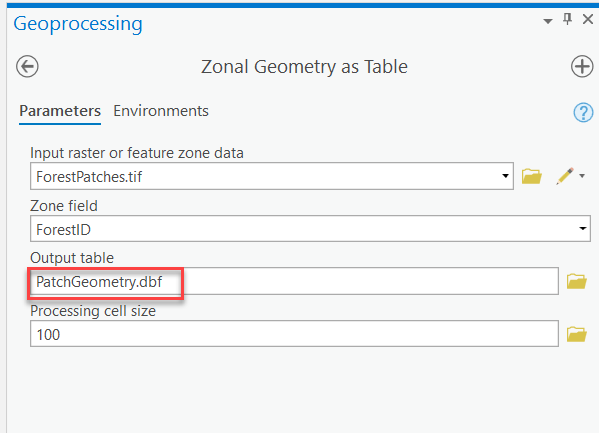
- Go to Toolboxes > Spatial Analyst Tools > Zonal > Zonal Geometry as Table. Use the settings shown below. Name the table "PatchGeometry.dbf" and save it in your Lesson7 folder. Make sure to include the .dbf file extension.
Make sure you have the correct answer before moving on to the next step.
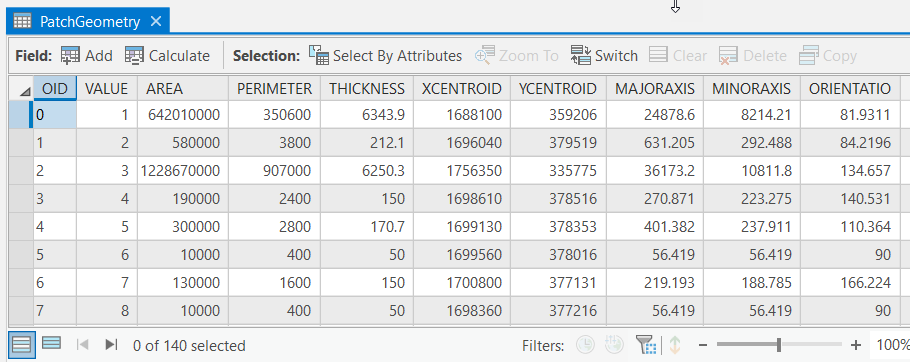
The "PatchGeometry" table should have the following information. If your data does not match this, go back and redo the previous step.
 Click here for an accessible alternative to the image above
Accessible PatchGeometry Data Set OID Value Area Perimeter Thickness Xcentroid ycentroid Majoraxis minoraxis orientation 0 1 642010000 350600 6343.9 1688100 359206 24878.6 8214.21 81.9311 1 2 580000 3800 212.1 1696040 379519 631.205 292.488 84.2196 2 3 1228670000 907000 6250.3 1756350 335775 36173.2 10811.8 134.675 3 4 190000 2400 150 1698610 378516 270.871 223.275 140.531 4 5 300000 2800 170.7 1699130 378353 401.382 237.911 110.363 5 6 10000 400 50 1699560 378016 56.419 56.419 90 6 7 130000 1600 150 1700800 377131 219.193 188.785 166.224 7 8 10000 400 50 1698360 377216 56.419 56.419 90 Which field in the "PatchGeometry" table is the equivalent to the "ForestID" field? What are the units of the fields "AREA," "PERIMETER," and "THICKNESS"? What do the values in the fields "XCENTROID," "YCENTROID," "MAJORAXIS," "MINORAXIS", and "ORIENTATION" mean?
- Add a new short integer field named "ForestID" and populate it with the values in the "VALUE" field using the field calculator. This step will make it easier to compare the Patch Geometry table with other outputs later in the lesson.
- Add three new float fields named “TotAreaSQM,” “PerimeterM", and “ThicknessM.” Calculate them to equal the values in “AREA,” "PERIMETER,” and "THICKNESS,” respectively. This will help us remember the units of the calculations later on.
- Go to Toolboxes > Spatial Analyst Tools > Zonal > Zonal Geometry as Table. Use the settings shown below. Name the table "PatchGeometry.dbf" and save it in your Lesson7 folder. Make sure to include the .dbf file extension.
-
Calculate Habitat Statistics by Forest Patch
The Zonal Histogram tool will create a summary table that contains one row for each unique value in the "Value raster" and one column for each unique value in the "Zone dataset." The tool will calculate the total number of cells for each combination of a unique row and column. The tool can also create a graph based on the output table, which we are going to skip.
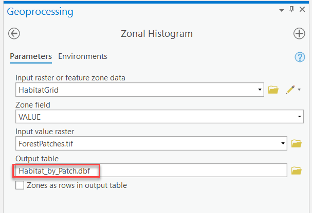
- Open the Zonal Histogram tool (Toolboxes > Spatial Analyst Tools > Zonal > Zonal Histogram). Use the settings below and click "Run." Make sure to add the .dbf extension.
- Open the "Habitat_by_Patch" table. The "LABEL" field contains values equivalent to the "Rowid" field within "ForestPatches." The "VALUE_2" field contains the number of cells of edge habitat for each forest patch. The "VALUE_3" field contains the number of cells of interior habitat for each forest patch (Remember that we used codes of 1, 2, and 3 to represent the different habitat types throughout the lesson).
- These field names are not very intuitive, and we may forget what they mean later on. Let’s add a few new meaningful fields to address this potential problem.
- Add a new short integer field called "ForestID" to the "Habitat_by_Patch" table. Use the calculate field tool to populate it with the values in the “LABEL” field.
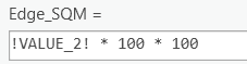
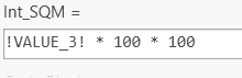
- Add two new float fields named "Edge_SQM" and "Int_SQM." Calculate the fields as shown below (# of cells * cell length * cell width):
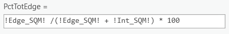
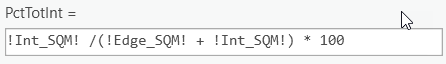
- Remember from Lesson 4 that it is a lot easier to compare multiple area values if you use percent of the total area instead of actual area values. Add two new short integer fields named "PctTotEdge" and "PctTotInt." Calculate the fields as shown below. Notice the 100 in the equation is used to create a percent value and is not related to the 100 value we used in step e, which corresponds to the length and width of the raster cells.
Make sure you have the correct answer before moving on to the next step.
The "Habitat_by_Patch" table should have the following information. If your data does not match this, go back and redo the previous step.
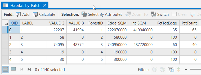 Click here for an accessible alternative to the image above
Accessible Habitat_by_Patch Data Set oid Label Value_2 Value_3 FORESTID EDge_sqm int_sqM PCTtotedge pcttotint 0 1 22207 41994 1 222070000 419940000 35 65 1 2 58 0 2 580000 0 100 0 2 3 74095 48772 3 740950000 487720000 60 40 3 4 19 0 4 190000 0 100 0 4 5 30 0 5 300000 0 100 0
- Open the Zonal Histogram tool (Toolboxes > Spatial Analyst Tools > Zonal > Zonal Histogram). Use the settings below and click "Run." Make sure to add the .dbf extension.
-
Calculate Habitat Statistics by Management Unit
- Use the Zonal Histogram Tool to determine the amount of each habitat type by management unit as shown in the example below: Don’t forget the file extension.
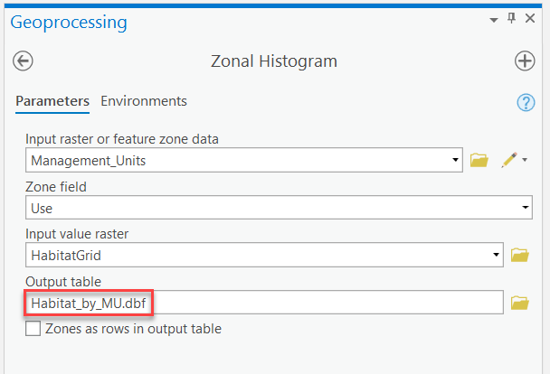
What do numbers in the "LABEL" field of the "Habitat_by_MU" mean? Which management unit "use" has the most roads?
- Add a new text field (length 25) named “Habitat.” Use the field calculator and the information below to update the new field.
- 1 - Low-Quality Habitat (Road Clearings)
- 2 - Medium Quality Habitat (Forest, Edge Habitat)
- 3 - High-Quality Habitat (Forest, Interior Habitat)
- Add two new float fields named “LogSQM” and “ConsSQM.” Add two new short integer fields named “PctTotLog” and “PctTotCons.” Calculate them using the technique we used in Step 2 e and f.
Make sure you have the correct answer before moving on to the next step.
The "Habitat_by_MU" table should have the following values. If your data does not match this, go back and redo the previous step.
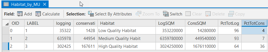 Click here for an accessible alternative to the image above
Accessible Habitat_by_MU dataset OID Label logging coservation habitat logSqm conssqm pcttotlog pcttotcons 0 1 35322 1428 Low Quality Habitat 353220000 14280000 96 4 1 2 635978 44954 Medium Quality Habitat 6359780000 449540000 93 7 2 3 302425 167611 High Quality Habitat 3024250000 1676110000 64 36 -
Join Forest Patches to Geometry Table
- Since we no longer need the forest patches to be in raster format, let’s convert them to a shapefile so they are easier to use.
- Convert the "ForestPatches.tif" grid to a polygon shapefile using the settings below: Toolboxes > Conversion Tools > From Raster > Raster to Polygon.
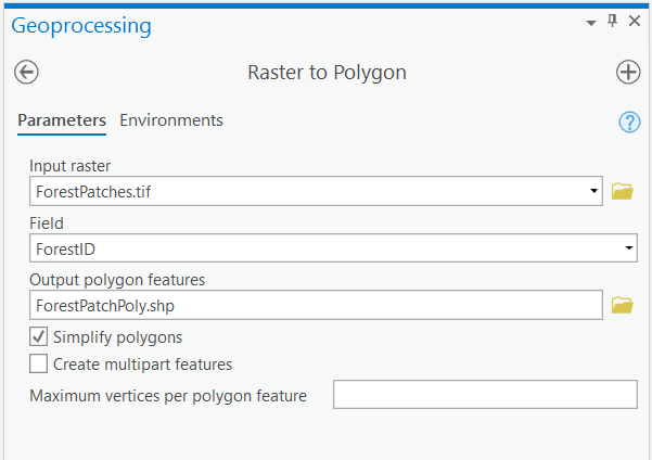
- Add a new short integer field named "FORESTID" and populate it with the values in the "GRIDCODE" field.
Make sure you have the correct answer before moving on to the next step.
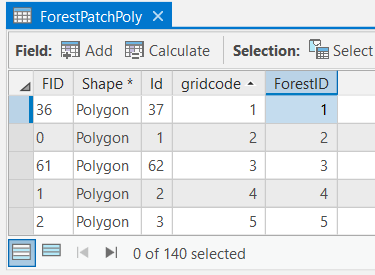
The "forestpatchpoly" shapefile should have the following information. If your data does not match this, go back and redo the previous step. Note that this table has been sorted based on "gridcode".
 Click here for an accessible alternative to the image above
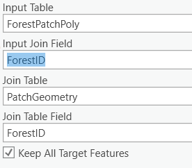
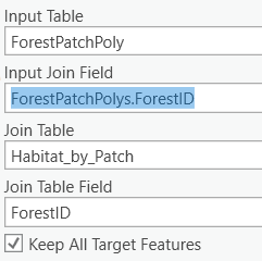
Accessible ForestPatchPoly Data Set Fid Shape* Id gridcode ForestID 36 Polygon 37 1 1 0 Polygon 1 2 2 61 Polygon 62 3 3 1 Polygon 2 4 4 2 Polygon 3 5 5 - Join the "PatchGeometry" and "Habitat_by_Patch" tables to the "forestpatchpoly" shapefile using the link fields shown below.
- Open the attribute table to make sure the joins worked properly. Notice how it is hard to view the attributes we are most interested in since there are so many fields.
- On the ribbon, go to the Table > View tab >Fields
 , and uncheck the "Visible" box on the top left side. Add the checkboxes back to the eight fields listed below and click "Save."
- ForestID
- TotAreaSQM
- PerimeterM
- ThicknessM
- Edge_SQM
- Int_SQM
- PctTotEdge
- PctTotInt
- Close and then re-open the ForestPatchPoly attribute table. Notice how it is much easier to interpret the results now.
- To make the joins and table design permanent, export the "forestpatchpoly" to a new shapefile in your Lesson 7 folder named “Final_Forest_Patches.shp.”
- Examine the attribute table.
-
Calculate the Edge to Area Ratio of each Forest Patch
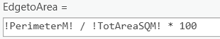
- Calculate the edge to area ratio for each patch. Add a new float field named "EdgetoArea." Calculate it as shown below. Note: we are going to multiply the result by "100" to make the values easier to compare.
Why is there such a large range of values for the edge to area ratio results?
How would the results of the analysis change if we used a larger or smaller cell size?
Make sure you have the correct answer before moving on to the next step.
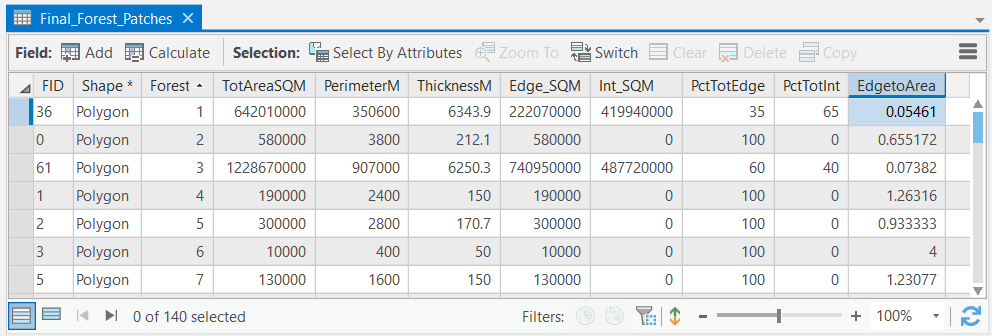
The "Final_Forest_Patches" attribute table should have the following information. If your data does not match this, go back and redo the previous step.
 Click here for an accessible alternative to the image above
Accessible Final_Forest_Patches Dataset FID Shape* Forest ID Totareasqm perimeterm thichnessm edge_sqm int_sqm pcttotedge pcttotint edgetoarea 36 Polygon 1 642010000 350600 6343.9 222070000 419940000 35 65 0.05461 0 Polygon 2 580000 3800 212.1 580000 0 100 0 0.655172 61 Polygon 3 1228670000 90700 6250.3 740950000 487720000 60 40 0.07382 1 Polygon 4 190000 2400 150 190000 0 100 0 1.26316 2 Polygon 5 300000 2800 170.7 300000 0 100 0 0.933333 3 Polygon 6 10000 400 50 10000 0 100 0 4 5 Polygon 7 130000 1600 150 130000 0 100 0 1.23077 Notice how the default outputs from many of the Spatial Analyst tools are not very easy to understand. It’s worth the time to create more intuitive fields, units, and names while you are doing the analysis. That way you can easily interpret your results later on and share them with others in a meaningful format.
- Calculate the edge to area ratio for each patch. Add a new float field named "EdgetoArea." Calculate it as shown below. Note: we are going to multiply the result by "100" to make the values easier to compare.
- Use the Zonal Histogram Tool to determine the amount of each habitat type by management unit as shown in the example below: Don’t forget the file extension.
Part IV: Share Your Results
Part IV: Share Your Results
In Part IV, we will finalize our map in ArcGIS, then you will be asked to share your results with the Geog487 AGO group as web maps. As a final step, you will combine the output from the Step-by-Step and Advanced Activity into a web application.
-
Prepare Your Map to Publish in ArcGIS Online
- When you publish your map to ArcGIS Online, it preserves many of the features such as the extent and visible datasets. Let’s begin by removing all of the data we do not want to include on our final map. Remove the base map, all of the data sets, and all of the tables (you may need to switch to the List by Source view in the Contents pane) from your map except the following: Final_Forest_Patches, Study_Boundary, Roads07, and Management_Units. Save your map.
- Remove the underscores from the file names in the Contents pane.
- Change the symbology of the Final Forest Patches to Quantities > Graduated Colors based on the PctTotEdge field. Select a color scheme and number of classes you think best represent the message you want to convey about the results. You may want to consult ColorBrewer2 [21] for advice and tips.
- Update the labels in the Symbology or Contents pane so the numbers in the Final Forest Patches make sense to your viewers. (What are the units? What’s being shown?)
- Change the symbology of the management units to hollow outlines with a unique color for each “Use.”
- Review your map. Ask yourself the following questions: 1) What are the main messages I am trying to convey with my map? (Remember, you want to show the relationship between logging and forest health.) 2) Does my map design communicate these messages clearly? 3) Will someone unfamiliar with my analysis be able to use my map to make a decision? Make any changes you think are necessary and save your map.
-
Share Your Results with the Group using ArcGIS Online
- If necessary, review Lesson 2 for a refresher on how to share your 2007, 2001 and 2021 Forest Patches maps with our GEOG487, Environmental Applications of GIS Group through the Penn State AGO Enterprise Organization. You can either build a web application or create a story map for the web application requirement listed as Step 2 below.
- Step 1: Publish Three Maps in Penn State's ArcGIS Online for Organizations Account
- Forest Patches 2007 (Final Results from Step-by-Step Activity)
- Forest Patches 2001 (Final Results from Advanced Activity)
- Forest Patches 2021 (Final Results from Advanced Activity)
- Step 2: Create a Web Application in ArcGIS Online that incorporates your Advanced Activity results.
- I encourage you to select a template that allows the reader to easily compare at least two of the maps listed above (e.g., 2007 and 2001 or 2007 and 2021).
That’s it for the required portion of the Lesson 7 Step-by-Step Activity. Please consult the Lesson Checklist for instructions on what to do next.
Try This!
Try one or more of the optional activities listed below.
- Explore the Global Forest Watch Interactive Mapping Website
Many of the data sets we will use in the lesson were originally created by Global Forest Watch [22].
- Explore the USGS Earth Explorer website.
Landsat satellite images were used to digitize the road data we used in this lesson. You can read more about Landsat data on NASA’s website [23]. As of October 2008, Landsat data is available for free to the public. It can be viewed and downloaded from the USGS Earth Explorer Viewer [24].
Note: Try This! Activities are voluntary and are not graded, though I encourage you to complete the activity and share comments about your experience on the lesson discussion board.
Advanced Activity
Advanced Activity
Advanced Activities are designed to make you apply the skills you learned in this lesson to solve an environmental problem and/or explore additional resources related to lesson topics.
Directions:
In the Step-by-Step activity, we used road center-lines from the year 2007 to explore forest fragmentation and edge effects. Using the road centerlines from 2001 (roads01), how many forest patches were located in the study site in 2001? Using the road centerlines from 2021 (roads21), how many forest patches were located in the study site in 2021?
Summary and Deliverables
Summary and Deliverables
In Lesson 7, we used Buffers, the Reclassify Tool, RegionGroup, ZonalGeometry, and Zonal Histograms to explore how logging roads have degraded tropical rainforests in southeastern Cameroon. Specifically, we determined how many forest patches were created, the area and shape of each forest patch, their edge/area ratio, and the area of edge and interior habitat. We also summarized the habitat type by management unit to see whether conservation areas or logging areas provide the best habitat.
Lesson 7 Deliverables
Lesson 7 is worth a total of 100 points.
- Create Web Maps and Application (80 points)
- Step 1: Publish Three Maps in Penn State's ArcGIS Online for Organizations Account
- Forest Patches 2007 (Final Results from Step-by-Step Activity). Include a description.
- Forest Patches 2001 (Final Results from Advanced Activity). Include a description.
- Forest Patches 2021 (Final Results from Advanced Activity). Include a description.
- Step 2: Create a Web Application in ArcGIS Online
- Select a template that allows the reader to easily compare at least two of the maps (e.g., the 2007 and 2021 maps or the 2007 and 2001 maps). Include a description of the app that sufficiently orients the reader and helps to convey trends.
- Map Design Considerations:
- Your web application will be used by the World Bank to make decisions regarding funding in the region. It is important that your map tells a compelling story, or you may lose funding for your team.
- Share the maps and applications you create with the GEOG 487 Group in ArcGIS Online.
- Select colors and break values that are consistent between both maps to make it easier to visually compare the changes over time.
- Include informative and professional map titles, layer names, and legend labels.
- Map descriptions should succinctly summarize the main trends you want your map readers to notice and explain what the map colors mean. What kind of changes do you see between the two years? Why does this matter?
- Include data sources. List other classmates as sources if you consult their work for inspiration.
- Your web application will be used by the World Bank to make decisions regarding funding in the region. It is important that your map tells a compelling story, or you may lose funding for your team.
- Step 3: Share Results
- Post a link to your web application.
- Post a link to your Forest Patches 2007 (Final Results from Step-by-Step Activity).
- Post a link to your Forest Patches 2001 (Final Results from Advanced Activity).
- Post a link to your Forest Patches 2021 (Final Results from Advanced Activity).
- Your maps and app need to be saved in Penn State's ArcGIS Online for Organizations Account and shared with the GEOG487 Group to receive credit.
- Step 1: Publish Three Maps in Penn State's ArcGIS Online for Organizations Account
- Lesson 7 Quiz (20 points)
Peer Review (optional): Explore other students' submission and add a short comment on their discussion post.
| 2007 Forest Patches Map | Web map is posted to ArcGIS Online and link is made available in Canvas. Map is sufficiently designed and described. (20pts) | Map is linked, but it is missing an element or two (layers, descriptions, symbology, etc.) (15pts) | Map is linked but is missing several elements (map, layers, description) or is poorly designed. (10pts) | Link is missing. (0pts) | 20pts |
|---|---|---|---|---|---|
| 2001 Forest Patches Map | Web map is posted to ArcGIS Online and link is made available in Canvas. Map is sufficiently designed and described. (20pts) | Map is linked, but it is missing an element or two (layers, descriptions, symbology, etc.) (15pts) | Map is linked but is missing several elements (map, layers, description) or is poorly designed. (10pts) | Link is missing. (0pts) | 20pts |
| 2021 Forest Patches Map | Web map is posted to ArcGIS Online and link is made available in Canvas. Map is sufficiently designed and described. (20pts) | Map is linked, but it is missing an element or two (layers, descriptions, symbology, etc.) (15pts) | Map is linked but is missing several elements (map, layers, description) or is poorly designed. (10pts) | Link is missing. (0pts) | 20pts |
| Web Map Application | Web app link is posted and made available in Canvas. App facilitates the direct comparison between at least two of the maps (e.g., the 2007 and 2001 maps or the 2007 and 2021 maps). Symbology is consistent between the two maps. Description of the app and maps sufficiently orients the reader and helps to convey trends. (20pts) | Web app link is posted. Some elements of the assignment are missing, but the app still allows for map comparison. (15pts) | Web app link is present but is missing several elements, does not function properly, or otherwise impairs the ability to compare the two maps. (10pts) | Web app link is missing. (0pts) | 20pts |
| TOTAL | 80pts | ||||
Tell us about it!
If you have anything you'd like to comment on, or add to the lesson materials, feel free to post your thoughts in the Lesson 7 Discussion. For example, what did you have the most trouble with in this lesson? Was there anything useful here that you'd like to try in your own workplace?
Additional Resources
Additional Resources
This page includes links to resources such as additional readings and websites related to the lesson concepts. Feel free to explore these on your own. If you'd like to suggest other resources for this list, contact the instructor
Reports:
- Interactive Forestry Atlas [16]
- An Analysis of Access to Central Africa's Rainforests [25]
- The Forests of the Congo Basin - State of the Forest 2008 [26]
- An Overview of Logging in Cameroon [27]
- 9 Maps that Explain the World's Forests [28]
Websites:
- World Resource Institute [29] - Links to WRI's Maps & Data webpages; maps and downloadable GIS data about forests and forest management around the world can be found here.
- Global Forest Watch [30] - Deforestation Alerts
Videos:
- "Working to Save Central Africa's Forests [31]" (3:28)
- Highlights WRI’s work in Central Africa. Contains great images of intact forests, logging practices, and GIS and remote sensing data sets from the region.
- "Independent Forest Monitoring Part 1 [32]" (9:02)
- "Independent Forest Monitoring Part 2 [33]" (9:56)
- A set of videos produced by Global Witness that provide an excellent overview of the logging practices, corruption, and difficulty of monitoring logging activities in Cameroon. They also show how GIS maps and GPS are used to assist in monitoring efforts.
- "Illegal Logging in Cameroon [34]" (4:55)
- Illegal logging is big business in Cameroon. Forty percent of the country is covered by rainforest, but the illicit timber trade places unsustainable pressure on the ecosystem and its communities – which see few benefits from logging.