Lesson 8: Groundwater Vulnerability Modeling
Lesson 8 Overview and Checklist
Lesson 8 Overview
Scenario
You have been hired by the Lake Raystown Watershed Council to identify potential sludge disposal sites within a watershed in south-central Pennsylvania. You must take into account the vulnerability of groundwater contamination, distance from surface water, and area of each potential site. To accomplish this task, you will use ArcGIS Spatial Analyst tools to recode and overlay maps depicting important factors that affect inherent vulnerability. You will then combine your results with information about surface water and site area to identify potential sites for sludge disposal.
Goals
At the successful completion of Lesson 8, you will have:
- calculated slope from Digital Elevation Models;
- created weighted overlays of multiple grids using the Raster Calculator;
- identified suitable locations based on multiple input criteria using Spatial Analyst.
Questions?
- Read all of the pages listed under the Lesson 8 Module.
Read the information on the "Background Information," "Required Readings," "Lesson Data," "Step-by-Step Activity," "Advanced Activities," and "Summary and Deliverables" pages. - Read and watch the required readings and videos.
See the "Required Readings and Videos" page for links. - Download Lesson 8 data.
See the "Lesson Data" page. - Download and complete the Lesson 8 Step-by-Step Activity.
- See the "Step-by-Step Activity" page for a link to a printable PDF of steps to follow.
- Complete the Lesson 8 Advanced Activity.
See the "Advanced Activity" page. - Complete the Lesson 8 Quiz.
See the "Summary and Deliverables" page. - Optional - Check out additional resources.
See the "Additional Resources" page. This section includes links to several types of resources if you are interested in learning more about environmental data covered in this lesson.
If you have questions now or at any point during this lesson, please feel free to post them to the Lesson 8 Discussion.
Background Information
Background Information
Sewage Sludge Disposal
Sewage sludge is the solid waste created during the process of domestic wastewater treatment. This material is often inadvertently contaminated with many toxic organic and inorganic compounds. Lesson 8 focuses on the identification of suitable locations within the Lake Raystown Watershed, where processed sewage sludge can be applied to the soil surface as part of a controlled bio-degradation treatment alternative. There area two primary advantages of this process: 1) the natural renovative capabilities of the soil are used to further break down residuals that remain after standard wastewater treatment processes, and 2) the nutrient-rich sludge material serves as a beneficial soil amendment which can complement, and in many cases replace, standard fertilization practices.
An important consideration in evaluating the suitability of potential sewage disposal sites is the potential impact such sites might have on existing groundwater quality. There are a number of approaches that can be used to evaluate pollution problems associated with groundwater resources, ranging from very complex to relatively simple. An example of a complex approach is the use of sophisticated computer models (such as the MODFLOW model [1] developed by the U.S. Geological Survey) to track the dispersion of contaminants through the soil profile and beyond. While this approach may help one to accurately quantify contaminant movement and loads, it does have a very serious limitation in the form of very extensive data needs. For this reason, simpler, empirical approaches are often used to evaluate pollution potential. One such approach is the DRASTIC methodology developed by the U.S. Environmental Protection Agency.
DRASTIC Methodology
"DRASTIC" is an acronym in which each letter stands for one of seven hydrogeological parameters that directly influence the movement of pollutants into and through the soil and sub-soil layers. Measurements within each parameter are assigned DRASTIC Ratings between 1 and 10 based on how they affect the movement of contaminants. Some of the parameters (e.g., depth to groundwater) have a much greater influence on the overall groundwater vulnerability than others. This is incorporated into the DRASTIC Index calculation by assigning weights to each of the parameters based on their relative importance. Areas with higher DRASTIC Index Scores are more likely to experience groundwater contamination in the event of a release than areas with low DRASTIC Index Scores.
The equation to calculate the DRASTIC Index is:
$$(\mathbf{D} \times 5)+(\mathbf{R} \times 4)+(\mathbf{A} \times 3)+(\mathbf{S} \times 2)+(\mathbf{T} \times 1)+(\mathbf{I} \times 5)+(\mathbf{C} \times 3)$$The seven parameters are briefly described below:
- D - Depth to Groundwater Parameter
- Depth below the surface that groundwater is located.
- DRASTIC Ratings range from 1 (deep depth to groundwater) to 10 (shallow depth to groundwater).
- Relative Importance: highest weight (5).
- R - Net Recharge Parameter
- Rate at which water infiltrates through the soil and into the groundwater.
- DRASTIC Ratings range from 1 (slow recharge rate) to 9 (fast recharge rate).
- Relative Importance: high weight (4).
- A - Aquifer Media Parameter
- Rock type the groundwater (aquifer) is located in.
- DRASTIC Ratings range from 1 (material impedes water movement) to 10 (material encourages groundwater movement).
- Relative Importance: medium weight (3).
- S - Soil Media Parameter
- Soil type the water must travel through to reach the groundwater.
- DRASTIC Ratings range from 1 (material impedes water movement) to 10 (material encourages groundwater movement).
- Relative Importance: low weight (2).
- T - Topography (Slope) Parameter
- How steep or gentle the slope is.
- DRASTIC Ratings range from 1 (steep slope - water likely to run off) to 10 (gentle slope / water likely to infiltrate).
- Relative Importance: lowest weight (1).
- I - Impact of Vadose Zone Parameter
- The vadose zone is the area beneath the surface that is not saturated with groundwater.
- DRASTIC Ratings range from 1 (impedes water movement /breaks down contaminants) to 10 (encourages water movement / does not break down contaminants).
- Relative importance - highest weight (5).
- C - Hydraulic Conductivity Parameter
- Ability of the aquifer to transmit water.
- DRASTIC Ratings range from 1 (low water transmission ability) to 10 (high water transmission ability).
- Relative importance - medium weight (3).
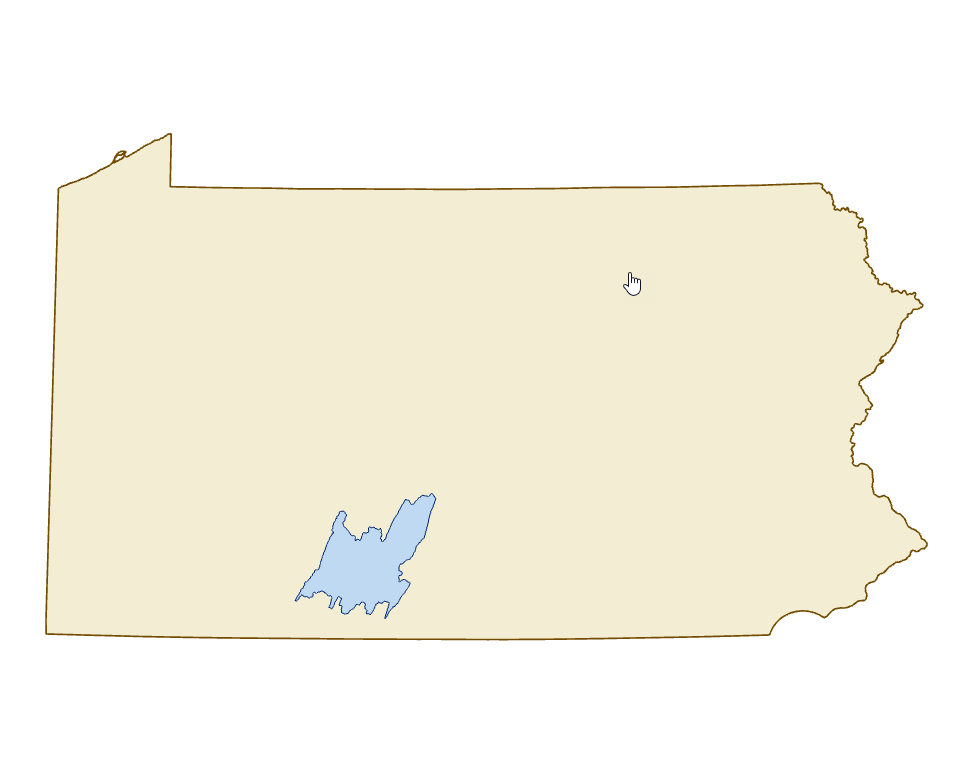
Study Area
The Lake Raystown watershed is located in South Central Pennsylvania and covers an area of approximately 1,000 square miles. Contained within this watershed is Raystown Lake. This man-made recreational lake was created as a flood control dam designed to protect the populated areas from Huntingdon, Pennsylvania to the mouth of the Susquehanna River.
Required Readings
Required Readings
All of the required readings for Lesson 8 are Esri help articles. Although we will demonstrate how to use these tools in the Step-by-Step Activity, the help topics will provide you with a good overview of what the tools will do when executed.
Find the help articles listed below on ArcGIS Pro Resource Center [2] website.
- "How Slope works [3]"
- "What is Map Algebra [4]?"
- "Overview of the Rules for Map Algebra [5]"
- "An Overview of the Map Algebra Operators [6]"
- "Working with Operators in Map Algebra [7]" (pay attention to the "Operator Precedence" section)
- "Extract by Attributes (Spatial Analyst) [8]"
Lesson Data
Lesson Data
This section provides links to download the Lesson 8 data, along with reference information about each dataset (metadata). Briefly review the information below so you have a general idea of the data we will use in this lesson.
For this lesson, you will be provided with all of the data in the Lesson 8 Data zip file. All of these data were created by your own work organization. While receiving data from an in-house source may seem like a blessing, it often comes without some of the typical information you receive from well-known data clearinghouses. Two of the most common shortcomings are a lack of metadata and projection information. Therefore, it may be difficult to determine the source of the data, the attribute definitions, the scale of the data, and the coordinate system and datum. As distressing as this may sound, there will generally be someone in your office who can provide some reliable information pertaining to the data.
Lesson 8 Data Download:
Note: You should not complete this activity until you have read through all of the pages in Lesson 8. See the Lesson 8 Checklist for further information.
Create a new folder in your GEOG487 folder called "L8." Download a zip file of the Lesson 8 Data [9] and save it in your "L8" folder. Extract the zip file and view the contents. Information about all datasets used in the lesson is provided below:
Metadata
Publicly Available Data:
Base Map:
- Source: Esri Resource Center (see Lesson 2 for more details about this site).
- Service Names: OpenStreetMap.
- Within ArcGIS, go to Map tab, Layer group > Basemap.
Private Data (Located Inside the L8 Data Folder):
Spatial Reference Parameters:
- Spatial Reference: NAD_1983_Albers
- Linear Unit: Meter (1.000000)
- Angular Unit: Degree (0.017453292519943295)
- False Easting: 0
- False Northing: 0
- Central Meridian: -78
- Standard Parallel 1: 40
- Standard Parallel 2: 42
- Latitude of Origin: 39
- Datum: D_North_American_1983
Datasets:
- LakeRaystown:
- Data Type: Polygon Shapefile
- Description: Boundary of the Lake Raystown Watershed.
- Elev:
- Data Type: Raster (Grid)
- Description: Elevation in meters.
- Geology:
- Data Type: Polygon Shapefile
- Description: Surface geology (i.e., geologic formations).
- Soil:
- Data Type: Polygon Shapefile
- Description:Generalized soil mapping units.
- Streams_buffer:
- Data Type: Polygon Shapefile
- Description: 300 meter buffer of streams.
- D:
- Data Type: Raster (Grid)
- Description: DRASTIC ratings based on the depth to groundwater (D).
- R:
- Data Type: Raster (Grid)
- Description: DRASTIC ratings based on recharge (R).
- Landgrid:
- Data Type: Raster (Grid)
- Description: Land use classified from satellite imagery.
- 2 = Developed
- 3 = Woodland
- 4 = Water
- 5 = Mined/Disturbed
- 7 = Agriculture
Step-by-Step Activity
Step-by-Step Activity: Overview
Step-by-Step Activity: Overview
The Step-by-Step Activity for Lesson 8 is divided into three parts. In Part I, we will review the relevant datasets and organize your Map. In Part II, we will create a DRASTIC Groundwater Vulnerability grid. In Part III, we will determine suitable land areas for sewage sludge application sites based on the DRASTIC ratings, distance from surface water, and size of each region.
Lesson 8 Step-by-Step Activity Download
Note: You should not complete this step until you have read through all of the pages under the Lesson 8 Module. See the Lesson 8 Checklist for further information.
Part I: Review the Relevant Data Layers and Organize your Map
Part I: Review the Relevant Data Layers and Organize your Map
In Part I, we will review the starting datasets and organize the map for analysis.
-
Unzip the Data for Use in ArcGIS
- Unzip the Lesson 8 data in your L8 folder. Since all of the starting raster format layers are included in this zip file, you do not need to worry about how you unzip the data.
- Familiarize yourself with the contents of the data included with this zip file. Refer to the Lesson Data section for additional information.
-
Organize the Map Document and Familiarize Yourself with the Study Area
Since all of the datasets used in this lesson have the same projection, we do not need to be concerned with the order that we load the data.
- Start ArcGIS, create a new map, and save it in your L8 folder.
- Add the LakeRaystown, geology, soil, elev, and streams_buffer datasets from your L8Data folder. Select No if prompted, "Would you like to create pyramids?"
- Examine the metadata and attribute tables of all of the starting datasets.
- Change the symbology of the "LakeRaystown" and "streams_buffer" layers to hollow outlines, the geology layer to unique values by "rock_type," and the soils layer to unique values by "texture."
- Zoom to the layer extent of the Lake Raystown Watershed and look for spatial patterns in the geology and soil datasets.
- Add the Open Street Map basemap. Explore the study area.

Do the all of the provided raster grids have the same cell size?
Do all of the input datasets have the same extent?
What are the units of the "VALUE" attribute in the elevation grid?
How many different types of soil and rock types are in the study area?
How wide a buffer was used to create the streams data?
Where is the Lake Raystown Watershed located in relation to the state of Pennsylvania?
-
Set the Spatial Analyst Option Settings
- Go to the Analysis tab, Geoprocessing group > Environments
- Set your workspace and scratch space to your Lesson 8 folder.
- Set the output coordinates, mask, and extent to the same as "LakeRaystown.”
- Set the cell size to 30 meters.
- Choose to not build pyramids.
- Save your project to lock in the options.
- Go to the Analysis tab, Geoprocessing group > Environments
Part II: Customize the Data and Produce the DRASTIC Groundwater Vulnerability Layer
Part II: Customize the Data and Produce the DRASTIC Groundwater Vulnerability Layer
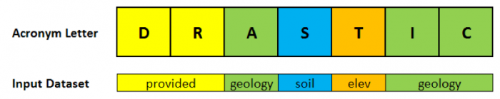
In Part II, we will create a series of grids representing the DRASTIC Ratings for each parameter (D -Depth to Water Table, R- Net Recharge, A - Aquifer Media, S - Soil Media, T - Topography, I - Impact of Vadose Zone, and C- Hydraulic Conductivity). The dataset we will use to create each grid is shown in the graphic below. In this section, we will introduce two new spatial analyst concepts: creating slope grids from elevation and reclassifying ranges of values as opposed to unique values.
-
Add DRASTIC ratings to the Soil Layer
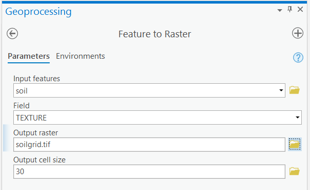
- Open the Soil attribute table and examine the data. Pay particular attention to the "TEXTURE" field. We will use this field to convert the vector file to a raster grid.
- Go to the Analysis tab, Geoprocessing group > Tools > Toolboxes > Conversion Tools > To Raster > Feature to Raster.

Make sure you have the correct answer before moving on to the next step.
The "soilgrid.tif" attribute table should have all of the attributes shown below. If your data does not match this, go back and redo the previous step. Be sure to go to Feature to Raster tool > Environments and double-check and the output coordinates and processing extent to the same as "LakeRaystown.” Also, be sure to expand the table columns to view all COUNT totals.
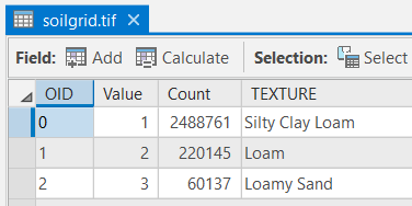
- Compare the "soilgrid.tif" map and attribute table to that of the "soil" shapefile.
- Now that the soil data is in grid format, we can reclassify the grid to assign DRASTIC Ratings to each soil type.
- Use the values in the table below to reclassify "soilgrid.tif" based on the "TEXTURE" field. Name the output file "s.tif" (This is the letter used in the DRASTIC acronym to represent the Soil Media). Be sure to confirm the Reclassify > Environments > output coordinates, processing extent and mask are the same as "LakeRaystown.”
Table 1: DRASTIC Ratings for Soil Textures (S) Texture DRASTIC Rating Silty Clay Loam 3 Loam 5 Loamy Sand 6 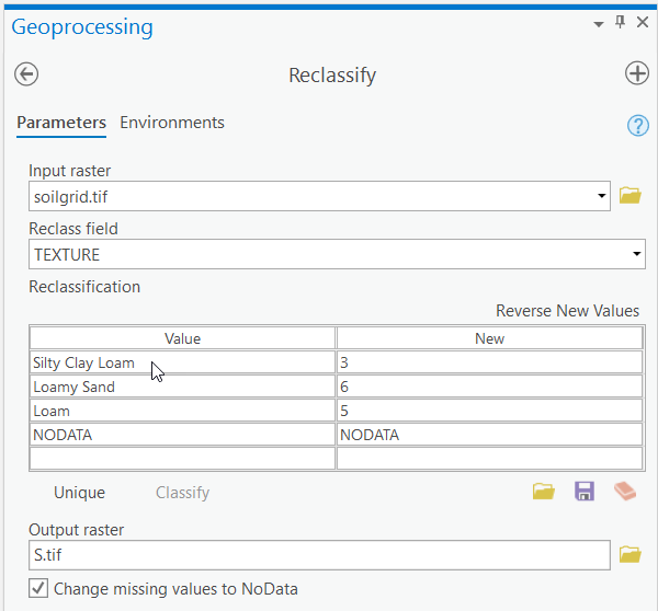
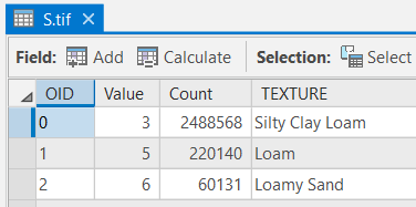
Make sure you have the correct answer before moving on to the next step.
The "s.tif" attribute table should match the example below. If your data does not match this, go back and redo the previous step.
-
Add DRASTIC ratings to the Geology Layer
Three of the seven DRASTIC factors (A - Aquifer media, I - Impact of the vadose zone, and C - Hydraulic Conductivity) can be defined on the basis of geology. We will use the Reclassify Tool again to assign DRASTIC ratings corresponding to these three factors for the appropriate surface geology units contained in the geology layer.
- Open the Geology attribute table and examine the data. Pay particular attention to the "ROCK_TYPE" field. We will use this field to convert the vector file to a raster grid.
- Convert the Geology shapefile to a grid. Use "ROCK_TYPE" as the "Field." Name the grid "geologygrid.tif"
Make sure you have the correct answer before moving on to the next step.
The "geologygrid.tif" attribute table should have all of the attributes shown below. If your data does not match this, go back and redo the previous step.
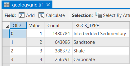 Click here for an accessible text version of the image above
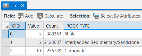
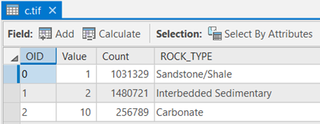
Accessible geologygrid.tif dataset OID Value Count Rock_type 0 1 1480784 Interbedded Sedimentary 1 2 643096 Sandstone 2 3 388372 Shale 3 4 256791 Carbonate - Tables 2, 3, and 4 show the DRASTIC ratings for Aquifer Media, Vadose Zone, and Hydraulic Conductivity, respectively. Create three new grids from the "geology grid" raster .tif using the reclassify tool and "ROCK_TYPE" field. Name the new grids "a.tif," "i.tif," and "c.tif". Remember to confirm the Reclassify > Environments >output coordinates, processing extent and mask are the same as "LakeRaystown.”
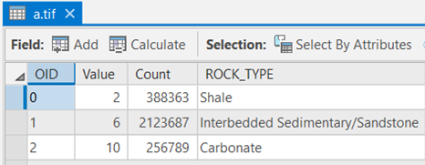
Table 2: DRASTIC Ratings for Aquifer Media (a) Rock Type DRASTIC Rating Interbedded Sedimentary 6 Sandstone 6 Shale 2 Carbonate 10 Table 3: DRASTIC Ratings for Vadose Zone (i) Rock Type DRASTIC Rating Interbedded Sedimentary 6 Sandstone 6 Shale 3 Carbonate 10 Table 4: DRASTIC Ratings for Hydraulic Conductivity (c) Rock Type DRASTIC Rating Interbedded Sedimentary 2 Sandstone 1 Shale 1 Carbonate 10 Make sure you have the correct answer before moving on to the next step.
The "a," "i," and "c" attribute tables should have all of the attributes shown below. If your data does not match this, go back and redo the previous step. Again, be sure to expand the COUNT field to see all the complete values.
-
Create a Slope Map from the Digital Elevation Model and add DRASTIC ratings
When you have data that represents elevation, you can create several different types of raster layers, one is a slope grid. Slope represents steepness, incline, or grade of a line or area. A higher slope value indicates a steeper incline. With Spatial Analyst, it is easy to create a slope layer from elevation data.
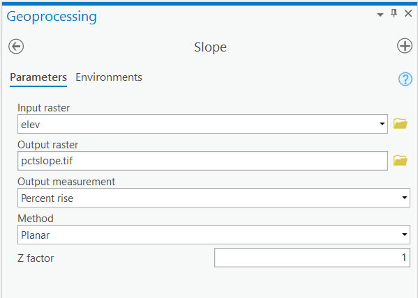
- Go to the Analysis tab, Geoprocessing group > Tools > Toolboxes > Spatial Analyst Tools > Surface > Slope.
- Choose "elev" as the "Input raster", select "PERCENT RISE" for the "Output measurement." Leave the "Z factor" at 1 and name the output raster "pctslope.tif". The resulting layer depicts steep slopes with high values and gentle slopes with low values. Remember to confirm that the Slope > Environments > output coordinates, processing extent, and mask are the same as "LakeRaystown.”

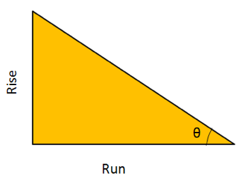
Degree vs. Percentage
Be careful when choosing the slope output measurement. There are two ways to express slope values, either as a percent or as a degree. "45 degrees" slope and "45 %" slope are NOT equivalent values.
Degree slope (θ): angle created by a right triangle with sides of length "rise" and "run"
Percent slope: length of "rise"/length of "run" * 100
- Examine the "pctslope.tif" grid. Notice how the attribute table is greyed out. Remember from Lesson 5 that raster attribute tables are not created if the values contain decimals.
- We want to reclassify the "pctslope.tif" grid using the DRASTIC Ratings in Table 6.
Table 6: Ranges and Ratings for Topography Topography Range DRASTIC Rating 0-2 10 2-6 9 6-12 5 12-18 3 >18 1 - Open the Reclassify tool and select the "pctslope.tif" grid. Notice the default number of classes and break values listed in the "Start" and "End" columns. These are not particularly useful to us, since we want to use 5 break values (2, 6, 12, 18, and the largest number in the dataset).
- The quickest way to change these settings is to click on the "Classify" button. Change the number of classes to "5." Manually type in the break values. "
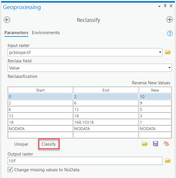
- Modify the "New Values" in the reclassify window based on the values in Table 6. Name the resulting grid "t.tif". Make sure you check the box "Change missing values to NoData" and confirm the Reclassify > Environments > output coordinates, processing extent and mask are the same as "LakeRaystown.”
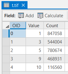
Make sure you have the correct answer before moving on to the next step.
The "t" attribute table should have all of the attributes shown below. If your data does not match this, go back and redo the previous step.
Reclassifying Ranges of Numbers vs. Unique Values
When you need to reclassify data based on ranges of values instead of unique values. For example, notice above that the old value of "2" is specified as the upper bound in the range "0-2" and the lower bound in the range "2-6." What new value, either "10" or "9," will be assigned to old values of "2" in the output grid?
In this case, ArcGIS will assign the old value "2" to a new value of "10," and the old value of "2.0001" to a new value "9" in the output grid. The general rule is that ArcGIS will include the break values themselves in the group that it forms the upper range boundary. Notice that you will encounter this same issue for all break values (e.g., "6", "12", and "18" in the example above).
This is particularly important when the break values themselves are meaningful in your analysis. The most common example of this situation is when you encounter specifications of "less than x" vs. "less than or equal to x" in your requirements. If you want to reclassify values "less than 5" to a new value, you would need to specify a break value of "4.99999999," so the value of "5" is not included in your new category. The particular number of decimals you need to specify will depend on the number of decimals in your input data. For example, if your data layer has five decimal places, then you would set the reclassification thresholds as follows: a.aaaaa - b.bbbbb, b.bbbbb - c.ccccc, and so forth.
See the ArcGIS Help for further information regarding reclassification by range [10].
-
Explore the DRASTIC Rating Output Grids
- Add the "r" and "d" grids from your L8 folder and open the attribute tables. The numbers in the "VALUE" fields correspond with DRASTIC ratings based on each cell’s recharge rate and depth to groundwater, respectively. These are the final input datasets required to calculate DRASTIC groundwater vulnerability ratings for the watershed.
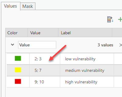
- Change the symbology of the d, r, a, s, t, i, and c grid layers so that low vulnerability ratings (1-3) are green, medium ratings (4-7) are yellow, and high ratings (8-10) are red. You can classify similar values together using "Unique Values" on the Symbology pane > Press the Ctrl key and click to select rows under Value heading to group > Right-click select Group values.
- Update the label column as shown below so the results are easier to interpret.
Compare the "d" grid to the "streams_buffer" shapefile. Do areas near streams have high or low vulnerability?
Which input datasets (d, r, a, s, t, i, c) have the highest DRASTIC rating values?
Do you see any spatial patterns in the individual drastic grids?
- Remove all of the datasets other than the drastic grids, the steam buffers, and the watershed boundary so your map is easier to work with. Save your map.
-
Calculate the DRASTIC Groundwater Vulnerability Index
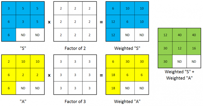
Now that you have the required data layers, you can create a DRASTIC groundwater vulnerability grid based upon the DRASTIC index equation. This will involve use of the Raster Calculator to combine several grids in a weighted overlay. The graphic below shows an example of how cell values are updated during the calculation.
Combining raster layers is a simple, yet very important process with Spatial Analyst. You will often find that it is necessary to create a single layer that is comprised of several data sets. The idea is similar to that of performing an overlay with vector layers, in that you are making one out of many, with the major exception that the cell values change based on the expression used.
The addition (+) and multiplication (*) signs are the most common arithmetic operators used to combine raster layers. The plus (+) sign performs an addition with each cell, so the value in a given cell of one grid will be added to the value of the same cell in the next grid, and so on. The multiplication (*) sign, as expected, performs a multiplication based on the values in each cell.
Either of these can be used when the purpose is to simply combine grids, although you should use the same operator for all grids. However, when forming an expression that includes additional operations on individual grids, as in the case above, it is important to understand the precedence that the operators will be performed. In mathematical order of operation rules, multiplication always takes precedence over addition. Hence, in the expression above, the values in the "D" grid will be multiplied by 5 before they are added to the values in the "R" grid. If an expression should occur that is out of precedence, enclose that expression with parentheses, as you would when using a calculator.
- Open the Raster Calculator Analysis tab, Geoprocessing group > Tools > Toolset > Spatial Analyst Tools > Map Algebra > Raster Calculator) and enter the expression below and name the grid "drastic_index". Be careful when choosing your input files. Also, the syntax for the raster calculator must be absolutely correct, or you will get a "syntax error."
"d" * 5 + "r" * 4 + "a.tif" * 3 + "s.tif" * 2 + "t.tif" * 1 + "i.tif" * 5 + "c.tif" * 3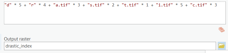
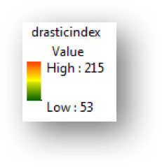
- Change the color ramp so that high values are shades of red and low values are shades of green like the example below.

Make sure you have the correct answer before moving on to the next step.
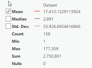
The" drastic_index" grid should have the following information. The statistics from the "COUNT" field are also provided. If your data does not match this, go back and redo the previous step.
What do the numbers in the "VALUE" field of the "drastic_index" mean in the real world? For example, do high values represent areas with high or low vulnerability to groundwater pollution?
Which parts of the watershed are most vulnerable to groundwater pollution?
Do any of the parameters have a greater influence on the final results?
- Open the Raster Calculator Analysis tab, Geoprocessing group > Tools > Toolset > Spatial Analyst Tools > Map Algebra > Raster Calculator) and enter the expression below and name the grid "drastic_index". Be careful when choosing your input files. Also, the syntax for the raster calculator must be absolutely correct, or you will get a "syntax error."
Part III: Identify the Potential Suitable Sites for Sludge Disposal
Part III: Identify the Potential Suitable Sites for Sludge Disposal
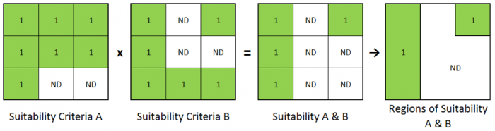
Now that the groundwater vulnerability layer has been produced, we can use this data to help find the areas in the watershed most suitable for sludge disposal. Along with this dataset, we also need to incorporate the stream buffer dataset. Remember from previous lessons that it is possible to reclassify grid cells to values of "NoData" to exclude them from your analysis. We will use this technique to remove portions of each dataset that do not meet the relevant criteria. For example, we will reclassify suitable areas within each dataset as "1" and unsuitable areas as "NoData."
You can also do the opposite of this by assigning existing values of "NoData" to more meaningful values. We will use this technique to create a grid of areas that are outside of steam buffers. Then, we will use the Raster Calculator to combine the individual suitability results into one grid. We will then use the "RegionGroup” command to create regions from adjacent cells with the same results. This process is illustrated in the graphic below.
For the purposes of this lesson, we assume that state regulations require the following for a site to be considered for sludge disposal:
- Areas that are very vulnerable to groundwater contamination must be avoided. Therefore, we will only consider areas with DRASTIC Index values less than 150.
- Sites must be at least 300 meters from surface water.
- Sites must have a contiguous area of at least 0.5 square km.
-
Explore the DRASTIC Rating Output Grids
- In Part II Step 3, we talked about the potential pitfalls of using the reclassify tool when break values are important in your results. One way to avoid this issue is to use the Raster Calculator, which allows us to use mathematical sign of less than or greater than. Enter the expression shown below and name your grid "di150."
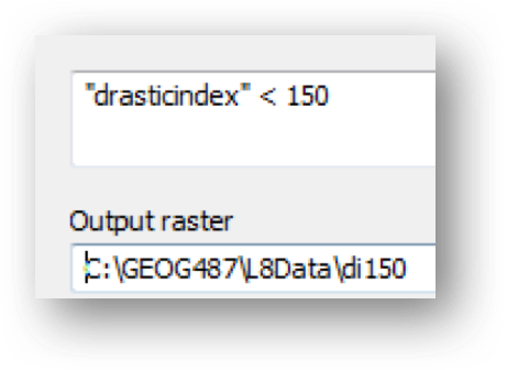
The calculation performed in the previous step combines the results of two Boolean operations that are either evaluated as:
TRUE (indicated by a value of 1) OR FALSE (indicated by a value of 0)
We are only interested in cells that meet the criteria (values of 1).
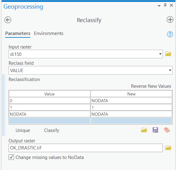
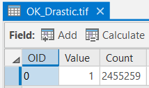
- Reclassify the "di150" grid using the settings below. Name the output grid "OK_Drastic.tif" and confirm the tool Environments.
Make sure you have the correct answer before moving on to the next step.
The "OK_DRASTIC.tif" attribute table should have all of the attributes shown below. If your data does not match this, go back and redo the previous step.
- In Part II Step 3, we talked about the potential pitfalls of using the reclassify tool when break values are important in your results. One way to avoid this issue is to use the Raster Calculator, which allows us to use mathematical sign of less than or greater than. Enter the expression shown below and name your grid "di150."
-
Create a Grid of Suitable Surface Water
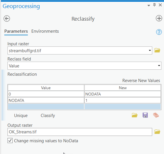
- Convert the "steams_buffer" shapefile to a raster using the "Id" field. Name the output "streambuffgrd.tif" and save it in your L8 folder and confirm the tool Environments.
- Reclassify "streambuffgrd.tif" as shown below. Name the output "OK_Streams.tif" and confirm the tool Environments.
Make sure you have the correct answer before moving on to the next step.
The "OK_Streams" attribute table should have all of the attributes shown below. If your data does not match this, go back and redo the previous step.
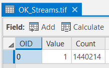
- Compare the "OK_Streams.tif" layer to the "steambuffgrd." Notice how we have essentially flipped the areas of NoData. It is important that you choose an appropriate mask and extent settings when using this technique.
-
Combine the Suitability Grids Using the Raster Calculator
- Use the raster calculator to multiply the "OK_Drastic.tif" and "OK_Streams.tif" rasters together. Cells that meet both of the criteria will be assigned a value of "1" in the output raster. Cells that do not meet either one or both of the criteria will be assigned a value of "NoData" in the output raster. Name the new grid "OK2criteria."
Make sure you have the correct answer before moving on to the next step.
The "OK2criteria.tif" attribute table should have all of the attributes shown below. If your data does not match this, go back and redo the previous step.
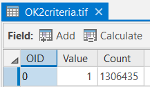
- Examine the attribute table. Notice there is only 1 row. We need a way to lump together cells that make up contiguous units. To accomplish this, we will use the Region Group tool like we did in Lesson 7.
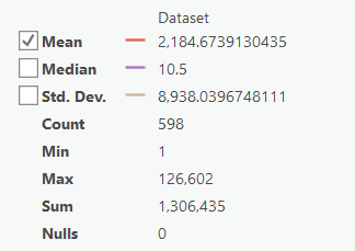
- Go to Toolboxes > Spatial Analyst Tools > Generalization > Region Group, select " OK2criteria.tif" as the input raster, name the output raster " OK_Regions ", leave the number of neighbors to use as "FOUR", the zone grouping method as "WITHIN", uncheck the "Add link field to output", leave the excluded value setting , and click OK.
Make sure you have the correct answer before moving on to the next step.
The "OK_Regions" statistics for the "COUNT" field should match the example below. If your data does not match this, go back and redo the previous step.
- Use the raster calculator to multiply the "OK_Drastic.tif" and "OK_Streams.tif" rasters together. Cells that meet both of the criteria will be assigned a value of "1" in the output raster. Cells that do not meet either one or both of the criteria will be assigned a value of "NoData" in the output raster. Name the new grid "OK2criteria."
-
Create Grid of Suitable Regions Greater than 0.5 sq km
-
The last criteria we need to incorporate is - Area (sites greater than 0.5 sq km). We learned in Lesson 5 that you can calculate the area of a raster by multiplying the number of cells by the area of each cell. To calculate the area of regions within a raster, we can use this same method.
- Add a new float field to the "OK_Regions" attribute table named "AREA_SQM." Use the field calculator to populate the field.
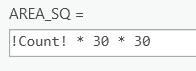
Why did we use the number "30" to calculate the area?
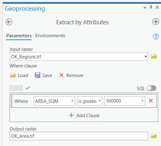
- We will use Extract by Attributes to perform a query on sites > 0.5 sq km. Extract by Attributes is similar to the Raster Calculator, except that it makes entering specific field expressions much easier.
- Go to Toolboxes > Spatial Analyst Tools > Extraction > ExtractByAttributes. Select "OK_Regions.tif" as the input raster and name the output raster "OK_Area". To populate the "Where clause" with the expression given below, click the "Query Builder" button. The "Query Builder" dialog will appear. Click on "AREA_SQM", and then on "greater than or equal to", and type 500000 at the end of the expression (0.5 sq km = 500,000 sq m). Confirm the tool Environments. Click Run to automatically input the expression into the "Where clause."
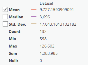
Make sure you have the correct answer before moving on to the next step.
The "OK_Area" statistics for the "COUNT" field should match the example below. If your data does not match this, go back and redo the previous step.
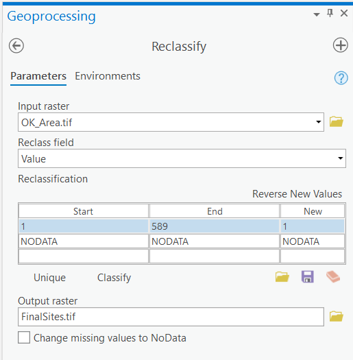
- Reclassify "OK_Area.tif". Change the number of classes to "1," since all of the start and end values match all of the site selection criteria. Name the grid "FinalSites.tif" and confirm the tool Environments. These are your potential sludge disposal sites.
This is all for the required portion of the Lesson 8 Step-by-Step Activity. Please consult the Lesson Checklist for instructions on what to do next.
-
Try This!
Try one or more of the optional activities listed below.
- Redo Part III of the lesson using the value of "0" to denote unsuitable areas instead of "NoData." Compare your results with the "FinalSites.tif" grid.
- Redo Part III of the lesson, except add the suitable grids together instead of multiplying them. How do you need to alter the reclassification values to find suitable sites using this methodology?
Note: Try This! Activities are voluntary and are not graded, though I encourage you to complete the activity and share comments about your experience on the lesson discussion board.
Advanced Activity
Advanced Activity
Advanced Activities are designed to make you apply the skills you learned in this lesson to solve an environmental problem and explore additional resources related to lesson topics.
Directions:
The regulations for sludge disposal sites were revised to help prevent land use change in the watershed. The new regulations require that sludge disposal can only occur on land that is currently used for agriculture. This will prevent areas such as forests and wetlands from being used as disposal sites.
Find suitable sites in the Lake Raystown Watershed that meet all of the following criteria:
- DRASTIC value less than 150;
- at least 300 meters from streams;
- agricultural land use (hint - use the "landgrid" raster layer);
- contiguous area of 0.5 sq km or greater.
Summary and Deliverables
Summary and Deliverables
In Lesson 8, we created a DRASTIC Groundwater Vulnerability grid and identified the potentially suitable sites for sludge disposal. We used Spatial Analyst tools to convert vector into raster data, calculate slope, reclassify grids, and combine multiple rasters. Next week, you will apply the skills and techniques you learned in the course to explore an environmental challenge on your own.
Lesson 8 Deliverables
Lesson 8 is worth a total of 100 points.
- (100 points) Lesson 8 Quiz
Tell us about it!
If you have anything you'd like to comment on, or add to the lesson materials, feel free to post your thoughts in the Lesson 8 Discussion. For example, what did you have the most trouble with in this lesson? Was there anything useful here that you'd like to try in your own workplace?
Additional Resources
Additional Resources
This page includes links to resources such as additional readings and websites related to the lesson concepts. Feel free to explore these on your own. If you'd like to suggest other resources for this list, please send the instructor an email.
Study Site Information:
DRASTIC Information:
- DRASTIC: A Standardized System for Evaluating Ground Water Pollution Potential Using Hydrogeologic Settings [13], Aller et al. (1985)
- Evaluating Ground Water Pollution Potential [14]
- Derivation of a Physiographically-Based Depth to Groundwater Map for the State of Pennsylvania [15], Evans and Anderson (1997)
Sludge Site Screening:
- Sludge Application Site Screening Using a Geographic Information System [16], Brandt et al. (1989)