As we already explained, the idea of a Jupyter Notebook is that it can contain code, the output produced by the code, and rich text that, like in a normal text document, can be styled and include images, tables, equations, etc. Jupyter Notebook is a client-server application meaning that the core Jupyter program can be installed and run locally on your own computer or on a remote server. In both cases, you communicate with it via your web browser to create, edit, and execute your notebooks.
The history of Jupyter Notebook goes back to the year 2001 when Fernando Pérez started the development of IPython, a command shell for Python (and other languages) that provides interactive computing functionalites. In 2007, the IPython team started the development of a notebook system based on IPython for combining text, calculations, and visualizations, and a first version was released in 2011. In 2014, the notebook part was split off from IPython and became Project Jupyter, with IPython being the most common kernel (= program component for running the code in a notebook) for Jupyter but not the only one. There now exist kernels to provide programming language support for Jupyter notebooks for many common languages including Ruby, Perl, Java, C/C++, R, and Matlab.
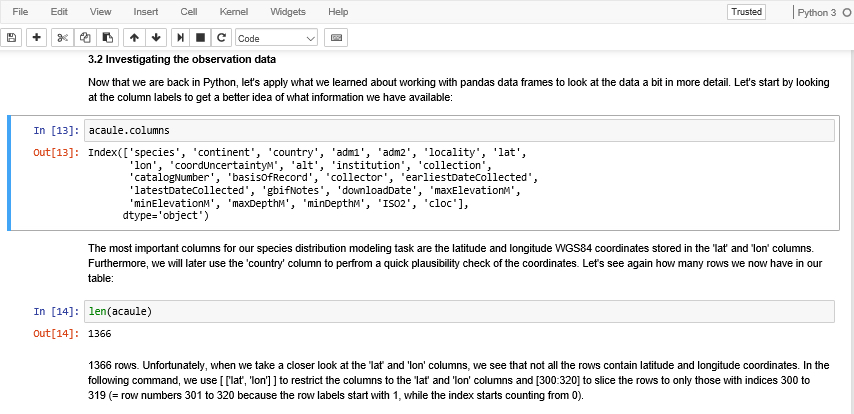
To get a first impression of Jupyter Notebook have a look at Figure 3.2 (which you already saw earlier). The shown excerpt consists of two code cells with Python code (those with starting with “In [...]:“) and the output produced by running the code (“Out[...]:”), and of three different rich text cells before, after, and between the code cells with explanations of what is happening. The currently active cell is marked by the blue bar on the left and frame around it.

Before we continue to discuss what Jupyter Notebook has to offer, let’s get it running on your computer so that you can directly try out the examples.