Before we will start to create another Jupyter notebook with a much more complex example, let us talk about the task and application domain we will be using. As we mentioned at the beginning of the lesson, we will be using a Jupyter notebook to connect Python with R to be able to use some specialized statistical models for the application field of species distribution modeling.
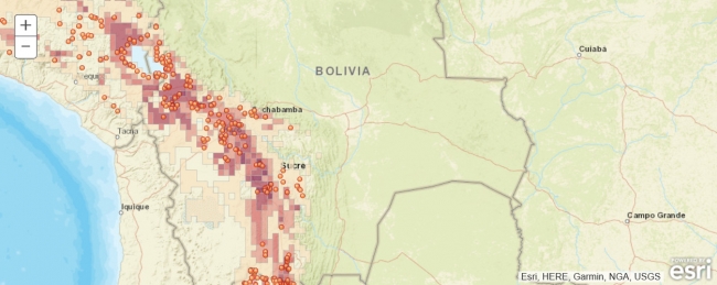
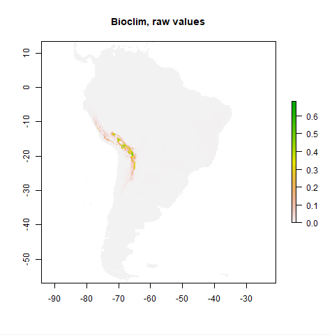
Simply speaking, species distribution modeling is the task or process of predicting the real-world distribution or likelihood of a species occurring at any location on the earth based on (a) existing occurrence and potentially also absence data, e.g. from biological surveys, and (b) data for a number of predictive variables, most often climate related, but also including elevation, soil type, land cover type, etc. The output of a species distribution model is typically a raster with probabilities for the area of interest (which might be the entire earth) that can be used to create a map visualization to help with analysis and decision making. Anticipating the main result of this lesson’s walkthrough, Figure 3.15(b) shows the distribution of Solanum acaule, a plant species growing in the western countries of South America, as predicted by a particular species distribution model that is implemented in the R package ‘dismo’ developed and maintained by Robert J. Hijmans and colleagues. The prediction has been created with the Bioclim model which is one of several models available in dismo.

Teaching you the basics of R is beyond the scope of this course, and you really won’t need R knowledge to follow and understand the short pieces of R code we will be using in this lesson’s walkthrough. However, if you have not worked with R before, you may want to take a quick look through the first five sections of this brief R tutorial (or one of the many other R tutorials on the web). Please note that in this lesson we are not trying to create the best possible distribution model for Solanum acaule (and what actually makes a good or optimal model is something that is heavily debated even among experts anyway). Our main goal is to introduce different Python packages and show how they can be combined to solve spatial analysis tasks inside a Jupyter notebook without letting things get too complex. We, therefore, made quite a few simplifications with regard to what input data to use, how to preprocess it, the species distribution model itself, and how it is applied. As a result, the final model created and shown in the figure above should be taken with a grain of salt.
The ‘dismo’ R package contains a collection of different species modeling approaches as well as many auxiliary functions for obtaining and preprocessing data. See the official documentation of the module. The authors have published detailed additional documentation available in this species distribution modeling document that provides examples and application guidelines for the package and that served as a direct inspiration for this lesson’s walkthrough. One of the main differences is that we will be doing most of the work in Python and only use R and the ‘dismo’ package to obtain some part of the input data and later apply a particular species modeling approach to this data.
Species distribution modeling approaches can roughly be categorized into methods that only use presence data and methods that use both presence and absence data as well as into regression and machine learning based methods. The ‘dismo’ package provides implementations of various models from these different classes but we will only use a rather simple one, the Bioclim model, in this lesson. Bioclim only uses presence data and looks at how close the values of given environmental predictor variables (provided as raster files) for a particular location are to the median values of these variables over the locations where the species has been observed. Because of its simplicity, Bioclim is particularly well suited for teaching purposes.
The creation of a prediction typically consists of the following steps:
- Obtaining and preprocessing of all input data (species presence/absence data and data for environmental predictor variables)
- Creation of the model from the input data
- Using the model to create a prediction based on data for the predictor variables.
require('dismo')
bc <- bioclim(predictorRasters, observationPoints)
You can then use the model to create a Bioclim prediction raster and store it in variable pb and create a plot of the raster with the following R code:
pb <- predict(predictorRasters, bc)
plot(pb, main='Bioclim, raw values')
You may be wondering how you can actually use R commands from inside your Python code. We already mentioned that the magic command %R (or %%R for the cell-oriented version) can be used to invoke R commands within a Python Jupyter notebook. The connection via Python and R is implemented by the rpy2 package that allows for running R inside a Python process. We cannot go into the details of how rpy2 works and how one would use it outside of Jupyter here, so we will just focus on the usage via the %R magic command. To prepare your Jupyter Notebook to interface with R, you will always first have to run the magic command
%load_ext rpy2.ipython
... to load the IPhython rpy2 extension. (If you are trying this out and get an error message about being unable to load the R.dll library, use the following command to manually define the R_HOME environment variable, put in your Windows user ID, and make sure it points to the R folder in your Anaconda AC36/37 environment: os.environ['R_HOME'] = r'C:\Users\youruserid\anaconda3\envs\AC37\lib\R' )
We can then simply execute a single R command by using
%R <command>
To transfer the content of a Python variable to R, we can use
%R –i <name of Python variable>
This creates an R variable with the same name as the Python variable and an R version of the content assigned to it. Similarly,
%R –o <name of R variable>
...can be used for the other direction, so for creating a Python variable with the same name and content as a given R variable. As we will further see in the lesson’s walkthrough, these steps combined make it easy to use R inside a Python Jupyter notebook. However, one additional important component is needed: in R most data used comes in the form of so-called data frames, spreadsheet-like data objects in tabular form in which the content is structured into rows, columns, and cells. R provides a huge collection of operations to read, write, and manipulate data frames. Can we find something similar on the Python side as well that will allow us to work with tabular data (such as attribute information for a set of spatial features) directly in Python? The answer is yes, and the commonly used package to work with tabular data in Python is pandas, so we will talk about it next.