1.5 Working with Python 3 and arcpy in ArcGIS Pro
Now that we’re all warmed up with some Python revision and a few clues about the changes between Python 2 and 3, we’ll start getting familiar with Python 3 in ArcGIS Pro by exploring how we write code and deploy tools just like we did when we started out in GEOG 485.
We’ll cover the conda environment that ArcGIS Pro uses for Python 3 in more detail in Lesson 2, but for now it might be helpful to think of conda as a box or container that Python 3 and all of its parts sit inside. In order to access Python 3, we’ll need to open the conda box, and to do that we will need a command prompt with administrator privileges.
Installing spyder
Spyder is the easiest IDE to install for Python 3 development as we can install it from ArcGIS Pro. Within Pro, you can navigate to the "Project" menu and then choose "Python" to access the Python package and environment manager of the ArcGIS Pro installation.
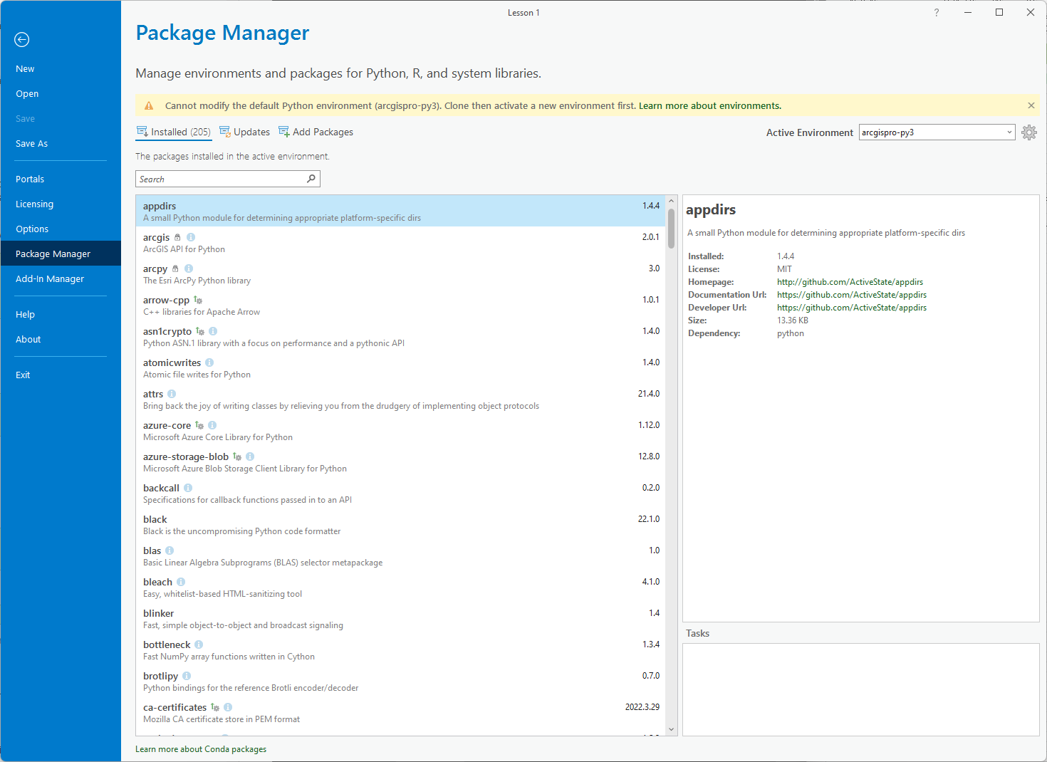
Since version 2.3 of ArcGIS Pro, it is not possible to modify the default Python environment anymore (see here [1] for details). If you already have a working Pro + Spyder setup (e.g. from Geog485) and it is at least Pro version 2.7, you can keep using this installation for this class. Else I'd recommend you work with the newest version, so you will first have to create a clone of Pro's default Python environment and make it the active environment of ArcGIS before installing Spyder. In the past, students sometimes had problems with the cloning operation that we were able to solve by running Pro in admin mode.
Therefore, we recommend that before performing the following steps, you exit Pro and restart it in admin mode by doing a right-click -> Run as administrator. Then go back to "Project" -> "Python", click on "Manage Environments", and then click on "Clone Default" in the Manage Environments dialog that opens up. Installing the clone will take some time (you can watch the individual packages being installed within the "Manage Environments" window and you may be prompted to restart ArcGIS Pro to effect your changes); when it's done, the new environment "arcgispro-py3-clone" (or whatever you choose to call it - but we'll be assuming it's called the default name) can be activated by clicking on the button on the left.
Do so and also note down the path where the cloned environment has been installed appearing below the name. It should be something like C:\Users\<username>\AppData\Local\ESRI\conda\envs\arcgispro-py3-clone . Then click the OK button.
Important: The cloned environment will most likely become unusable when you update Pro to a newer main version (e.g. from 2.9 to 3.0 or 3.0 to 3.1). So once you have cloned the environment successfully, please don't update your Pro installation before the end of the class, unless you are willing to do the cloning and spyder installation again. There is a function in V3.x and later of Pro to update your Python installation but it's new functionality so it might not yet always work as expected.
Now back at the package manager, the new Python environment should appear under "Project Environment" as shown in the figure below (but be aware this might take 30+ minutes so you'll need to be patient).
To now install Spyder, select "Add Packages," search for Spyder and click the "Install" button. This might also take around 30+ minutes and it'll be best if you've restarted Pro after creating your new environment and selecting it.
The package manager will show you a list of packages that will have to be installed and ask you to agree to the terms and conditions. After doing that, the installation will start and probably take a while. You may also get get a "User Access Control" window popup asking if you want conda_uac.exe to make changes to your device; it is OK to choose Yes.
Once the installation is finished, it is recommended that you restart ArcGIS Pro (and if you have trouble restart your PC as well it usually helps). If you keep having problems with the installation failing or Spyder simply not showing up in the list of installed pacakges (even after refereshing the list), please try with starting ArcGIS Pro in admin mode (if you are not already running it this way) by doing a right-click -> Run as administrator.
Once Spyder is installed, you might like to create a shortcut to it on your Desktop or Start Menu. In that case, you should be able to find the Spyder executable in the Scripts subfolder of your cloned Python environment, so at C:\Users\<username>\AppData\Local\ESRI\conda\envs\arcgispro-py3-clone\Scripts\spyder.exe where <username> needs to be replaced with your Windows user name. f you don't see the AppData folder, you will have to change the options in the Windows File Explorer to display hidden files and folders. Make sure to use the .exe file called spyder.exe, not the one called spyder3.exe . If you are using an older version of ArcGIS Pro and installed Spyder directly into the default environment, the path will most likely be C:\Program Files\ArcGIS\Pro\bin\Python\envs\arcgispro-py3\Scripts\spyder.exe .
If you are familiar with another IDE, you're welcome to substitute it for Spyder (just verify that it is using Python 3).
When Spyder launches, it may ask you whether you want to update to a newer version. We recommend to NOT try this because the update procedure will most likely not work with the ArcGIS Pro Python environment. Once Spyder is started, it should display a message in the IPython tab similar to:
Python 3.6.2 |Continuum Analytics, Inc.| (default, Jul 20 2017, 12:30:02) [MSC v.1900 64 bit (AMD64)] Type "copyright", "credits" or "license" for more information. IPython 6.3.1 -- An enhanced Interactive Python.
In [1]:
Don’t worry if the version number is different, as long as it starts with a 3. What we’re looking at here is equivalent to the Python interactive window in ArcGIS Desktop, ArcGIS Pro, PythonWin or any of the IDEs you might be familiar with.
We can experiment here by typing "import arcpy" to import arcpy or running some of those print statement examples from earlier.
In [1]: import arcpy
In [2]: print ("Hello World")
Hello world
You might have noticed while typing in that second example a useful function of the IPython interactive window - code completion. This is where the IDE (spyder does it too) is smart enough to recognize that you're entering a function name and it provides you with the information about the parameters that function takes. If you missed it the first time, enter print( in the IPython window and wait for a second (or less) and the print function's parameters will appear. This also works for arcpy functions (or those from any library that you import). Try it out with arcpy.management.CreateFeatureclass(or your favorite arcpy function).
A first arcpy code example
Click the File menu -> New File option to open a blank code editor window that we can use to write our first piece of Python 3 code with the ArcGIS Pro version of arcpy. In the remainder of this lesson, we’re going to look at some simple examples taken from GEOG 485 (because they should be somewhat familiar to most people) which we’ll use to practice modifying code from Python 2 to 3 where needed and working with arcpy under ArcGIS Pro. Later, we’ll use some of these same code examples to migrate from single processor, sequential execution to multiprocessor, parallel execution. Below, we show the "old" Python 2 version of the code followed by the Python 3 version that you can try out in spyder, e.g. by copying the code into an empty editor window and running it from there.
This first example script reports the spatial reference (coordinate system) of a feature class stored in a geodatabase [2]:
# Opens a feature class from a geodatabase and prints the spatial reference

import arcpy

featureClass = "C:/Data/USA/USA.gdb/States"

# Describe the feature class and get its spatial reference
desc = arcpy.Describe(featureClass)
spatialRef = desc.spatialReference

# Print the spatial reference name
print spatialRef.Name
Python 3 / ArcGIS Pro version:
# Opens a feature class from a geodatabase and prints the spatial reference

import arcpy

featureClass = "C:/Data/USA/USA.gdb/States"

# Describe the feature class and get its spatial reference
desc = arcpy.Describe(featureClass)
spatialRef = desc.spatialReference

# Print the spatial reference name
print (spatialRef.Name)
Did you notice the very subtle difference?
First, let us look at all of the things that are the same and refresh our memories of what the code is doing:
- A comment begins the script to explain what’s going to happen.
- Case sensitivity is applied in the code. "import" is all lower-case. So is "print." The module name "arcpy" is always referred to as "arcpy," not "ARCPY" or "Arcpy." Similarly, "Describe" is capitalized in arcpy.Describe.
- The variable names featureClass, desc, and spatialRef that the programmer assigned are short, but intuitive, and use the camelCase format. By looking at the variable name, you can quickly guess what it represents.
- The script creates objects and uses a combination of properties and methods on those objects to get the job done. That’s how object-oriented programming works.
So, what’s different? The only difference is in the last, highlighted line of the script. The print statement from Python 2 is now a function as we described earlier, so it takes parameters and therefore we’re passing print a value, in this case the spatialRef.Name that we want it to print. That's all!
We’re going to look at a couple more examples (also borrowed from GEOG 485) and convert them from Python 2 to 3 if needed as we continue through the lesson. Esri recognized that a lot of existing Python developers would want to migrate from Python 2 to 3 and to smooth the way they developed a tool for ArcGIS Desktop (which they've since ported to Pro) called Analyze Tools for Pro [3] which does just what the name suggests.
To test the example code we just investigated manually, we saved the Python 2 version to a .py file and supplied it as input to the tool. The output we get from this displaying all of the elements which need to be converted as warnings is shown below.
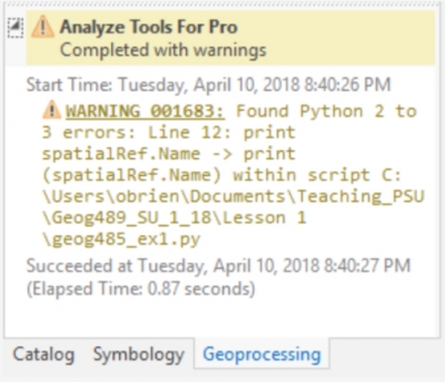
As you can see from the image, we get a warning about the print statement (on line 12) as well as a suggestion of what to change that line to. Those warnings are also written into our output file which will be helpful when we’re trying to modify longer pieces of code (or if you wanted to share the task among many programmers).
1.5.1 Making a Script Tool
Here’s another simple script that finds all cells over 3500 meters in an elevation raster and makes a new raster that codes all those cells as 1. Remaining values in the new raster are coded as 0. By now, you’re probably familiar with this type of “map algebra” operation which is common in site selection and other GIS scenarios.
Just in case you’ve forgotten, the expression Raster(inRaster) tells arcpy that it needs to treat your inRaster variable as a raster dataset so that you can perform map algebra on it. If you didn't do this, the script would treat inRaster as just a literal string of characters (the path) instead of a raster dataset.
# This script uses map algebra to find values in an
#  elevation raster greater than 3500 (meters).

import arcpy
from arcpy.sa import *

# Specify the input raster
inRaster = "C:/Data/Elevation/foxlake"
cutoffElevation = 3500

# Check out the Spatial Analyst extension
arcpy.CheckOutExtension("Spatial")

# Make a map algebra expression and save the resulting raster
outRaster = Raster(inRaster) > cutoffElevation
outRaster.save("C:/Data/Elevation/foxlake_hi_10")

# Check in the Spatial Analyst extension now that you're done
arcpy.CheckInExtension("Spatial")
You can probably easily work out what this script is doing but, just in case, the main points to remember on this script are:
- Notice the lines of code that check out the Spatial Analyst extension before doing any map algebra and check it back in after finishing. Because each line of code takes some time to run, avoid putting unnecessary code between checkout and checkin. This allows others in your organization to use the extension if licenses are limited. The extension automatically gets checked back in when your script ends, thus some of the Esri code examples you will see do not check it in. However, it is a good practice to explicitly check it in, just in case you have some long code that needs to execute afterward, or in case your script crashes and against your intentions "hangs onto" the license.
- inRaster begins as a string, but is then used to create a Raster object once you run Raster(inRaster). A Raster object is a special object used for working with raster datasets in ArcGIS. It's not available in just any Python script: you can use it only if you import the arcpy module at the top of your script.
- cutoffElevation is a number variable that you declare early in your script and then use later on when you build the map algebra expression for your outRaster.
- The expression outRaster = Raster(inRaster) > cutoffElevation is saying, in plain terms, "Make a new raster and call it outRaster. Do this by taking all the cells of the raster dataset at the path of inRaster that are greater than the number assigned to the variable cutoffElevation."
- outRaster is also a Raster object, but you have to call the method outRaster.save() in order to make it permanent on disk. The save() method takes one argument, which is the path to which you want to save.
Copy the code above into a file called Lesson1A.py (or similar as long as it has a .py extension) in spyder or your favorite IDE or text editor and then save it.
We don’t need to do anything to this code to get it to work in Python 3, it will be fine just as it is. Feel free to check it against Analyze Tools for Pro if you like. Your results should say “Analyze Tools for Pro Completed Successfully” with the lack of warnings signifying that the code you supplied is compatible with Python 3.
Next, we'll convert the script to a Tool.
1.5.1.1 Converting the script to a tool
Now, let’s convert this script to a script tool in ArcGIS Pro to familiarize ourselves with the process and we’ll examine the differences between ArcGIS Desktop and ArcGIS Pro when it comes to working with script tools (hint: there aren’t any other than the interface looking slightly different).
We’ll get started by opening ArcGIS Pro. You will be prompted to sign in (use your Penn State ArcGIS Online account which you should already have) and create a project when Pro starts.
Signing in to ArcGIS Pro is an important, new development for running code in Pro as compared to Desktop. As you may be aware, Pro operates with a different licensing structure such that it will regularly "phone home" to Esri's license servers to check that you have a valid license. With Desktop, once you had installed it and set up your license, you could run it for the 12 months the license was valid, online or offline, without any issues. As Pro will regularly check-in with Esri, we need to be mindful that if our code stops working due to an extension not being licensed error or due to a more generic licensing issue, we should check that Pro is still signed in. For nearly everyone, this won't be an issue as you'll generally be using Pro on an Internet connected computer and you won't notice the licensing checks. If you take your computer offline for an extended period, you will need to investigate Esri's offline licensing options [4].
Projects are Pro’s way of keeping all of your maps, layouts, tasks, data, toolboxes etc. organized. If you’re coming from Desktop, think of it as an MXD with a few more features (such as allowing multiple layouts for your maps).
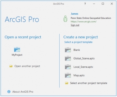
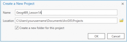
Choose to Create a new project using the Blank template, give it a meaningful name and put it in a folder appropriate for your local machine (things will look slightly different in version 3.0 of Pro: simply click on the Map option under New Project there if you are using that version).
You will then have Pro running with your own toolbox already created. In the figure below, I’ve clicked on the Toolboxes to expand it to show the toolbox which has the same name as my project.
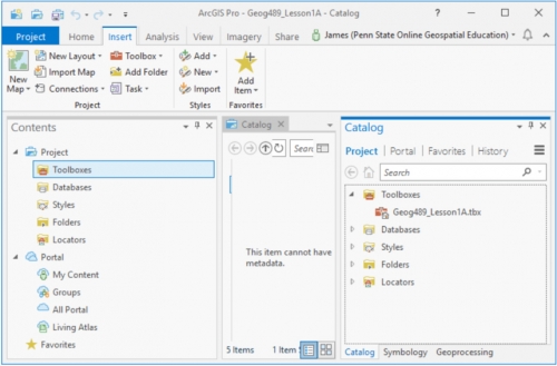
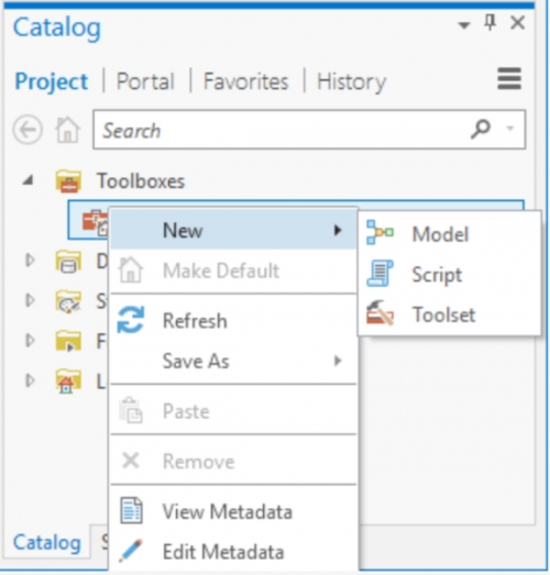
If we right-click on our toolbox we can choose to create a New > Script.
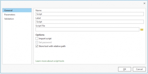
A window will pop up allowing us to enter a name for our script (“Lesson1A”) and a label for our script (“Geog 489 Lesson 1A”), and then we’ll use the file browse icon to locate the script file we saved earlier. In new versions of Pro (2.9 and 3.0), the script file now has to be selected in a new tab called "Execution" located below "Parameters". If your script isn’t showing up in that folder or you get a message that says “Container is empty” press F5 on your keyboard to refresh the view.
We won’t choose to “Import Script” or define any parameters (yet) or investigate validation (yet). When we click OK, we’ll have our script tool created in Pro. We’re not going to run our script tool (yet) as it’s currently expecting to find the foxlake DEM data in C:\data\elevation and write the results back to that folder which is not very convenient. It also has the hardcoded cutoff of 3500 embedded in the code. You can download the FoxLake DEM here [5].
To make the script more user-friendly, we’re going to make a few changes to allow us to pick the location of the input and output files as well as allow the user to input the cutoff value. Later we’ll also use validation to check whether that cutoff value falls inside the range of values present in the raster and, if not, we’ll change it.
We can edit our script from within Pro, but if we do that it opens in Notepad which isn’t the best environment for coding. You can use Notepad if you like, but I’d suggest opening the script again in your favorite text editor (I like Notepad++) or just using spyder.
If you want, you can change this preferred editor by modifying Pro’s geoprocessing options (see http://pro.arcgis.com/en/pro-app/help/analysis/geoprocessing/basics/geoprocessing-options.htm). To access these options in Pro, click Home -> Options -> Geoprocessing Options. Here you can also choose an option to automatically validate tools and scripts for Pro compatibility (so you don’t need to run the Analyze Tools for Pro manually each time).
We're going to make a few changes to our code now, swapping out the hardcoded paths in lines 8 and 17 and the hardcoded cutoffElevation value in line 9. We’re also setting up an outPath variable in line 10 and setting it to arcpy.env.workspace.
You might recall from GEOG 485 or your other experience with Desktop that the default workspace in Desktop is usually default.gdb in your user path. Pro is smarter than that and sets the default workspace to be the geodatabase of your project. We’ll take advantage of that to put our output raster into our project workspace. Note the difference in the type of parameter we’re using in lines 8 & 9. It’s ok for us to get the path as Text, but we don’t want to get the number in cutoffElevation as Text because we need it to be a number.
To simplify the programming, we’ll specify a different parameter type in Pro and let that be passed through to our script. To make that happen, we’ll use GetParameter instead of GetParameterAsText.
# This script uses map algebra to find values in an
#  elevation raster greater than 3500 (meters).

import arcpy
from arcpy.sa import *

# Specify the input raster
inRaster = arcpy.GetParameterAsText(0)
cutoffElevation = arcpy.GetParameter(1)
outPath = arcpy.env.workspace

# Check out the Spatial Analyst extension
arcpy.CheckOutExtension("Spatial")

# Make a map algebra expression and save the resulting raster
outRaster = Raster(inRaster) > cutoffElevation
outRaster.save(outPath+"/foxlake_hi_10")

# Check in the Spatial Analyst extension now that you're done
arcpy.CheckInExtension("Spatial")
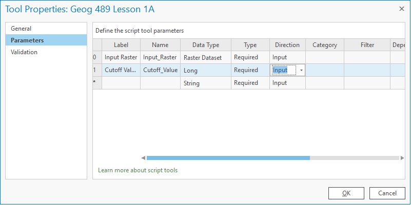
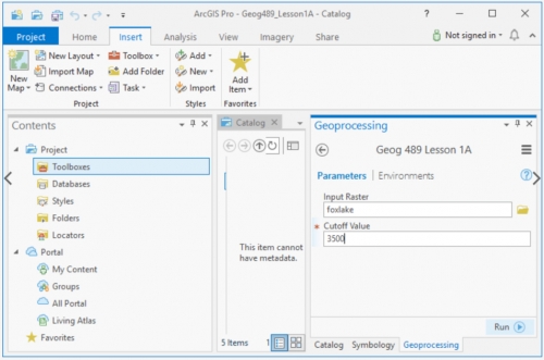
Once you have made those changes, save the file and we’ll go back to our script tool in Pro and update it to use the parameters we’ve just defined. Right click on the script tool within the toolbox and choose Properties and then click Parameters. The first parameter we defined (remember Python counts from 0) was the path to our input raster (inRaster), so let's set that up. Click in the text box under Label and type “Input Raster” and when you click into Name you’ll see that Name is already automatically populated for you. Next, click the Data Type (currently String) and change it to “Raster Dataset” and we’ll leave the other values with their defaults.
Click the next Label text box below your first parameter (currently numbered with a *) and type “Cutoff Value” and change the Data Type to Long (which is a type of number) and we’ll keep the rest of the defaults here too. The final version should look as in the figure below.
Click OK and then we’ll run the tool to test the changes we made by double-clicking it. Use the file icon alongside our Input Raster parameter to navigate to your foxlake raster (which is the FoxLake digital elevation model (DEM) in your Lesson 1 data folder) and then enter 3500 into the cutoff value parameter and click OK to run the tool.
The tool should have executed without errors and placed a raster called foxlake_hi_10 into your project geodatabase.
If it doesn’t work the first time, verify that:
- you have supplied the correct input and output paths;
- your path name contains forward slashes (/) or double backslashes (\\), not single backslashes (\);
- the Spatial Analyst Extension is available. To check this, go Project -> Licensing and check under Esri Extensions;
- you do not have any of the datasets open in ArcGIS;
- the output data does not exist yet. If you want to be able to overwrite the output, you need to add the line "arcpy.env.overwriteOutput = True." This line can be placed immediately after " import arcpy."
1.5.1.2 Adding tool validation code
Now let’s expand on the user friendliness of the tool by using the validator methods to ensure that our cutoff value falls within the minimum and maximum values of our raster (otherwise performing the analysis is a waste of resources).
The purpose of the validation process is to allow us to have some customizable behavior depending on what values we have in our tool parameters. For example, we might want to make sure a value is within a range as in this case (although we could do that within our code as well), or we might want to offer a user different options if they provide a point feature class instead of a polygon feature class, or different options if they select a different type of field (e.g. a string vs. a numeric type).
The Esri help for Tool Validation [6] gives a longer list of uses and also explains the difference between internal validation (what Desktop & Pro do for us already) and the validation that we are going to do here which works in concert with that internal validation.
You will notice in the help that Esri specifically tells us not to do what I’m doing in this example – running geoprocessing tools. The reason for this is they generally take a long time to run. In this case, however, we’re using a very simple tool which gets the minimum & maximum raster values and therefore executes very quickly. We wouldn’t want to run an intersection or a buffer operation for example in the ToolValidator, but for something very small and fast such as this value checking, I would argue that it’s ok to break Esri’s rule. You will probably also note that Esri hints that it’s ok to do this by using Describe to get the properties of a feature class and we’re not really doing anything different except we’re getting the properties of a raster.
So how do we do it? Go back to your tool (either in the Toolbox for your Project, Results, or the Recent Tools section of the Geoprocessing sidebar), right click and choose Properties and then Validation.
You will notice that we have a pre-written, Esri-provided class definition here. We will talk about how class definitions look in Python in Lesson 4 but the comments in this code should give you an idea of what the different parts are for. We’ll populate this template with the lines of code that we need. For now, it is sufficient to understand that different methods (initializeParameters(), updateParameters(), etc.) are defined that will be called by the script tool dialog to perform the operations described in the documentation strings following each line starting with def.
Take the code below and use it to overwrite what is in your ToolValidator:
import arcpy

class ToolValidator(object):
    """Class for validating a tool's parameter values and controlling
    the behavior of the tool's dialog."""

    def __init__(self):
        """Setup arcpy and the list of tool parameters."""
        self.params = arcpy.GetParameterInfo()

    def initializeParameters(self):
        """Refine the properties of a tool's parameters. This method is
        called when the tool is opened."""

    def updateParameters(self):
        """Modify the values and properties of parameters before internal
        validation is performed. This method is called whenever a parameter
        has been changed."""

    def updateMessages(self):
        """Modify the messages created by internal validation for each tool
        parameter. This method is called after internal validation."""
        ## Remove any existing messages
        self.params[1].clearMessage()

        if self.params[1].value is not None:
            ## Get the raster path/name from the first [0] parameter as text
            inRaster1 = self.params[0].valueAsText
            ## calculate the minimum value of the raster and store in a variable
            elevMINResult = arcpy.GetRasterProperties_management(inRaster1, "MINIMUM")
            ## calculate the maximum value of the raster and store in a variable
            elevMAXResult = arcpy.GetRasterProperties_management(inRaster1, "MAXIMUM")
            ## convert those values to floating points
            elevMin = float(elevMINResult.getOutput(0))
            elevMax = float(elevMAXResult.getOutput(0))

            ## calculate a new cutoff value if the original wasn't suitable but only if the user hasn't specified a value.
            if self.params[1].value < elevMin or self.params[1].value > elevMax:
                cutoffValue = elevMin + ((elevMax-elevMin)/100*90)
                self.params[1].value = cutoffValue
                self.params[1].setWarningMessage("Cutoff Value was outside the range of ["+str(elevMin)+","+str(elevMax)+"] supplied raster so a 90% value was calculated")
Our logic here is to take the raster supplied by the user and determine the min and max values so that we can evaluate whether the cutoff value supplied by the user falls within that range. If that is not the case, we're going to do a simple mathematical calculation to find the value 90% of the way between the min and max values and suggest that as a default to the user (by putting it into the parameter). We’ll also display a warning message to the user telling them that the value has been adjusted and why their original value doesn’t work.
As you look over the code, you’ll see that all of the work is being done in the bottom function updateMessages(). This function is called after the updateParameters() and the internal arcpy validation code have been executed. It is mainly intended for modifying the warning or error messages produced by the internal validation code. The reason why we are putting all our validation code here is because we want to produce the warning message and there is no entirely simple way to do this if we already perform the validation and potentially automatic adjustment of the cutoff value in updateParameters() instead. Here is what happens in the updateMessages() function:
We start by cleaning up any previous messages self.params[1].clearMessages() (line 24). Then we check if the user has entered a value into the cutoffValue parameter (self.params[1]) on line 26. If they haven't, we don’t do anything (for efficiency). If the user has entered a value (i.e., the value is not None) then we get the raster name from the first parameter (self.params[0]) and we extract it as text (because we want the content to use as a path) on line 28. Then we’ll call the arcpy GetRasterProperties function twice, once to get the min value (line 30) and again to get the max value (on line 32) of the raster. We’ll then convert those values to floating point numbers (lines 34 & 35).
Once we’ve done that, we do a little bit of checking to see if the value the user supplied is within the range of the raster. If it is not, then we will do some simple math to calculate a value that falls 90% of the way into the range and then update the parameter (self.params[1].value) with the number we calculated (line 40 and 41). Finally, in line 42, we produce the warning message informing the users of the automatic value adjustment.
Now let’s test our Validator. Click OK and return to your script in the Toolbox, Results or Geoprocessing window. Run the script again. Insert the name of the input raster again. If you didn’t make any mistakes entering the code there won’t be a red X by the Input Raster. If you did make a mistake, an error message will be displayed there, showing you the usual arcpy / geoprocessing error message and the line of code that the error is occurring on. If you have to do any debugging, exit the script, return to the Toolbox, right click the script and go back to the Tool Validator and correct the error. Repeat as many times as necessary.
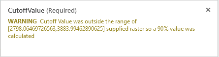
If there were no errors, we should test out our validation by putting a value into our Cutoff Value parameter that we know to be outside the range of our data. If you choose a value < 2798 or > 3884, you should see a yellow warning triangle appear that displays our error message, and you will also note that the value in Cutoff Value has been updated to our 90% value.
We can change the value to one we know works within the range (e.g. 3500), and now the tool should run.