Lesson 3 Python Geo and Data Science Packages & Jupyter Notebooks
3.1 Overview and Checklist
This lesson is two weeks in length. We will introduce a few more Python programming concepts and then focus on conducting (spatial) data science projects in Python with the help of Jupyter Notebooks. In the process, you will get to know quite a few more useful Python packages and 3rd-party APIs including pandas, GDAL/OGR, and the Esri ArcGIS for Python API.
Please refer to the Calendar for specific time frames and due dates. To finish this lesson, you must complete the activities listed below. You may find it useful to print this page first so that you can follow along with the directions.
| Step | Activity | Access/Directions |
|---|---|---|
| 1 | Engage with Lesson 3 Content | Begin with 3.2 Installing the required packages for this lesson |
| 3 |
Programming Assignment and Reflection |
Submit your code for the programming assignment and 400 words write-up with reflections |
| 4 | Quiz 3 | Complete the Lesson 3 Quiz |
| 5 | Questions/Comments | Remember to visit the Lesson 2 Discussion Forum to post/answer any questions or comments pertaining to Lesson 3 |
3.2 Installing the required packages for this lesson
This lesson will require quite a few different Python packages. We will take care of this task right away so that you then won't have to stop for installations when working through the lesson content. We will use our Anaconda installation from Lesson 2 and create a fresh Python environment within it. In principle, you could perform all the installations with a number of conda installation commands from the command line. However, there are a lot of dependencies between the packages and it is relatively easy to run into some conflicts that are difficult to resolve. Therefore, we instead provide a YAML .yml file that lists all the packages we want in the environment with the exact version and build numbers we need. We create the new environment by importing this .yml file using conda in the command line interface ("Anaconda Prompt"). For reference, we also provide the conda commands used to create this environment at the end of this section. Also important to note is that one of the packages we will be working with in this lesson is the ESRI ArcGIS for Python API, which will require a special approach to authenticate with your PSU login. You will already see this approach further down below and it will then be explained further in Section 3.10.
Creating the Anaconda Python environment
Please follow the steps below and if you get issues we've got an alternative approach below.
If you're having issues you'll notice adjacent links to download a YAML file and to use that everywhere below you see "37" please replace it with "38" even if you've got v3.9 - there's no current technical difference between v3.8 & v3.9 for this lesson and in reality the ac37 should work no matter which version you're using. That might sound a little confusing but you should be ok with the AC37 file but just in case we've got some fallbacks. If you have trouble creating the environment from the YAML file there's specific instructions below.
1) Download the .zip file containing the .yml file from this link: ac37_Fall2023.zip [1] (AC38_SP24.zip [2] only if required), then extract the file .yml it contains. You may want to have a quick look at the content of this text file to see how, among other things, it lists the names of all packages for this environment with version and build numbers. Using a YAML file greatly speeds up the creation of the environment as the files are downloaded and dependencies don't need to be resolved on the fly by conda.
2) Open the program called "Anaconda Prompt" which is part of the Anaconda installation from Lesson 2.
3) Make sure you have at least 5GB space on your C: drive (the environment will require around 3.5-4GB). Then type in and run the following conda command to create a new environment called AC37 (for Anaconda Python 3.7 or AC38 for Python 3.8) from the downloaded .yml file. You will have to replace the ... to match the name of the .yml file and maybe also adapt the path to the .yml file depending on where you have it stored on your harddisk.
conda env create --name AC37 -f "C:\489\ac37_....yml"
Conda will now create the environment called AC37 (AC38 if you're using that other file above for Python v3.8) according to the package list in the YAML file. This can take quite a lot of time; in particular, it will just say "Solving environment" for quite a while before anything starts to happen. If you want, you can work through the next few sections of the lesson while the installation is running. The first section that will require this new Python environment is Section 3.6. Everything before that can still be done in the ArcGIS environment you used for the first two lessons. When the installation is done, the AC37 (AC38 for Python v3.8) environment will show up in the environments list in the Anaconda Navigator and will be located at C:\Users\<user name>\Anaconda3\envs\AC37 .
4) Let's now do a quick test to see if the new environment works as intended. In the Anaconda Prompt, activate the new environment with the following command (you'll need to activate your environment every time you want to use it):
activate AC37
Then type in python and in Python run the following commands; all the modules should import without any error messages:
import bs4
import pandas
import cartopy
import matplotlib
from osgeo import gdal
import geopandas
import rpy2
import shapely
import arcgis
from arcgis.gis import GIS
As a last step, let's test connecting to ArcGIS Online with the ArcGIS for Python API mentioned at the beginning. Run the following Python command:
gis = GIS('https://pennstate.maps.arcgis.com', client_id='lDSJ3yfux2gkFBYc')
Now a browser window should open up where you have to authenticate with your PSU login credentials (unless you are already logged in to Penn State). After authenticating successfully, you will get a window saying "OAuth2 Approval" and a box with a very long code at the bottom. In the Anaconda Prompt window, you will see a prompt saying "Enter code obtained on signing in using SAML:". Use CTRL+A and CTRL+C to copy the entire code, and then do a right-click with the mouse to paste the code into the Anaconda Prompt window. The code won't show up, so just continue by pressing Enter.
If you are having troubles with this step, Figure 3.18 in Section 3.10 illustrates the steps. You may get a short warning message (InsecureRequestWarning) but as long as you don't get a long error message, everything should be fine. You can test this by running this final command:
print(gis.users.me)
This should produce an output string that includes your pennstate ArcGIS Online user name, so e.g., <User username:xyz12_pennstate> . More details on this way of connecting with ArcGIS Online will be provided in Section 3.10.
If creating the environment from the .yml file did NOT work:
Creating the AC37 environment from scratch with Conda
As we wrote above, importing the .yml file with the complete package and version number list is probably the most reliable method to set up the Python environment for this lesson but there have been cases in the past where using this approach failed on some systems. Or maybe you are interested in the steps that were taken to create the environment from scratch. We therefore list the conda commands used from the Anaconda Prompt for reference below.
1) Create a new conda Python 3.7 environment called AC37 with some of the most critical packages:
conda create -n AC37 -c conda-forge -c esri python=3.7 nodejs arcgis=2 gdal=3 jupyter ipywidgets=7.6.0
2) As we did in Lesson 2, we activate the new environment using:
activate AC37
3) Then we add the remaining packages:
conda install -c conda-forge rpy2=3.4.1
conda install -c conda-forge r-raster=3.4_5
conda install -c conda-forge r-dismo=1.3_3
conda install -c conda-forge r-maptools
conda install -c conda-forge geopandas
conda install -c conda-forge cartopy
4) Once we have made sure that everything is working correctly in this new environment, we can export a YAML file similar to the one we have been using in the first part above using the command:
conda env export > AC37.yml
If creating the environment from the AC38.yml file did NOT work:
Creating the AC38 environment from scratch with Conda
As we wrote above, importing the .yml file with the complete package and version number list is probably the most reliable method to set up the Python environment for this lesson but there have been cases in the past where using this approach failed on some systems. Or maybe you are interested in the steps that were taken to create the environment from scratch. We therefore list the conda commands used from the Anaconda Prompt for reference below.
1) Create a new conda Python 3.8 environment called AC38 with some of the most critical packages (and you'll notice there's some additional package version numbers specified to handle inconsistencies in V3.8/V3.9):
conda create -n AC38 -c conda-forge -c esri python=3.8 nodejs arcgis=2 gdal=3 jupyter ipywidgets=7.6.0 requests=2.29.0 urllib3=1.26.18
2) As we did in Lesson 2, we activate the new environment using:
activate AC38
3) Then we add the remaining packages:
conda install -c conda-forge rpy2=3.4.1
conda install -c conda-forge r-raster=3.4_5
conda install -c conda-forge r-dismo=1.3_3
conda install -c conda-forge r-maptools
conda install -c conda-forge geopandas
conda install -c conda-forge cartopy  matplotlib=3.5.3 pillow=9.2.0 shapely=1.8.5 fiona=1.8.22
4) Once we have made sure that everything is working correctly in this new environment, we can export a YAML file similar to the one we have been using in the first part above using the command:
conda env export > AC38.yml
Potential issues
There is a small chance that the from osgeo import gdal will throw an error about DLLs not being found on the path which looks like the below:
During handling of the above exception, another exception occurred:
Traceback (most recent call last):

	  File "<stdin>", line 1, in <module>

	  File "C:\Users\jao160\anaconda3\envs\AC38_SP24\lib\site-packages\osgeo\__init__.py", line 46, in <module>

	    _gdal = swig_import_helper()

	  File "C:\Users\jao160\anaconda3\envs\AC38_SP24\lib\site-packages\osgeo\__init__.py", line 42, in swig_import_helper

	    raise ImportError(traceback_string + '\n' + msg)

	ImportError: Traceback (most recent call last):

	  File "C:\Users\jao160\anaconda3\envs\AC38_SP24\lib\site-packages\osgeo\__init__.py", line 30, in swig_import_helper

	    return importlib.import_module(mname)

	  File "C:\Users\jao160\anaconda3\envs\AC38_SP24\lib\importlib\__init__.py", line 127, in import_module

	    return _bootstrap._gcd_import(name[level:], package, level)

	  File "<frozen importlib._bootstrap>", line 1014, in _gcd_import

	  File "<frozen importlib._bootstrap>", line 991, in _find_and_load

	  File "<frozen importlib._bootstrap>", line 975, in _find_and_load_unlocked

	  File "<frozen importlib._bootstrap>", line 657, in _load_unlocked

	  File "<frozen importlib._bootstrap>", line 556, in module_from_spec

	  File "<frozen importlib._bootstrap_external>", line 1166, in create_module

	  File "<frozen importlib._bootstrap>", line 219, in _call_with_frames_removed

	ImportError: DLL load failed while importing _gdal: The specified module could not be found.
On Windows, with Python >= 3.8, DLLs are no longer imported from the PATH.

	If gdalXXX.dll is in the PATH, then set the USE_PATH_FOR_GDAL_PYTHON=YES environment variable

	to feed the PATH into os.add_dll_directory().
In the event this happens the fix is to (every time you want to import gdal you would need to do this):
import os

	os.environ["USE_PATH_FOR_GDAL_PYTHON"]="YES"

	from osgeo import gdal
It's possible the above fix doesn't work and the error is still thrown which will require checking the PATH environment variable in the Anaconda Prompt by typing "path" and checking that c:\osgeo42\bin or osgeo4w64\bin is in the list and if not adding it using set path=%PATH%;c:\osgeo4w\bin
3.3 Regular expressions
To start off Lesson 3, we want to talk about a situation that you regularly encounter in programming: Often you need to find a string or all strings that match a particular pattern among a given set of strings.
For instance, you may have a list of names of persons and need all names from that list whose last name starts with the letter ‘J’. Or, you want do something with all files in a folder whose names contain the sequence of numbers “154” and that have the file extension “.shp”. Or, you want to find all occurrences where the word “red” is followed by the word “green” with at most two words in between in a longer text.
Support for these kinds of matching tasks is available in most programming languages based on an approach for denoting string patterns that is called regular expressions.
A regular expression is a string in which certain characters like '.', '*', '(', ')', etc. and certain combinations of characters are given special meanings to represent other characters and sequences of other characters. Surely you have already seen the expression “*.txt” to stand for all files with arbitrary names but ending in “.txt”.
To give you another example before we approach this topic more systematically, the following regular expression “a.*b” in Python stands for all strings that start with the character ‘a’ followed by an arbitrary sequence of characters, followed by a ‘b’. The dot here represents all characters and the star stands for an arbitrary number of repetitions. Therefore, this pattern would, for instance, match the strings 'acb', 'acdb', 'acdbb', etc.
Regular expressions like these can be used in functions provided by the programming language that, for instance, compare the expression to another string and then determine whether that string matches the pattern from the regular expression or not. Using such a function and applying it to, for example, a list of person names or file names allows us to perform some task only with those items from the list that match the given pattern.
In Python, the package from the standard library that provides support for regular expressions together with the functions for working with regular expressions is simply called “re”. The function for comparing a regular expression to another string and telling us whether the string matches the expression is called match(...). Let’s create a small example to learn how to write regular expressions. In this example, we have a list of names in a variable called personList, and we loop through this list comparing each name to a regular expression given in variable pattern and print out the name if it matches the pattern.
import re

personList = [ 'Julia Smith', 'Francis Drake', 'Michael Mason',
                'Jennifer Johnson', 'John Williams', 'Susanne Walker',
                'Kermit the Frog', 'Dr. Melissa Franklin', 'Papa John',
                'Walter John Miller', 'Frank Michael Robertson', 'Richard Robertson',
                'Erik D. White', 'Vincent van Gogh', 'Dr. Dr. Matthew Malone',
                'Rebecca Clark' ]

pattern = "John"

for person in personList:
    if re.match(pattern, person):
        print(person)
Output:

John Williams
Before we try out different regular expressions with the code above, we want to mention that the part of the code following the name list is better written in the following way:
pattern = "John"

compiledRE = re.compile(pattern)

for person in personList:
    if compiledRE.match(person):
        print(person)
Whenever we call a function from the “re” module like match(…) and provide the regular expression as a parameter to that function, the function will do some preprocessing of the regular expression and compile it into some data structure that allows for matching strings to that pattern efficiently. If we want to match several strings to the same pattern, as we are doing with the for-loop here, it is more time efficient to explicitly perform this preprocessing and store the compiled pattern in a variable, and then invoke the match(…) method of that compiled pattern. In addition, explicitly compiling the pattern allows for providing additional parameters, e.g. when you want the matching to be done in a case-insensitive manner. In the code above, compiling the pattern happens in line 3 with the call of the re.compile(…) function and the compiled pattern is stored in variable compiledRE. Instead of the match(…) function, we now invoke the method match(…) of the compiled pattern object in variable person (line 6) that only needs one parameter, the string that should be matched to the pattern. Using this approach, the compilation of the pattern only happens once instead of once for each name from the list as in the first version.
One important thing to know about match(…) is that it always tries to match the pattern to the beginning of the given string but it allows for the string to contain additional characters after the entire pattern has been matched. That is the reason why when running the code above, the simple regular expression “John” matches “John Williams” but neither “Jennifer Johnson”, “Papa John”, nor “Walter John Miller”. You may wonder how you would then ever write a pattern that only matches strings that end in a certain sequence of characters. The answer is that Python's regular expressions use the special characters ^ and $ to represent the beginning or the end of a string and this allows us to deal with such situations as we will see a bit further below.
Now let’s have a look at the different special characters and some examples using them in combination with the name list code from above. Here is a brief overview of the characters and their purpose:
| Character | Purpose |
|---|---|
| . | stands for a single arbitrary character |
| [ ] | are used to define classes of characters and match any character of that class |
| ( ) | are used to define groups consisting of multiple characters in a sequence |
| + | stands for arbitrarily many repetitions of the previous character or group but at least one occurrence |
| * | stands for arbitrarily many repetitions of the previous character or group including no occurrence |
| ? | stands for zero or one occurrence of the previous character or group, so basically says that the character or group is optional |
| {m,n} | stands for at least m and at most n repetitions of the previous group where m and n are integer numbers |
| ^ | stands for the beginning of the string |
| $ | stands for the end of the string |
| | | stands between two characters or groups and matches either only the left or only the right character/group, so it is used to define alternatives |
| \ | is used in combination with the next character to define special classes of characters |
Since the dot stands for any character, the regular expression “.u” can be used to get all names that have the letter ‘u’ as the second character. Give this a try by using “.u” for the regular expression in line 1 of the code from the previous example.
pattern = ".u"
The output will be:
Julia Smith
Susanne Walker
Similarly, we can use “..cha” to get all names that start with two arbitrary characters followed by the character sequence resulting in “Michael Mason” and “Richard Robertson” being the only matches. By the way, it is strongly recommended that you experiment a bit in this section by modifying the patterns used in the examples. If in some case you don’t understand the results you are getting, feel free to post this as a question on the course forums.
Maybe you are wondering how one would use the different special characters in the verbatim sense, e.g. to find all names that contain a dot. This is done by putting a backslash in front of them, so \. for the dot, \? for the question mark, and so on. If you want to match a single backslash in a regular expression, this needs to be represented by a double backslash in the regular expression. However, one has to be careful here when writing this regular expression as a string literal in the Python code because of the string escaping mechanism, a sequence of two backslashes will only produce a single backslash in the string character sequence. Therefore, you actually have to use four backslashes, "xyz\\\\xyz" to produce the correct regular expression involving a single backslash. Or you use a raw string in which escaping is disabled, so r"xyz\\xyz". Here is one example that uses \. to search for names with a dot as the third character returning “Dr. Melissa Franklin” and “Dr. Dr. Matthew Malone” as the only results:
pattern = "..\."
Next, let us combine the dot (.) with the star (*) symbol that stands for the repetition of the previous character. The pattern “.*John” can be used to find all names that contain the character sequence “John”. The .* at the beginning can match any sequence of characters of arbitrary length from the . class (so any available character). For Instance, for the name “Jennifer Johnson”, the .* matches the sequence “Jennifer “ produced from nine characters from the . class and since this is followed by the character sequence “John”, the entire name matches the regular expression.
pattern = ".*John"
Output:

Jennifer Johnson
John Williams
Papa John
Walter John Miller
Please note that the name “John Williams” is a valid match because the * also includes zero occurrences of the preceding character, so “.*John” will also match “John” at the beginning of a string.
The dot used in the previous examples is a special character for representing an entire class of characters, namely any character. It is also possible to define your own class of characters within a regular expression with the help of the squared brackets. For instance, [abco] stands for the class consisting of only the characters ‘a’, ‘b’,‘c’ and ‘o’. When it is used in a regular expression, it matches any of these four characters. So the pattern “.[abco]” can, for instance, be used to get all names that have either ‘a’, ‘b’, ‘c’ or ‘o’ as the second character. This means using ...
pattern = ".[abco]"
... we get the output:
John Williams
Papa John
Walter John Miller
When defining classes, we can make use of ranges of characters denoted by a hyphen. For instance, the range m-o stands for the lower-case characters ‘m’, ‘n’, ‘o’ . The class [m-oM-O.] would then consist of the characters ‘m’, ‘n’, ‘o’, ‘M’, ‘N’, ‘O’, and ‘.’ . Please note that when a special character appears within the squared brackets of a class definition (like the dot in this example), it is used in its verbatim sense. Try out this idea of using ranges with the following example:
pattern = "......[m-oM-O.]"
The output will be...
Papa John
Frank Michael Robertson
Erik D. White
Dr. Dr. Matthew Malone
… because these are the only names that have a character from the class [m-oM-O.] as the seventh character.
In addition to the dot, there are more predefined classes of characters available in Python for cases that commonly appear in regular expressions. For instance, these can be used to match any digit or any non-digit. Predefined classes are denoted by a backslash followed by a particular character, like \d for a single decimal digit, so the characters 0 to 9. The following table lists the most important predefined classes:
| Predefined class | Description |
|---|---|
| \d | stands for any decimal digit 0…9 |
| \D | stands for any character that is not a digit |
| \s | stands for any whitespace character (whitespace characters include the space, tab, and newline character) |
| \S | stands for any non-whitespace character |
| \w | stands for any alphanumeric character (alphanumeric characters are all Latin letters a-z and A-Z, Arabic digits 0…9, and the underscore character) |
| \W | stands for any non-alphanumeric character |
To give one example, the following pattern can be used to get all names in which “John” appears not as a single word but as part of a longer name (either first or last name). This means it is followed by at least one character that is not a whitespace which is represented by the \S in the regular expression used. The only name that matches this pattern is “Jennifer Johnson”.
pattern = ".*John\S"
In addition to the *, there are more special characters for denoting certain cases of repetitions of a character or a group. + stands for arbitrarily many occurrences but, in contrast to *, the character or group needs to occur at least once. ? stands for zero or one occurrence of the character or group. That means it is used when a character or sequence of characters is optional in a pattern. Finally, the most general form {m,n} says that the previous character or group needs to occur at least m times and at most n times.
If we use “.+John” instead of “.*John” in an earlier example, we will only get the names that contain “John” but preceded by one or more other characters.
pattern = ".+John"
Output:

Jennifer Johnson
Papa John
Walter John Miller
By writing ...
pattern = ".{11,11}[A-Z]"
... we get all names that have an upper-case character as the 12th character. The result will be “Kermit the Frog”. This is a bit easier and less error-prone than writing “………..[A-Z]”.
Lastly, the pattern “.*li?a” can be used to get all names that contain the character sequences ‘la’ or ‘lia’.
pattern = ".*li?a"
Output:

Julia Smith
John Williams
Rebecca Clark
So far we have only used the different repetition matching operators *, +, {m,n}, and ? for occurrences of a single specific character. When used after a class, these operators stand for a certain number of occurrences of characters from that class. For instance, the following pattern can be used to search for names that contain a word that only consists of lower-case letters (a-z) like “Kermit the Frog” and “Vincent van Gogh”. We use \s to represent the required whitespaces before and after the word and then [a-z]+ for an arbitrarily long sequence of lower-case letters but consisting of at least one letter.
pattern = ".*\s[a-z]+\s"
Sequences of characters can be grouped together with the help of parentheses (…) and then be followed by a repetition operator to represent a certain number of occurrences of that sequence of characters. For instance, the following pattern can be used to get all names where the first name starts with the letter ‘M’ taking into account that names may have a ‘Dr. ’ as prefix. In the pattern, we use the group (Dr.\s) followed by the ? operator to say that the name can start with that group but doesn’t have to. Then we have the upper-case M followed by .*\s to make sure there is a white space character later in the string so that we can be reasonably sure this is the first name.
pattern = "(Dr.\s)?M.*\s"
Output:

Michael Mason
Dr. Melissa Franklin
You may have noticed that there is a person with two doctor titles in the list whose first name also starts with an ‘M’ and that it is currently not captured by the pattern because the ? operator will match at most one occurrence of the group. By changing the ? to a * , we can match an arbitrary number of doctor titles.
pattern = "(Dr.\s)*M.*\s"
Output:

Michael Mason
Dr. Melissa Franklin
Dr. Dr. Matthew Malone
Similarly to how we have the if-else statement to realize case distinctions in addition to loop based repetitions in normal Python, regular expression can make use of the | character to define alternatives. For instance, (nn|ss) can be used to get all names that contain either the sequence “nn” or the sequence “ss” (or both):
pattern = ".*(nn|ss)"
Output:

Jennifer Johnson
Susanne Walker
Dr. Melissa Franklin
As we already mentioned, ^ and $ represent the beginning and end of a string, respectively. Let’s say we want to get all names from the list that end in “John”. This can be done using the following regular expression:
pattern = ".*John$"
Output:

Papa John
Here is a more complicated example. We want all names that contain “John” as a single word independent of whether “John” appears at the beginning, somewhere in the middle, or at the end of the name. However, we want to exclude cases in which “John” appears as part of longer word (like “Johnson”). A first idea could be to use ".*\sJohn\s" to achieve this making sure that there are whitespace characters before and after “John”. However, this will match neither “John Williams” nor “Papa John” because the beginning and end of the string are not whitespace characters. What we can do is use the pattern "(^|.*\s)John" to say that John needs to be preceded either by the beginning of the string or an arbitrary sequence of characters followed by a whitespace. Similarly, "John(\s|$)" requires that John be succeeded either by a whitespace or by the end of the string. Taken together we get the following regular expressions:
pattern = "(^|.*\s)John(\s|$)"
Output:

John Williams
Papa John
Walter John Miller
An alternative would be to use the regular expression "(.*\s)?John(\s.*)?$" That uses the optional operator ? rather than | . There are often several ways to express the same thing in a regular expression. Also, as you start to see here, the different special matching operators can be combined and nested to form arbitrarily complex regular expressions. You will practice writing regular expressions like this a bit more in the practice exercises and in the homework assignment.
In addition to the main special characters we explained in this section, there are certain extension operators available denoted as (?x...) where the x can be one of several special characters determining the meaning of the operator. We here just briefly want to mention the operator (?!...) for negative lookahead assertion because we will use it later in the lesson's walkthrough to filter files in a folder. Negative lookahead extension means that what comes before the (?!...) can only be matched if it isn't followed by the expression given for the ... . For instance, if we want to find all names that contain John but not followed by "son" as in "Johnson", we could use the following expression:
pattern = ".*John(?!son)"
Output:

John Williams
Papa John
Walter John Miller
If match(…) does not find a match, it will return the special value None. That’s why we can use it with an if-statement as we have been doing in all the previous examples. However, if a match is found it will not simply return True but a match object that can be used to get further information, for instance about which part of the string matched the pattern. The match object provides the methods group() for getting the matched part as a string, start() for getting the character index of the starting position of the match, end() for getting the character index of the end position of the match, and span() to get both start and end indices as a tuple. The example below shows how one would use the returned matching object to get further information and the output produced by its four methods for the pattern “John” matching the string “John Williams”:
pattern = "John"
compiledRE = re.compile(pattern)

for person in personList:
     match = compiledRE.match(person)
     if match:
         print(match.group())
         print(match.start())
         print(match.end())
         print(match.span())
Output:

John      <- output of group()
0         <- output of start()
4         <- output of end()
(0,4)     <- output of span()
In addition to match(…), there are three more matching functions defined in the re module. Like match(…), these all exist as standalone functions taking a regular expression and a string as parameters, and as methods to be invoked for a compiled pattern. Here is a brief overview:
- search(…) - In contrast to match(…), search(…) tries to find matching locations anywhere within the string not just matches starting at the beginning. That means “^John” used with search(…) corresponds to “John” used with match(…), and “.*John” used with match(…) corresponds to “John” used with search(…). However, “corresponds” here only means that a match will be found in exactly the same cases but the output by the different methods of the returned matching object will still vary.
- findall(…) - In contrast to match(…) and search(…), findall(…) will identify all substrings in the given string that match the regular expression and return these matches as a list.
- finditer(…) – finditer(…) works like findall(…) but returns the matches found not as a list but as a so-called iterator object.
By now you should have enough understanding of regular expressions to cover maybe ~80 to 90% of the cases that you encounter in typical programming. However, there are quite a few additional aspects and details that we did not cover here that you potentially need when dealing with rather sophisticated cases of regular-expression-based matching. The full documentation of the “re” package can be found here [5] and is always a good source for looking up details when needed. In addition, this HOWTO [6] provides a good overview.
We also want to mention that regular expressions are very common in programming and matching with them is very efficient, but they do have certain limitations in their expressivity. For instance, it is impossible to write a regular expression for names with the first and last name starting with the same character. Or, you cannot define a regular pattern for all strings that are palindromes, so words that read the same forward and backward. For these kinds of patterns, certain extensions to the concept of a regular expression are needed. One generalization of regular expressions are what are called recursive regular expressions. The regex [7] Python package currently under development, backward compatible to re, and planned to replace re at some point, has this capability, so feel free to check it out if you are interested in this topic.
3.4 Higher order functions
Higher order functions and lambda expressions
In this section, we are going to introduce a new and very powerful concept of Python (and other programming languages), namely the idea that functions can be given as parameters to other functions similar to how we have been doing so far with other types of values like numbers, strings, or lists. Actually, you have already seen examples of this, namely in Lesson 1 with the pool.starmap(...) function and in Lesson 2 when passing the name of a function to the connect(...) method when connecting a signal to an event handler function. A function that takes other functions as arguments is often called a higher order function.
Let us immediately start with an example: Let’s say you often need to apply certain string functions to each string in a list of strings. Sometimes you want to convert the strings from the list to be all in upper-case characters, sometimes to be all in lower-case characters, sometimes you need to turn them into all lower-case characters but have the first character capitalized, or apply some completely different conversion. The following example shows how one can write a single function for all these cases and then pass the function to apply to each list element as a parameter to this new function:
def applyToEachString(stringFunction, stringList):
	myList = []
	for item in stringList:
		myList.append(stringFunction(item))
	return myList

allUpperCase = applyToEachString(str.upper, ['Building', 'ROAD', 'tree'] )
print(allUpperCase)
As you can see, the function definition specifies two parameters; the first one is for passing a function that takes a string and returns either a new string from it or some other value. The second parameter is for passing along a list of strings. In line 7, we call our function with using str.upper for the first parameter and a list with three words for the second parameter. The word list intentionally uses different forms of capitalization. upper() is a string method that turns the string it is called for into all upper-case characters. Since this a method and not a function, we have to use the name of the class (str) as a prefix, so “str.upper”. It is important that there are no parentheses () after upper because that would mean that the function will be called immediately and only its return value would be passed to applyToEachString(…).
In the function body, we simply create an empty list in variable myList, go through the elements of the list that is passed in parameter stringList, and then in line 4 call the function that is passed in parameter stringFunction to an element from the list. The result is appended to list myList and, at the end of the function, we return that list with the modified strings. The output you will get is the following:
['BUILDING', 'ROAD', 'TREE']
If we now want to use the same function to turn everything into all lower-case characters, we just have to pass the name of the lower() function instead, like this:
allLowerCase = applyToEachString(str.lower, ['Building', 'ROAD', 'tree'] )
print(allLowerCase)
Output:

['building', 'road', 'tree']
You may at this point say that this is more complicated than using a simple list comprehension that does the same, like:
[ s.upper() for s in ['Building', 'ROAD', 'tree'] ]
That is true in this case but we are just creating some simple examples that are easy to understand here. For now, trust us that there are more complicated cases of higher-order functions that cannot be formulated via list comprehension.
For converting all strings into strings that only have the first character capitalized, we first write our own function that does this for a single string. There actually is a string method called capitalize() that could be used for this, but let’s pretend it doesn’t exist to show how to use applyToEachString(…) with a self-defined function.
def capitalizeFirstCharacter(s):
	return s[:1].upper() + s[1:].lower()

allCapitalized = applyToEachString(capitalizeFirstCharacter, ['Building', 'ROAD', 'tree'] )
print(allCapitalized)
Output:

['Building', 'Road', 'Tree']
The code for capitalizeFirstCharacter(…) is rather simple. It just takes the first character of the given string s and turns it into upper-case, then takes the rest of the string and turns it into lower-case, and finally puts the two pieces together again. Please note that since we are passing a function as parameter not a method of a class, there is no prefix added to capitalizeFirstCharacter in line 4.
In a case like this where the function you want to use as a parameter is very simple like just a single expression and you only need this function in this one place in your code, you can skip the function definition completely and instead use a so-called lambda expression. A lambda expression basically defines a function without giving it a name using the format (there's a good first principles discussion on Lambda functions here [8] at RealPython).
lambda <parameters>: <expression for the return value>
For capitalizeFirstCharacter(…), the corresponding lamba expression would be this:
lambda s: s[:1].upper() + s[1:].lower()
Note that the part after the colon does not contain a return statement; it is always just a single expression and the result from evaluating that expression automatically becomes the return value of the anonymous lambda function. That means that functions that require if-else or loops to compute the return value cannot be turned into lambda expression. When we integrate the lambda expression into our call of applyToEachString(…), the code looks like this:
allCapitalized = applyToEachString(lambda s: s[:1].upper() + s[1:].lower(), ['Building', 'ROAD', 'tree'] )
Lambda expressions can be used everywhere where the name of a function can appear, so, for instance, also within a list comprehension:
[(lambda s: s[:1].upper() + s[1:].lower())(s) for s in ['Building', 'ROAD', 'tree'] ]
We here had to put the lambda expression into parenthesis and follow up with “(s)” to tell Python that the function defined in the expression should be called with the list comprehension variable s as parameter.
So far, we have only used applyToEachString(…) to create a new list of strings, so the functions we used as parameters always were functions that take a string as input and return a new string. However, this is not required. We can just as well use a function that returns, for instance, numbers like the number of characters in a string as provided by the Python function len(…). Before looking at the code below, think about how you would write a call of applyToEachString(…) that does that!
Here is the solution.
wordLengths = applyToEachString(len, ['Building', 'ROAD', 'tree'] )
print(wordLengths)
len(…) is a function so we can simply put in its name as the first parameter. The output produced is the following list of numbers:
[8, 4, 4]
With what you have seen so far in this lesson the following code example should be easy to understand:
def applyToEachNumber(numberFunction, numberList):
	l = []
	for item in numberList:
		l.append(numberFunction(item))
	return l

roundedNumbers = applyToEachNumber(round, [12.3, 42.8] )
print(roundedNumbers)
Right, we just moved from a higher-order function that applies some other function to each element in a list of strings to one that does the same but for a list of numbers. We call this function with the round(...) function for rounding a floating point number. The output will be:
[12.0, 43.0]
If you compare the definition of the two functions applyToEachString(…) and applyToEachNumber(…), it is pretty obvious that they are exactly the same, we just slightly changed the names of the input parameters! The idea of these two functions can be generalized and then be formulated as “apply a function to each element in a list and build a list from the results of this operation” without making any assumptions about what type of values are stored in the input list. This kind of general higher-order function is already available in the Python standard library. It is called map(…) and it is one of several commonly used higher-order functions defined there. In the following, we will go through the three most important list-related functions defined there, called map(…), reduce(…), and filter(…).
Map
Like our more specialized versions, map(…) takes a function (or method) as the first input parameter and a list as the second parameter. It is the responsibility of the programmer using map(…) to make sure that the function provided as a parameter is able to work with whatever is stored in the provided list. In Python 3, a change to map(…) has been made so that it now returns a special map object rather than a simple list. However, whenever we need the result as a normal list, we can simply apply the list(…) function to the result like this:
l = list(map(…, …))
The three examples below show how we could have performed the conversion to upper-case and first character capitalization, and the rounding task with map(...) instead of using our own higher-order functions:
map(str.upper, ['Building', 'Road', 'Tree'])

map(lambda s: s[:1].upper() + s[1:].lower(), ['Building', 'ROAD', 'tree']) # uses lambda expression for only first character as upper-case

map(round, [12.3, 42.8])
Map is actually more powerful than our own functions from above in that it can take multiple lists as input together with a function that has the same number of input parameters as there are lists. It then applies that function to the first elements from all the lists, then to all second elements, and so on. We can use that to, for instance, create a new list with the sums of corresponding elements from two lists as in the following example. The example code also demonstrates how we can use the different Python operators, like the + for addition, with higher-order functions: The operator module [9] from the standard Python library contains function versions of all the different operators that can be used for this purpose. The one for + is available as operator.add(...).
import operator
map(operator.add, [1,3,4], [4,5,6])
Output:

[5, 8, 10]
As a last map example, let’s say you instead want to add a fixed number to each number in a single input list. The easiest way would then again be to use a lambda expression:
number = 11
map(lambda n: n + number, [1,3,4,7])
Output:
[12, 14, 15, 18]
Filter
The goal of the filter(…) higher-order function is to create a new list with only certain items from the original list that all satisfy some criterion by applying a boolean function to each element (a function that returns either True or False) and only keeping an element if that function returns True for that element.
Below we provide two examples for this, one for a list of strings and one for a list of numbers. The first example uses a lambda expression that uses the string method startswith(…) to check whether or not a given string starts with the character ‘R’. Here is the code:
newList = filter(lambda s: s.startswith('R'), ['Building', 'ROAD', 'tree'])
print(newList)
Output:
['ROAD']
In the second example, we use is_integer() from the float class to take only those elements from a list of floating point numbers that are integer numbers. Since this is a method, we again need to use the class name as a prefix (“float.”).
newList = filter(float.is_integer, [12.4, 11.0, 17.43, 13.0])
print(newList)
Output:
[11.0, 13.0]
Reduce
The last higher-order function we are going to discuss here is reduce(…). In Python 3, it needs to be imported from the module functools. Its purpose is to combine (or “reduce”) all elements from a list into a single value by using an aggregation function taking two parameters that is used to combine the first and the second element, then the result with the third element, and so on until all elements from the list have been incorporated. The standard example for this is to sum up all values from a list of numbers. reduce(…) takes three parameters: (1) the aggregation function, (2) the list, and (3) an accumulator parameter. To understand this third parameter, think about how you would solve the task of summing up the numbers in a list with a for-loop. You would use a temporary variable initialized to zero and then add each number from that list to that variable which in the end would contain the final result. If you instead would want to compute the product of all numbers, you would do the same but initialize that variable to 1 and use multiplication instead of addition. The third parameter of reduce(…) is the value used to initialize this temporary variable. That should make it easy to understand the arguments used in the following two examples:
import operator
from functools import reduce

result = reduce(operator.add, [234,3,3], 0) # sum
print(result)
Output:
240
import operator
from functools import reduce

result = reduce(operator.mul, [234,3,3], 1) # product
print(result)
Output:
2106
Other things reduce(…) can be used for are computing the minimum or maximum value of a list of numbers or testing whether or not any or all values from a list of booleans are True. We will see some of these use cases in the practice exercises of this lesson. Examples of the higher-order functions discussed in this section will occasionally appear in the examples and walkthrough code of the remaining lessons.
3.5 Python for Data Science
Python has firmly established itself as one of the main programming languages used in Data Science [10]. There exist many freely available Python packages for working with all kinds of data and performing different kinds of analysis, from general statistics to very domain-specific procedures. The same holds true for spatial data that we are dealing with in typical GIS projects: there are various packages for importing and exporting data coming in different GIS formats into a Python project and manipulating, analyzing and visualizing the data with Python code--and you will get to know quite a few of these packages in this lesson. We provide a short overview on the packages we consider most important below.
In Data Science, one common principle is that projects should be cleanly and exhaustively documented, including all data used, how the data has been processed and analyzed, and the results of the analyses. The underlying point of view is that science should be easily reproducible to assure a high quality and to benefit future research as well as application in practice. One idea to achieve full transparency and reproducibility is to combine describing text, code, and analysis results into a single report that can be published, shared, and used by anyone to rerun the steps of the analysis.
In the Python world, such executable reports are very commonly created in the form of Jupyter Notebooks. Jupyter Notebook [11] is an open-source web-based software tool that allows you to create documents that combine runnable Python code (and code from other languages as well), its output, as well as formatted text, images, etc. as in a normal text document. Figure 3.1 shows you a brief part of a Jupyter Notebook, the one we are going to create in this lesson’s walkthrough.
While Jupyter Notebook has been developed within the Python ecosystem, it can be used with other programming languages, for instance, the R language that you at least may have heard about as one of the main languages used for statistical computing. One of the things you will see in this lesson is how one can actually combine Python and R code within a Jupyter notebook to realize a somewhat complex spatial data science project in the area of species distribution modeling, also termed ecological niche modeling [12].
It may be interesting for you to know that Esri is also supporting Jupyter Notebook [13] as a platform for conducting GIS projects with the help of their ArcGIS API for Python [14] library and Jupyter Notebook has been integrated into several Esri products including ArcGIS Pro [15].
After a quick look at the Python packages most commonly used in the context of data science projects, we will provide a more detailed overview on what is coming in the remainder of the lesson, so that you will be able to follow along easily without getting confused by all the different software packages we are going to use.
3.5.1 Python packages for (spatial) Data Science
It would be impossible to introduce or even just list all the packages available for conducting spatial data analysis projects in Python here, so the following is just a small selection of those that we consider most important.
numpy
numpy (Python numpy page [16], Wikipedia numpy page [17]) stands for “Numerical Python” and is a library that adds support for efficiently dealing with large and multi-dimensional arrays and matrices to Python together with a large number of mathematical operations to apply to these arrays, including many matrix and linear algebra operations. Many other Python packages are built on top of the functionality provided by numpy.
matplotlib
matplotlib (Python matplotlib page [18], Wikipedia matplot page [19]) is an example of a Python library that builds on numpy. Its main focus is on producing plots and embedding them into Python applications. Take a quick look at its Wikipedia page to see a few examples of plots that can be generated with matplotlib. We will be using matplotlib a few times in this lesson’s walkthrough to quickly create simple map plots of spatial data.
SciPy
SciPy (Python SciPy page [20], Wikipedia SciPy page [21]) is a large Python library for application in mathematics, science, and engineering. It is built on top of both numpy and matplotlib, providing methods for optimization, integration, interpolation, signal processing and image processing. Together numpy, matplotlib, and SciPy roughly provide a similar functionality as the well known software Matlab. While we won’t be using SciPy in this lesson, it is definitely worth checking out if you're interested in advanced mathematical methods.
pandas
pandas (Python pandas page [22], Wikipedia pandas software page [23]) provides functionality to efficiently work with tabular data, so-called data frames, in a similar way as this is possible in R. Reading and writing tabular data, e.g. to and from .csv files, manipulating and subsetting data frames, merging and joining multiple data frames, and time series support are key functionalities provided by the library. A more detailed overview on pandas will be given in Section 3.8.
Shapely
Shapely (Python Shapely page [24], Shapely User Manual [25]) adds the functionality to work with planar geometric features in Python, including the creation and manipulation of geometries such as points, polylines, and polygons, as well as set-theoretic analysis capabilities (intersection, union, …). It is based on the widely used GEOS [26] library, the geometry engine that is used in PostGIS [27], which in turn is based on the Java Topology Suite [28] (JTS) and largely follows the OGC’s Simple Features Access Specification [29].
geopandas
geopandas (Python geopandas page [30], GeoPandas page [31]) combines pandas and Shapely to facilitate working with geospatial vector data sets in Python. While we will mainly use it to create a shapefile from Python, the provided functionality goes significantly beyond that and includes geoprocessing operations, spatial join, projections, and map visualizations.
GDAL/OGR
GDAL/OGR (Python GDAL page [32], GDAL/OGR Python [33]) is a powerful library for working with GIS data in many different formats widely used from different programming languages. Originally, it consisted of two separated libraries, GDAL (‘Geospatial Data Abstraction Library‘) for working with raster data and OGR (used to stand for ‘OpenGIS Simple Features Reference Implementation’) for working with vector data, but these have now been merged. The gdal Python package provides an interface to the GDAL/OGR library written in C++. In Section 3.9 and the lesson’s walkthrough, you will see some examples of applying GDAL/OGR.
ArcGIS API for Python
As we already mentioned at the beginning, Esri provides its own Python API (ArcGIS for Python page [14]) for working with maps and GIS data via their ArcGIS Online and Portal for ArcGIS web platforms. The API allows for conducting administrative tasks, performing vector and raster analyses, running geocoding tasks, creating map visualizations, and more. While some services can be used autonomously, many are tightly coupled to Esri’s web platforms and you will at least need a free ArcGIS Online account. The Esri API for Python will be further discussed in Section 3.10.
3.5.2 The lesson in more detail
In this lesson, we will start to work with some software that you probably are not familiar with and we will be using Python packages extensively that we have not used before to demonstrate how a complex GIS project can be solved in Python by combining different languages and packages within a Jupyter Notebook. Therefore, it is probably a good idea to prepare you a bit with an overview of what will happen in the remainder of the lesson.
- We already discussed the idea of using Jupyter Notebooks for data analysis projects. We will start this part of the lesson by introducing you to Jupyter Notebook and explaining to you the basic functionality (Section 3.6) so that you will be able to use it for the remainder of the lesson and future Python projects.
- The R programming language has its roots in statistical computing but also comes with a large library of packages providing data analysis methods for many specialized areas. One such package is the ‘dismo’ package for species distribution modeling. We will use the task of generating a species distribution model for the Solanum Acaule plant species as the data analysis task for this lesson’s walkthrough with the goal of showing you how Python and R functions can be combined within a Jupyter Notebook to solve some pretty complex analysis problem. The species distribution modeling application will be discussed further together with a brief overview on R and the ‘dismo’ package in Section 3.7.
- Using pandas for the manipulation of tabular data will be a significant part of this lesson’s walkthrough. We will use it to clean up the somewhat messy observation data available for Solanum Acaule. As a preparation, we will teach you the basics of manipulating table data with pandas in Section 3.8.
- GDAL/OGR will be the main geospatial extension of Python that we will use in this lesson (a) to perform additional data cleaning based on spatial querying and (b) to prepare additional input data (raster data sets for different climatic variables). We, therefore, provide an overview on its functionality and typical patterns of using GDAL/OGR in Section 3.9.
- We will mainly use the Esri ArcGIS API for Python to create an interactive map visualization within a Jupyter Notebook. However, the API has much more to offer and provides an interesting bridge between the FOSS Python Data Science ecosystem and the proprietary Esri world. We, therefore, provide an overview of the API in Section 3.10.
- The lesson’s walkthrough in Section 3.11 will show you a solution to the task of creating a species distribution model for Solanum Acaule combining both Python and R and making use of the different Python packages introduced in the lesson. The walkthrough will be provided as a Jupyter notebook that you can download and run on your own computer.
3.6 Jupyter Notebook
As we already explained, the idea of a Jupyter Notebook is that it can contain code, the output produced by the code, and rich text that, like in a normal text document, can be styled and include images, tables, equations, etc. Jupyter Notebook is a client-server application meaning that the core Jupyter program can be installed and run locally on your own computer or on a remote server. In both cases, you communicate with it via your web browser to create, edit, and execute your notebooks.
The history of Jupyter Notebook goes back to the year 2001 when Fernando Pérez started the development of IPython, a command shell for Python (and other languages) that provides interactive computing functionalites. In 2007, the IPython team started the development of a notebook system based on IPython for combining text, calculations, and visualizations, and a first version was released in 2011. In 2014, the notebook part was split off from IPython and became Project Jupyter, with IPython being the most common kernel (= program component for running the code in a notebook) for Jupyter but not the only one. There now exist kernels to provide programming language support for Jupyter notebooks for many common languages including Ruby, Perl, Java, C/C++, R, and Matlab.
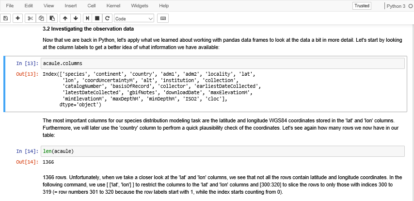
To get a first impression of Jupyter Notebook have a look at Figure 3.2 (which you already saw earlier). The shown excerpt consists of two code cells with Python code (those with starting with “In [...]:“) and the output produced by running the code (“Out[...]:”), and of three different rich text cells before, after, and between the code cells with explanations of what is happening. The currently active cell is marked by the blue bar on the left and frame around it.
Before we continue to discuss what Jupyter Notebook has to offer, let’s get it running on your computer so that you can directly try out the examples.
3.6.1 Running Jupyter Notebook
Juypter Notebook is already installed in the Anaconda environment AC36 or AC37 we created in Section 3.2. If you have the Anaconda Navigator running, make sure it shows the “Home” page and that our AC36 or AC37 environment is selected. Then you should see an entry for Juypter Notebook with a Launch button (Figure 3.3). Click the ‘Launch’ button to start up the application. This will ensure that your notebook starts with the correct environment. Starting Jupyter Notebook this way will create the link to shortcuts for a Jupyter Notebook to that conda environment so you can use it in the way we describe below.

Alternatively, you can start up Jupyter directly without having to open Anaconda first: You will find the Juypter Notebook application in your Windows application list as a subentry of Anaconda. Be sure that you start the Jupyter Notebook for the recently created conda environment (which will only be created if you change the dropdown in Anaconda Navigator above). Alternatively, simply press the Windows key and then type in the first few characters of Jupyter until Jupyter (with the correct conda environment) shows up in the search results.
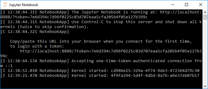
When you start up Jupyter, two things will happen: The server component of the Jupyter application will start up in a Windows command line window showing log messages, e.g. that the server is running locally under the address http://localhost:8888/ (see Figure 3.4 (a)). When you start Jupyter from the Anaconda Navigator, this will actually happen in the background and you won't get to see the command line window with the server messages. In addition, the web-based client application part of Jupyter will open up in your standard web browser showing you the so-called Dashboard, the interface for managing your notebooks, creating new ones, and also managing the kernels. Right now it will show you the content of the default Jupyter home folder, which is your user’s home folder, in a file browser-like interface (Figure 3.4 (b)).
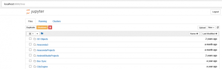
The file tree view allows you to navigate to existing notebooks on your disk, to open them, and to create new ones. Notebook files will have the file extension .ipynb . Let’s start by creating a new notebook file to try out the things shown in the next sections. Click the ‘New…’ button at the top right, then choose the ‘Python 3’ option. A new tab will open up in your browser showing an empty notebook page as in Figure 3.5.
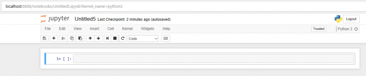
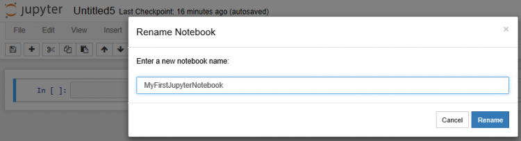
Before we are going to explain how to edit and use the notebook page, please note that the page shows the title of the notebook above a menu bar and a toolbar that provide access to the main operations and settings. Right now, the notebook is still called ‘Untitled...’, so, as a last preparation step, let’s rename the notebook by clicking on the title at the top and typing in ‘MyFirstJupyterNotebook’ as the new title and then clicking the ‘Rename’ button (Figure 3.6).
If you go back to the still open ‘Home’ tab with the file tree view in your browser, you can see your new notebook listed as MyFirstJupyterNotebook.ipynb and with a green ‘Running’ tag indicating that this notebook is currently open. You can also click on the ‘Running’ tab at the top to only see the currently opened notebooks (the ‘Clusters’ tab is not of interest for us at the moment). Since we created this notebook in the Juypter root folder, it will be located directly in your user’s home directory. However, you can move notebook files around in the Windows File Explorer if, for instance, you want the notebook to be in your Documents folder instead. To create a new notebook directly in a subfolder, you would first move to that folder in the file tree view before you click the ‘New…’ button.

3.6.2 First steps to editing a Jupyter Notebook
We will now explain the basics of editing a Jupyter Notebook. We cannot cover all the details here, so if you enjoy working with Jupyter and want to learn all it has to offer as well as all the little tricks that make life easier, the following resources may serve as good starting points:
- Jupyter Documentation [34]
- The Jupyter Notebook [35]
- 28 Jupyter Notebook tips, tricks, and shortcuts [36]
- Jupyter Notebook Tutorial: The Definitive Guide [37]
A Jupyter notebook is always organized as a sequence of so called ‘cells’ with each cell either containing some code or rich text created using the Markdown notation approach (further explained in a moment). The notebook you created in the previous section currently consists of a single empty cell marked by a blue bar on the left that indicates that this is the currently active cell and that you are in ‘Command mode’. When you click into the corresponding text field to add or modify the content of the cell, the bar color will change to green indicating that you are now in ‘Edit mode’. Clicking anywhere outside of the text area of a cell will change back to ‘Command mode’.
Let’s start with a simple example for which we need two cells, the first one with some heading and explaining text and the second one with some simple Python code. To add a second cell, you can simply click on the  symbol. The new cell will be added below the first one and become the new active cell shown by the blue bar (and frame around the cell’s content). In the ‘Insert’ menu at the top, you will also find the option to add a new cell above the currently active one. Both adding a cell above and below the current one can also be done by using the keyboard shortcuts ‘A’ and ‘B’ while in ‘Command mode’. To get an overview on the different keyboard shortcuts, you can use Help -> Keyboard Shortcuts in the menu at the top.
Both cells that we have in our notebook now start with “In [ ]:” in front of the text field for the actual cell content. This indicates that these are ‘Code’ cells, so the content will be interpreted by Jupyter as executable code. To change the type of the first cell to Markdown, select that cell by clicking on it, then change the type from ‘Code’ to ‘Markdown’ in the dropdown menu 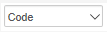 in the toolbar at the top. When you do this, the “In [ ]:” will disappear and your notebook should look similar to Figure 3.8 below. The type of a cell can also be changed by using the keyboard shortcuts ‘Y’ for ‘Code’ and ‘M’ for ‘Markdown’ when in ‘Command mode’.

Let’s start by putting some Python code into the second(!) cell of our notebook. Click on the text field of the second cell so that the bar on the left turns green and you have a blinking cursor at the beginning of the text field. Then enter the following Python code:
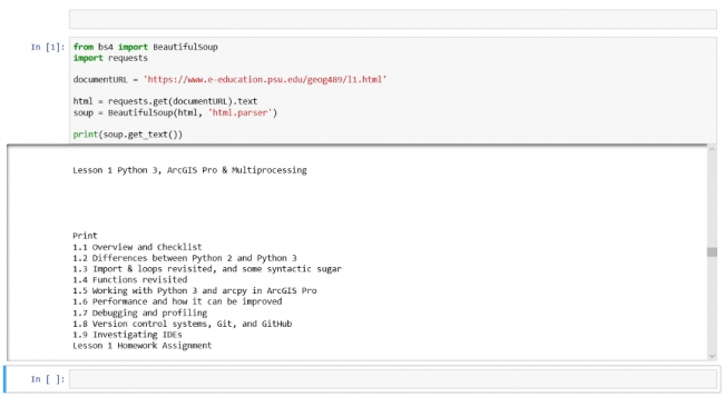
from bs4 import BeautifulSoup
import requests

documentURL = 'https://www.e-education.psu.edu/geog489/l1.html'

html = requests.get(documentURL).text
soup = BeautifulSoup(html, 'html.parser')

print(soup.get_text())
This brief code example is similar to what you already saw in Lesson 2. It uses the requests Python package to read in the content of an html page from the URL that is provided in the documentURL variable. Then the package BeautifulSoup4 (bs4) is used for parsing the content of the file and we simply use it to print out the plain text content with all tags and other elements removed by invoking its get_text() method in the last line.
While Jupyter by default is configured to periodically autosave the notebook, this would be a good point to explicitly save the notebook with the newly added content. You can do this by clicking the disk  symbol or simply pressing ‘S’ while in ‘Command mode’. The time of the last save will be shown at the top of the document, right next to the notebook name. You can always revert back to the last previously saved version (also referred to as a ‘Checkpoint’ in Jupyter) using File -> Revert to Checkpoint. Undo with CTRL-Z works as expected for the content of a cell while in ‘Edit mode’; however, you cannot use it to undo changes made to the structure of the notebook such as moving cells around. A deleted cell can be recovered by pressing ‘Z’ while in ‘Command mode’ though.
Now that we have a cell with some Python code in our notebook, it is time to execute the code and show the output it produces in the notebook. For this you simply have to click the run  symbol button or press ‘SHIFT+Enter’ while in ‘Command mode’. This will execute the currently active cell, place the produced output below the cell, and activate the next cell in the notebook. If there is no next cell (like in our example so far), a new cell will be created. While the code of the cell is being executed, a * will appear within the squared brackets of the “In [ ]:”. Once the execution has terminated, the * will be replaced by a number that always increases by one with each cell execution. This allows for keeping track of the order in which the cells in the notebook have been executed.
Figure 3.9 below shows how things should look after you executed the code cell. The output produced by the print statement is shown below the code in a text field with a vertical scrollbar. We will later see that Jupyter provides the means to display other output than just text, such as images or even interactive maps.
In addition to running just a single cell, there are also options for running all cells in the notebook from beginning to end (Cell -> Run All) or for running all cells from the currently activated one until the end of the notebook (Cell -> Run All Below). The produced output is saved as part of the notebook file, so it will be immediately available when you open the notebook again. You can remove the output for the currently active cell by using Cell -> Current Outputs -> Clear, or of all cells via Cell -> All Output -> Clear.
Let’s now put in some heading and information text into the first cell using the Markdown notation. Markdown [38] is a notation and corresponding conversion tool that allows you to create formatted HTML without having to fiddle with tags and with far less typing required. You see examples of how it works by going Help -> Markdown in the menu bar and then clicking the “Basic writing and formatting syntax” link on the web page that opens up. This page here [39] also provides a very brief overview on the markdown notation. If you browse through the examples, you will see that a first level heading can be produced by starting the line with a hashmark symbol (#). To make some text appear in italics, you can delimit it by * symbols (e.g., *text*), and to make it appear in bold, you would use **text** . A simple bullet point list can be produced by a sequence of lines that start with a – or a *.
Let’s say we just want to provide a title and some bullet point list of what is happening in this code example. Click on the text field of the first cell and then type in:
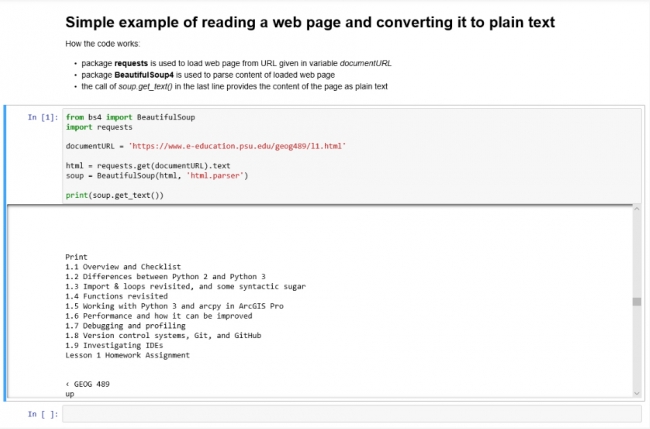
# Simple example of reading a web page and converting it to plain text
How the code works:
* package **requests** is used to load web page from URL given in variable *documentURL*
* package **BeautifulSoup4 (bs4)** is used to parse content of loaded web page
* the call of *soup.get_text()* in the last line provides the content of page as plain text
While typing this in, you will notice that Jupyter already interprets the styling information we are providing with the different notations, e.g. by using a larger blue font for the heading, by using bold font for the text appearing within the **…**, etc. However, to really turn the content into styled text, you will need to ‘run the cell’ (SHIFT+Enter) like you did with the code cell. As a result, you should get the nicely formatted text shown in Figure 3.10 below that depicts our entire first Jupyter notebook with text cell, code cell, and output. If you want to see the Markdown code and edit it again, you will have to double-click the text field or press ‘Enter’ to switch to ‘Edit mode’.
If you have not worked with Markdown styling before, we highly recommend that you take a moment to further explore the different styling options from the “Basic writing and formatting syntax” web page. Either use the first cell of our notebook to try out the different notations or create a new Markdown cell at the bottom of the notebook for experimenting.
This little example only covered the main Jupyter operations needed to create a first Jupyter notebook and run the code in it. The ‘Edit’ menu contains many operations that will be useful when creating more complex notebooks, such as deleting, copying, and moving of cells, splitting and merging functionality, etc. For most of these operations, there also exist keyboard shortcuts. If you find yourself in a situation in which you can’t figure out how to use any of these operations, please feel free to ask on the forums.
3.6.3 Magic commands
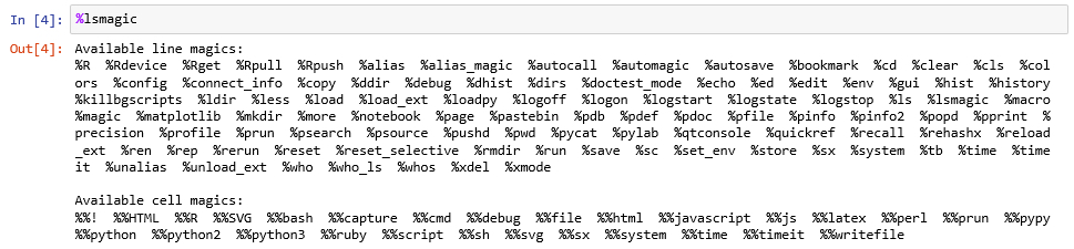
Jupyter provides a number of so-called magic commands that can be used in code cells to simplify common tasks. Magic commands are interpreted by Jupyter and, for instance, transformed into Python code before the content is passed on to the kernel for execution. This happens behind the scenes, so you will always only see the magic command in your notebook. Magic commands start with a single % symbol if they are line-oriented meaning they should be applied to the remaining content of the line, and with %% if they are cell-oriented meaning they should be applied to the rest of the cell. As a first example, you can use the magic command %lsmagic to list the available magic commands (Figure 3.11). To get the output you have to execute the cell as with any other code cell.
The %load_ext magic command can be used for loading IPython extension which can add new magic commands. The following command loads the IPython rpy2 extension. If that code gives you a long list of errors then the rpy2 package isn't installed and you will need to go back to Section 3.2 and follow the instructions there.
We recently had cases where loading rpy2 failed on some systems due to the R_HOME environment variable not being set correctly. We therefore added the first line below which you will have to adapt to point to the lib\R folder in your AC Python environment.
import os, rpy2
os.environ['R_HOME'] = r'C:\Users\username\anaconda3\envs\AC37\lib\R' # workaround for R.dll issue occurring on some systems
%load_ext rpy2.ipython
Using a ? symbol in front of a magic command will open a subwindow with the documentation of that command at the bottom of the browser window. Give it a try by executing the command
?%Rin a cell. %R is a magic command from the rpy2 extension that we just loaded and the documentation will tell you that this command can be used to execute some line of R code that follows the %R and optionally pass variable values between the Python and R environments. We will use this command several times in the lesson’s walkthrough to bridge between Python and R. Keep in mind that it is just an abbreviation that will be replaced with a bunch of Python statements by Jupyter. If you would want the same code to work as a stand-alone Python script outside of Jupyter, you would have to replace the magic command by these Python statements yourself. You can also use the ? prefix to show the documentation of Python elements such as classes and functions, for instance by writing
?BeautifulSoup
or
?soup.get_text()
Give it a try and see if you understand what the documentation is telling you.
3.6.4 Widgets
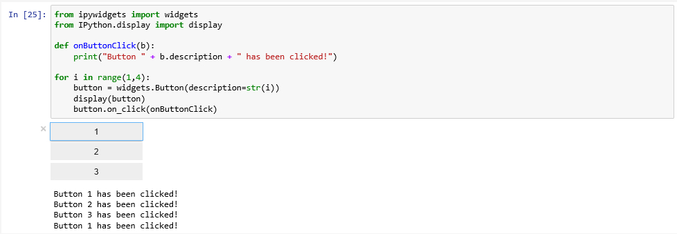
Jupyter notebooks can also include interactive elements, referred to as widgets as in Lesson 2, like buttons, text input fields, sliders, and other GUI elements, as well as visualizations, plots, and animations. Figure 3.12 shows an example that places three button widgets and then simply prints out which button has been pressed when you click on them. The ipywidgets and IPython.display packages imported at the beginning are the main packages required to place the widgets in the notebook. We then define a function that will be invoked whenever one of the buttons is clicked. It simply prints out the description attribute of the button (b.description). In the for-loop we create the three buttons and register the onButtonClick function as the on_click event handler function for all of them.
from ipywidgets import widgets
from IPython.display import display

def onButtonClick(b):
    print("Button " + b.description + " has been clicked")

for i in range(1,4):
    button = widgets.Button(description=str(i))
    display(button)
    button.on_click(onButtonClick)
If you get an error with this code "Failed to display Jupyter Widget of type Button" that means the widgets are probably not installed which we can potentially fix in our Anaconda prompt:
conda install -n base -c conda-forge widgetsnbextension
conda install -n AC37 -c conda-forge ipywidgets
After installing the packages, exit your Jupyter notebook and restart it and try to re-run your code. It's possible you will receive the error again as the widget tries to run before the Javascript library that runs the widgets has opened. In that case try to select your code, wait a few more seconds and then click Run.
If you're still getting an error, it's likely that your packages didn't install properly (or in a way that Jupyter/Anaconda could find them). The fix for this is to close Jupyter Notebook, return to Anaconda Navigator, click Environments (on the left), choose your environment and then search for "ipy", you may need to either change the "Installed" dropdown to "Not Installed" if they are missing or perhaps they should be updated (by clicking on the upward point arrow or the blue text).
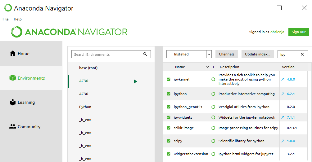
It is easy to imagine how this example could be extended to provide some choices on how the next analysis step in a longer Data Science project should be performed. Similarly, a slider or text input field could be used to allow the notebook user to change the values of important input variables.
3.6.5 Autocompletion, restarting the kernel, and other useful things
Let’s close this brief introduction to Jupyter with a few more things that are good to know when starting to write longer and more complex notebooks. Like normal development environments, Juypter has an autocomplete feature that helps with the code writing and can save a lot of typing: while editing code in a code cell, you can press the TAB key and Jupyter will either automatically complement the name or keyword you are writing or provide you with a dropdown list of choices that you can pick from. For instance, type in soup.ge and then press TAB and you get the list of options, as shown in Figure 3.13 including the get_text() function that we used in our code.
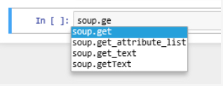
Another useful keyboard command to remember is SHIFT+TAB. When you place the cursor on a variable name or function call and press this key combination, a window will open up showing helpful information like the type of the variable and its current content or the parameters of the function as in Figure 3.14. This is of great help if you are unsure about the different parameters of a function, their order or names. Try out what you get when you use this key combination for different parts of the code in this notebook.
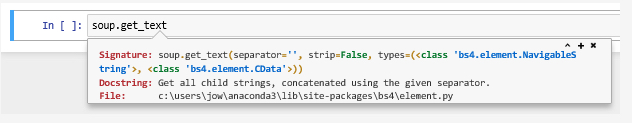
As in all programming, it may occasionally happen that something goes completely wrong and the execution of the code in a cell won’t terminate in the expected time or not at all. If that happens, the first thing to try is to use the “Interrupt Kernel” button located to the right of the “Execute cell” button. This should stop the execution of the current cell and you can then modify the code and try to run the cell again. However, sometimes even that won’t help because the kernel has become unresponsive. In that case, the only thing you can do is restart the kernel using the “Restart Kernel” button to the right of the “Interrupt Kernel” button. Unfortunately, that means that you will have to start the execution of the code in your notebook from the beginning because all imports and variable assignments will be lost after the restart.
Once you have finished your notebook, you may want to publish or share it. There are many options by wich to do so. In the File menu, there exists the “Download as…” option for obtaining versions of your notebook in different formats. The .ipynb format, as we mentioned, is the native format in which Jupyter saves the notebooks. If you make the .ipynb file available to someone who has access to Juypter, that person can open the notebook and run it or modify the content. The .py option allows for exporting content as a Python script, so that the code can be run outside of Jupyter. If you want a version of your notebook that others can read even without access to Jupyter, there are several options like exporting the notebook as HTML, as Latex, or as PDF. Some of these options require additional software tools to be installed on your computer and there are some limitations. For instance, if you export your notebook as HTML to add it to your personal web page, interactive widgets such as the interactive web map you will see later in Section 3.10 will not be included.
To close this section, we want to again refer to the links we provided at the beginning of Section 3.6.2 if you want to keep reading about Jupyter and learn tricks that we weren't able to cover in this brief introduction. In the remainder of this lesson, please use Jupyter to try out the code examples by entering them into a Jupyter notebook and running the code there to get some more practice with Jupyter.
3.7 Species distribution modeling with R and the dismo package
Before we will start to create another Jupyter notebook with a much more complex example, let us talk about the task and application domain we will be using. As we mentioned at the beginning of the lesson, we will be using a Jupyter notebook to connect Python with R to be able to use some specialized statistical models for the application field of species distribution modeling.
Simply speaking, species distribution modeling is the task or process of predicting the real-world distribution or likelihood of a species occurring at any location on the earth based on (a) existing occurrence and potentially also absence data, e.g. from biological surveys, and (b) data for a number of predictive variables, most often climate related, but also including elevation, soil type, land cover type, etc. The output of a species distribution model is typically a raster with probabilities for the area of interest (which might be the entire earth) that can be used to create a map visualization to help with analysis and decision making. Anticipating the main result of this lesson’s walkthrough, Figure 3.15(b) shows the distribution of Solanum acaule, a plant species growing in the western countries of South America, as predicted by a particular species distribution model that is implemented in the R package ‘dismo’ developed and maintained by Robert J. Hijmans and colleagues. The prediction has been created with the Bioclim model which is one of several models available in dismo.

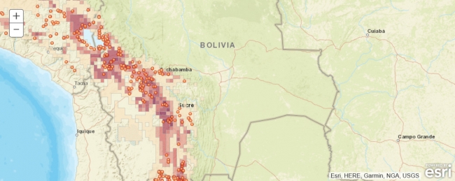
Teaching you the basics of R is beyond the scope of this course, and you really won’t need R knowledge to follow and understand the short pieces of R code we will be using in this lesson’s walkthrough. However, if you have not worked with R before, you may want to take a quick look through the first five sections of this brief R tutorial [40] (or one of the many other R tutorials on the web). Please note that in this lesson we are not trying to create the best possible distribution model for Solanum acaule (and what actually makes a good or optimal model is something that is heavily debated even among experts anyway). Our main goal is to introduce different Python packages and show how they can be combined to solve spatial analysis tasks inside a Jupyter notebook without letting things get too complex. We, therefore, made quite a few simplifications with regard to what input data to use, how to preprocess it, the species distribution model itself, and how it is applied. As a result, the final model created and shown in the figure above should be taken with a grain of salt.
The ‘dismo’ R package contains a collection of different species modeling approaches as well as many auxiliary functions for obtaining and preprocessing data. See the official documentation of the module [41]. The authors have published detailed additional documentation available in this species distribution modeling document [42] that provides examples and application guidelines for the package and that served as a direct inspiration for this lesson’s walkthrough. One of the main differences is that we will be doing most of the work in Python and only use R and the ‘dismo’ package to obtain some part of the input data and later apply a particular species modeling approach to this data.
Species distribution modeling approaches can roughly be categorized into methods that only use presence data and methods that use both presence and absence data as well as into regression and machine learning based methods. The ‘dismo’ package provides implementations of various models from these different classes but we will only use a rather simple one, the Bioclim model, in this lesson. Bioclim only uses presence data and looks at how close the values of given environmental predictor variables (provided as raster files) for a particular location are to the median values of these variables over the locations where the species has been observed. Because of its simplicity, Bioclim is particularly well suited for teaching purposes.
The creation of a prediction typically consists of the following steps:
- Obtaining and preprocessing of all input data (species presence/absence data and data for environmental predictor variables)
- Creation of the model from the input data
- Using the model to create a prediction based on data for the predictor variables.
require('dismo')
bc <- bioclim(predictorRasters, observationPoints)
You can then use the model to create a Bioclim prediction raster and store it in variable pb and create a plot of the raster with the following R code:
pb <- predict(predictorRasters, bc)
plot(pb, main='Bioclim, raw values')
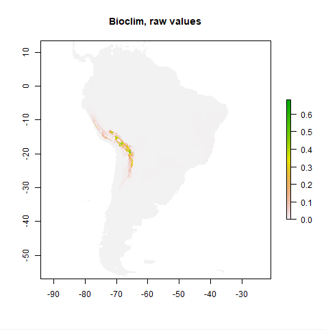
You may be wondering how you can actually use R commands from inside your Python code. We already mentioned that the magic command %R (or %%R for the cell-oriented version) can be used to invoke R commands within a Python Jupyter notebook. The connection via Python and R is implemented by the rpy2 package [43] that allows for running R inside a Python process. We cannot go into the details of how rpy2 works and how one would use it outside of Jupyter here, so we will just focus on the usage via the %R magic command. To prepare your Jupyter Notebook to interface with R, you will always first have to run the magic command
%load_ext rpy2.ipython
... to load the IPhython rpy2 extension. (If you are trying this out and get an error message about being unable to load the R.dll library, use the following command to manually define the R_HOME environment variable, put in your Windows user ID, and make sure it points to the R folder in your Anaconda AC36/37 environment: os.environ['R_HOME'] = r'C:\Users\youruserid\anaconda3\envs\AC37\lib\R' )
We can then simply execute a single R command by using
%R <command>
To transfer the content of a Python variable to R, we can use
%R –i <name of Python variable>
This creates an R variable with the same name as the Python variable and an R version of the content assigned to it. Similarly,
%R –o <name of R variable>
...can be used for the other direction, so for creating a Python variable with the same name and content as a given R variable. As we will further see in the lesson’s walkthrough, these steps combined make it easy to use R inside a Python Jupyter notebook. However, one additional important component is needed: in R most data used comes in the form of so-called data frames, spreadsheet-like data objects in tabular form in which the content is structured into rows, columns, and cells. R provides a huge collection of operations to read, write, and manipulate data frames. Can we find something similar on the Python side as well that will allow us to work with tabular data (such as attribute information for a set of spatial features) directly in Python? The answer is yes, and the commonly used package to work with tabular data in Python is pandas, so we will talk about it next.
3.8 Pandas and the manipulation of tabular data
The pandas package provides high-performance data structures and analysis tools, in particular for working with tabular data based on a fast and efficient implementation of a data frame class. It also allows for reading and writing data from/to various formats including CSV and Microsoft Excel. In the following, we show you some examples illustrating how to perform the most important data frame related operations with pandas. Again, we can only scratch the surface of the functionality provided by pandas here. Resources provided at the end will allow you to dive deeper if you wish to do so. We recommend that you start a new Jupyter Notebook and use it to try out the examples from this section for yourself. Use a new code cell for each of block of code you will encounter on the following pages.
3.8.1 Creating a new data frame
In our examples, we will be using pandas in combination with the numpy package, the package that provides many fundamental scientific computing functionalities for Python and that many other packages are built on. So we start by importing both packages:
import pandas as pd
import numpy as np
A data frame consists of cells that are organized into rows and columns. The rows and columns have names that serve as indices to access the data in the cells. Let us start by creating a data frame with some random numbers that simulate a time series of different measurements (columns) taken on consecutive days (rows) from January 1, 2017 to January 6, 2017. The first step is to create a pandas series of dates that will serve as the row names for our data frame. For this, we use the pandas function date_range(…):
dates = pd.date_range('20170101' , periods=6, freq='D')
dates
The first parameter given to date_range is the starting date. The ‘periods’ parameter tells the function how many dates we want to generate, while we use ‘freq’ to tell it that we want a date for every consecutive day. If you look at the output from the second line we included, you will see that the object returned by the function is a DatetimeIndex object which is a special class defined in pandas.
Next, we generate random numbers that should make up the content of our date frame with the help of the numpy function randn(…) for creating a set of random numbers that follow a standard normal distribution:
numbers = np.random.randn(6,4)
numbers
The output is a two-dimensional numpy array of random numbers normally distributed around 0 with 4 columns and 6 rows. We create a pandas data frame object from it with the following code:
df = pd.DataFrame(numbers, index=dates, columns=['m1', 'm2', 'm3', 'm4'])
df
Note that we provide our array of random numbers as the first parameter, followed by the DatetimeIndex object we created earlier for the row index. For the columns, we simply provide a list of the names with ‘m1’ standing for measurement 1, ‘m2’ standing for measurement 2, and so on. Please also note how the resulting data frame is displayed as a nicely formatted table in your Jupyter Notebook because it makes use of IPython widgets. Please keep in mind that because we are using random numbers for the content of the cells, the output produced by commands used in the following examples will look different in your notebook because the numbers are different.
3.8.2 Subsetting and changing cell values
Now that we have a data frame object available, let’s quickly go through some of the basic operations that one can perform on a data frame to access or modify the data.
The info() method can be used to display some basic information about a data frame such as the number of rows and columns and data types of the columns:
df.info()
The output tells us that we have four columns, all for storing floating point numbers, and each column has 6 rows with values that are not null. If you ever need the number of rows and columns, you can get them by applying the len(…) operation to the data frame and to the columns property of the data frame:
print(len(df))          # gives you the number of rows
print(len(df.columns))  # gives you the number of columns
We can use the head(…) and tail(…) methods to get only the first or last n rows of a data frame:
firstRows = df.head(2)
print(firstRows)
lastRows = df.tail(2)
print(lastRows)
We can also just get a subset of consecutive rows by applying slicing to the data frame similar to how this can be done with lists or strings:
someRows = df[3:5]    # gives you the 4th and 5th row
print(someRows)
This operation gives us rows 4 and 5 (those with index 3 and 4) from the original data frame because the second number used is the index of the first row that will not be included anymore.
If we are just interested in a single column, we can get it based on its name:
thirdColumn = df.m3
print(thirdColumn)
The same can be achieved by using the notation df['m3'] instead of df.m3 in the first line of code. Moreover, instead of using a single column name, you can use a list of column names to get a data frame with just these columns and in the specified order:
columnsM3andM2 = df[ ['m3', 'm2'] ]
columnsM3andM2
| m3 | m2 | |
|---|---|---|
| 2017-01-01 | 0.510162 | 0.163613 |
| 2017-01-02 | 0.025050 | 0.056027 |
| 2017-01-03 | -0.422343 | -0.840010 |
| 2017-01-04 | -0.966351 | -0.721431 |
| 2017-01-05 | -1.339799 | 0.655267 |
| 2017-01-06 | -1.160902 | 0.192804 |
The column subsetting and row slicing operations shown above can be concatenated into a single expression. For instance, the following command gives us columns ‘m3’ and ‘m2’ and only the rows with index 3 and 4:
someSubset = df[['m3', 'm2']][3:5]
someSubset
The order here doesn’t matter. We could also have written df[3:5][['m3', 'm2']] .
The most flexible methods for creating subsets of data frame are via the loc and .iloc index properties of a data frame. .iloc[…] is based on the numerical indices of the columns and rows. Here is an example:
someSubset = df.iloc[2:4,1:3]
print(someSubset)
The part before the comma determines the rows (rows with indices 2 and 3 in this case) and the part after the comma, the columns (columns with indices 1 and 2 in this case). So we get a data frame with the 3rd and 4th rows and 2nd and 3rd columns of the original data frame. Instead of slices we can also use lists of row and column indices to create completely arbitrary subsets. For instance, using iloc in the following example
someSubset = df.iloc[ [0,2,4], [1,3] ]
print(someSubset)
...gives us a data frame with the 1st, 3rd, and 5th row and 2nd and 4th column of the original dataframe. Both the part before the comma and after the comma can just be a colon symbol (:) in which case all rows/columns will be included. For instance,
allRowsSomeColumns = df.iloc[ : , [1,3] ]
print(allRowsSomeColumns)
...will give you all rows but only the 2nd of 4th column.
In contrast to iloc, loc doesn’t use the row and column numbers but instead is based on their labels, while otherwise working in the same way as iloc. The following command produces the same subset of the 1st, 3rd, and 5th rows and 2nd and 4th columns as the iloc code from two examples above:
someSubset = df.loc[ [pd.Timestamp('2017-01-01'), pd.Timestamp('2017-01-03'), pd.Timestamp('2017-01-05')] , ['m2', 'm4'] ]
print(someSubset)
Please note that, in this example, the list for the column names at the very end is simply a list of strings but the list of dates for the row names has to consist of pandas Timestamp objects. That is because we used a DatetimeIndex for the rows when we created the original data frame. When a data frame is displayed, the row names show up as simple strings but they are actually Timestamp objects. However, a DatetimeIndex for the rows has many advantages; for instance, we can use it to get all rows for dates that are from a particular year, e.g. with
df.loc['2017' , ['m2', 'm4'] ]
...to get all dates from 2017 which, of course, in this case, are all rows. Without going into further detail here, we can also get all dates from a specified time period, etc.
The methods explained above for accessing subsets of a data frame can also be used as part of an assignment to change the values in one or several cells. In the simplest case, we can change the value in a single cell, for instance with
df.iloc[0,0] = 0.17
...or
df.loc['2017-01-01', 'm1'] = 0.17
...to change the value of the top left cell to 0.17. Please note that this operation will change the original data frame, not create a modified copy. So if you now print out the data frame with
df
you will see the modified value for 'm1' of January 1, 2017. Even more importantly, if you have used the operations explained above for creating a subset, the data frame with the subset will still refer to the original data, so changing a cell value will change your original data. If you ever want to make changes but keep the original data frame unchanged, you need to explicitly make a copy of the data frame by calling the copy() method as in the following example:
dfCopy = df.copy()
dfCopy.iloc[0,0] = 0
print(df)
print(dfCopy)
Check out the output and compare the top left value for both data frames. The data frame in df still has the old value of 0.17, while the value will be changed to 0 in dfCopy. Without using the copy() method in the first line, both variables would still refer to the same underlying data and both would show the 0 value. Here is another slightly more complicated example where we change the values for the first column of the 1st and 5th rows to 1.2 (intentionally modifying the original data):
df.iloc[ [0,4] , [0] ] = 1.2
print(df)
If you ever need to explicitly go through the rows in a data frame, you can do this with a for-loop that uses the itertuples(…) method of the data frame. itertuples(…) gives you an object that can be used to iterate through the rows as named tuples, meaning each element in the tuple is labeled with the respective column name. By providing the parameter index=False to the method, we are saying that we don’t want the row name to be part of the tuple, just the cell values for the different columns. You can access the elements of the tuple either via their index or via the column name:
for row in df.itertuples(index=False):
    print(row)     # print entire row tuple
    print(row[0])  # print value from column with index 0
    print(row.m2)  # print value from column with name m2
    print('----------')
Try out this example and have a look at the named tuple and the output produced by the other two print statements.
3.8.3 Sorting
Pandas also provides operations for sorting the rows in a data frame. The following command can be used to sort our data frame by the values in the ‘m2’ column in decreasing order:
dfSorted = df.sort_values(by='m2', ascending=False)
dfSorted
| m1 | m2 | m3 | m4 | m5 | |
|---|---|---|---|---|---|
| 2017-01-05 | 1.200000 | 0.655267 | -1.339799 | 1.075069 | -0.236980 |
| 2017-01-06 | 0.192804 | 0.192804 | -1.160902 | 0.525051 | -0.412310 |
| 2017-01-01 | 1.200000 | 0.163613 | 0.510162 | 0.628612 | 0.432523 |
| 2017-01-02 | 0.056027 | 0.056027 | 0.025050 | 0.283586 | -0.123223 |
| 2017-01-04 | -0.721431 | -0.721431 | -0.966351 | -0.380911 | 0.001231 |
| 2017-01-03 | -0.840010 | -0.840010 | -0.422343 | 1.022622 | -0.231232 |
The ‘by’ argument specifies the column that the sorting should be based on and, by setting the ‘ascending’ argument to False, we are saying that we want the rows to be sorted in descending rather than ascending order. It is also possible to provide a list of column names for the ‘by’ argument, to sort by multiple columns. The sort_values(...) method will create a new copy of the data frame, so modifying any cells of dfSorted in this example will not have any impact on the data frame in variable df.
3.8.4 Adding / removing columns and rows
Adding a new column to a data frame is very simple when you have the values for that column ready in a list. For instance, in the following example, we want to add a new column ‘m5’ with additional measurements and we already have the numbers stored in a list m5values that is defined in the first line of the example code. To add the column, we then simply make an assignment to df['m5'] in the second line. If a column ‘m5’ would already exist, its values would now be overwritten by the values from m5values. But since this is not the case, a new column gets added under the name ‘m5’ with the values from m5values.
m5values = [0.432523, -0.123223, -0.231232, 0.001231, -0.23698, -0.41231]
df['m5'] = m5values
df
| m1 | m2 | m3 | m4 | m5 | |
|---|---|---|---|---|---|
| 2017-01-01 | 1.200000 | 0.163613 | 0.510162 | 0.628612 | 0.432523 |
| 2017-01-02 | 0.056027 | 0.056027 | 0.025050 | 0.283586 | -0.123223 |
| 2017-01-03 | -0.840010 | -0.840010 | -0.422343 | 1.022622 | -0.231232 |
| 2017-01-04 | -0.721431 | -0.721431 | -0.966351 | -0.380911 | 0.001231 |
| 2017-01-05 | 1.200000 | 0.655267 | -1.339799 | 1.075069 | -0.236980 |
| 2017-01-06 | 0.192804 | 0.192804 | -1.160902 | 0.525051 | -0.412310 |
For adding new rows, we can simply make assignments to the rows selected via the loc operation, e.g. we could add a new row for January 7, 2017 by writing
df.loc[pd.Timestamp('2017-01-07'),:] = [ ... ]
where the part after the equal sign is a list of five numbers, one for each of the columns. Again, this would replace the values in the case that there already is a row for January 7. The following example uses this idea to create new rows for January 7 to 9 using a for loop:
for i in range(7,10):
    df.loc[ pd.Timestamp('2017-01-0'+str(i)),:] = [ np.random.rand() for j in range(5) ]
df
| m1 | m2 | m3 | m4 | m5 | |
|---|---|---|---|---|---|
| 2017-01-01 | 1.200000 | 0.163613 | 0.510162 | 0.628612 | 0.432523 |
| 2017-01-02 | 0.056027 | 0.056027 | 0.025050 | 0.283586 | -0.123223 |
| 2017-01-03 | -0.840010 | -0.840010 | -0.422343 | 1.022622 | -0.231232 |
| 2017-01-04 | -0.721431 | -0.721431 | -0.966351 | -0.380911 | 0.001231 |
| 2017-01-05 | 1.200000 | 0.655267 | -1.339799 | 1.075069 | -0.236980 |
| 2017-01-06 | 0.192804 | 0.192804 | -1.160902 | 0.525051 | -0.412310 |
| 2017-01-07 | 0.768633 | 0.559968 | 0.591466 | 0.210762 | 0.610931 |
| 2017-01-08 | 0.483585 | 0.652091 | 0.183052 | 0.278018 | 0.858656 |
| 2017-01-09 | 0.909180 | 0.917903 | 0.226194 | 0.978862 | 0.751596 |
In the body of the for loop, the part on the left of the equal sign uses loc(...) to refer to a row for the new date based on loop variable i, while the part on the right side simply uses the numpy rand() method inside a list comprehension to create a list of five random numbers that will be assigned to the cells of the new row.
If you ever want to remove columns or rows from a data frame, you can do so by using df.drop(...). The first parameter given to drop(...) is a single column or row name or, alternatively, a list of names that should be dropped. By default, drop(...) will consider these as row names. To indicate these are column names that should be removed, you have to specify the additional keyword argument axis=1 . We will see an example of this in a moment.
3.8.5 Joining data frames
The following short example demonstrates how pandas can be used to merge two data frames based on a common key, so to perform a join operation in database terms. Let’s say we have two tables, one listing capitals of states in the U.S. and one listing populations for each state. For simplicity we just define data frames for these with just entries for two states, Washington and Oregon:
df1 = pd.DataFrame( {'state': ['Washington', 'Oregon'], 'capital': ['Olympia', 'Salem']} )
print(df1)
df2 = pd.DataFrame( {'name': ['Washington', 'Oregon'], 'population':[7288000, 4093000]} )
print(df2)
The two data frames produced by this code look like this:
| capital | state | |
|---|---|---|
| 0 | Olympia | Washington |
| 1 | Salem | Oregon |
| name | population | |
|---|---|---|
| 0 | Washington | 7288000 |
| 1 | Oregon | 4093000 |
We here use a new way of creating a data frame, namely from a dictionary that has entries for each of the columns where the keys are the column names (‘state’ and ‘capital’ in the case of df1, and ‘name’ and ‘population’ in case of df2) and the values stored are lists of the values for that column. We now invoke the merge(...) method on df1 and provide df2 as the first parameter meaning that a new data frame will be produced by merging df1 and df2. We further have to specify which columns should be used as keys for the join operation. Since the two columns containing the state names are called differently, we have to provide the name for df1 through the ‘left_on’ argument and the name for df2 through the ‘right_on’ argument.
merged = df1.merge(df2, left_on='state', right_on='name')
merged
The joined data frame produced by the code will look like this:
| capital | state | name | population | |
|---|---|---|---|---|
| 0 | Olympia | Washington | Washington | 7288000 |
| 1 | Salem | Oregon | Oregon | 4093000 |
As you see, the data frames have been merged correctly. However, we do not want two columns with the state names, so, as a last step, we remove the column called ‘name’ with the previously mentioned drop(...) method. As explained, we have to use the keyword argument axis=1 to indicate that we want to drop a column, not a row.
newMerged = merged.drop('name', axis=1)
newMerged
Result:
| capital | state | population | |
|---|---|---|---|
| 0 | Olympia | Washington | 7288000 |
| 1 | Salem | Oregon | 4093000 |
If you print out variable merged, you will see that it still contains the 'name' column. That is because drop(...) doesn't change the original data frame but rather produces a copy with the column/row removed.
3.8.6 Advanced data frame manipulation: Filtering via Boolean indexing
When working with tabular data, it is very common that one wants to do something with particular data entries that satisfy a certain condition. For instance, we may want to restrict our analysis to rows that have a value larger than a given threshold for one of the columns. Pandas provides some powerful methods for this kind of filtering, and we are going to show one of these to you in this section, namely filtering with Boolean expressions.
The first important thing to know is that we can use data frames in comparison expressions, like df > 0, df.m1 * 2 < 0.2, and so on. The output will be a data frame that only contains Boolean values (True or False) indicating whether the corresponding cell values satisfy the comparison expression or not. Let’s try out these two examples:
df > 0
The result is a data frame with the same rows and columns as the original data frame in df with all cells that had a value larger than 0 set to True, while all other cells are set to False:
| m1 | m2 | m3 | m4 | m5 | |
|---|---|---|---|---|---|
| 2017-01-01 | True | True | True | True | True |
| 2017-01-02 | True | True | True | True | False |
| 2017-01-03 | False | False | False | False | False |
| 2017-01-04 | False | False | False | False | True |
| 2017-01-05 | True | True | False | True | False |
| 2017-01-06 | True | True | False | True | False |
| 2017-01-07 | True | True | True | True | True |
| 2017-01-08 | True | True | True | True | True |
| 2017-01-09 | True | True | True | True | True |
df.m1 * 2 < 0.2
Here we are doing pretty much the same thing but only for a single column (‘m1’) and the comparison expression is slightly more complex involving multiplication of the cell values with 2 before the result is compared to 0.2. The result is a one-dimensional vector of True and False values corresponding to the cells of the ‘m1’ column in the original data frame:
| 2017-01-01 | False |
|---|---|
| 2017-01-02 | True |
| 2017-01-03 | True |
| 2017-01-04 | True |
| 2017-01-05 | False |
| 2017-01-06 | False |
| 2017-01-07 | False |
| 2017-01-08 | True |
| 2017-01-09 | True |
| Freq: D, Name: m1, dtype: bool | |
Just to introduce another useful pandas method, we can apply the value_counts() method to get a summary of the values in a data frame telling how often each value occurs:
(df.m1 * 2 < 0.2).value_counts()
The expression in the parentheses will give us a boolean column vector as we have seen above, and invoking its value_counts() method tells us how often True and False occur in this vector. (The actual numbers will depend on the random numbers in your original data frame).
The second important component of Boolean indexing is that we can use Boolean operators to combine Boolean data frames as illustrated in the next example:
v1 = df.m1 * 2 < 0.2
print(v1)
v2 = df.m2 > 0
print(v2)
print(~v1)
print(v1 & v2)
print(v1 | v2)
This will produce the following output data frames:
| 2017-01-01 | False |
|---|---|
| 2017-01-02 | True |
| 2017-01-03 | True |
| 2017-01-04 | True |
| 2017-01-05 | False |
| 2017-01-06 | False |
| 2017-01-07 | False |
| 2017-01-08 | True |
| 2017-01-09 | True |
| Frew: D, Name: m1, dtype: bool | |
| 2017-01-01 | True |
|---|---|
| 2017-01-02 | False |
| 2017-01-03 | False |
| 2017-01-04 | True |
| 2017-01-05 | True |
| 2017-01-06 | True |
| 2017-01-07 | True |
| 2017-01-08 | True |
| 2017-01-09 | True |
| Frew: D, Name: m2, dtype: bool | |
| 2017-01-01 | True |
|---|---|
| 2017-01-02 | False |
| 2017-01-03 | False |
| 2017-01-04 | False |
| 2017-01-05 | True |
| 2017-01-06 | True |
| 2017-01-07 | True |
| 2017-01-08 | False |
| 2017-01-09 | False |
| Frew: D, Name: m1, dtype: bool | |
| 2017-01-01 | False |
|---|---|
| 2017-01-02 | True |
| 2017-01-03 | False |
| 2017-01-04 | False |
| 2017-01-05 | False |
| 2017-01-06 | False |
| 2017-01-07 | False |
| 2017-01-08 | True |
| 2017-01-09 | True |
| Frew: D, dtype: bool | |
| 2017-01-01 | True |
|---|---|
| 2017-01-02 | True |
| 2017-01-03 | True |
| 2017-01-04 | True |
| 2017-01-05 | True |
| 2017-01-06 | True |
| 2017-01-07 | True |
| 2017-01-08 | True |
| 2017-01-09 | True |
| Frew: D, dtype: bool | |
What is happening here? We first create two different Boolean vectors using two different comparison expressions for columns ‘m1’ and ‘m2’, respectively, and store the results in variables v1 and v2. Then we use the Boolean operators ~ (not), & (and), and | (or) to create new Boolean vectors from the original ones, first by negating the Boolean values from v1, then by taking the logical AND of the corresponding values in v1 and v2 (meaning only cells that have True for both v1 and v2 will be set to True in the resulting vector), and finally by doing the same but with the logical OR (meaning only cells that have False for both v1 and v2 will be set to False in the result). We can construct arbitrarily complex Boolean expressions over the values in one or multiple data frames in this way.
The final important component is that we can use Boolean vectors or lists to select rows from a data frame. For instance,
df[ [True, False, True, False, True, False, True, False, True] ]
... will give us a subset of the data frame with only every second row:
| m1 | m2 | m3 | m4 | m5 | |
|---|---|---|---|---|---|
| 2017-01-01 | 1.200000 | 0.163613 | 0.510162 | 0.628612 | 0.432523 |
| 2017-01-03 | -0.840010 | -0.840010 | -0.422343 | 1.022622 | -0.231232 |
| 2017-01-05 | 1.200000 | 0.655267 | -1.339799 | 1.075069 | -0.236980 |
| 2017-01-07 | 0.399069 | 0.029156 | 0.937808 | 0.476401 | 0.766952 |
| 2017-01-09 | 0.041115 | 0.984202 | 0.912212 | 0.740345 | 0.148835 |
Taken these three things together means we can use arbitrarily logical expressions over the values in a data frame to select a subset of rows that we want to work with. To continue the examples from above, let’s say that we want only those rows that satisfy both the criteria df.m1 * 2 < 0.2 and df.m2 > 0, so only those rows for which the value of column ‘m1’ times 2 is smaller than 0.2 and the value of column ‘m2’ is larger than 0. We can use the following expression for this:
df[v1 & v2 ]
Or even without first having to define v1 and v2:
df[ (df.m1 * 2 < 0.2) & (df.m2 > 0) ]
Here is the resulting data frame:
| m1 | m2 | m3 | m4 | m5 | |
|---|---|---|---|---|---|
| 2017-01-02 | 0.056027 | 0.056027 | 0.025050 | 0.283586 | -0.123223 |
| 2017-01-08 | 0.043226 | 0.904844 | 0.181999 | 0.253381 | 0.165105 |
| 2017-01-09 | 0.041115 | 0.984202 | 0.912212 | 0.740345 | 0.148835 |
Hopefully you are beginning to see how powerful this approach is and how it allows for writing very elegant and compact code for working with tabular data. You will get to see more examples of this and of using pandas in general in the lesson’s walkthrough. There we will also be using GeoPandas, an extension built on top of pandas that allows for working with data frames that contain geometry data, e.g. entire attribute tables of an ESRI shapefile.
3.9 GDAL/OGR
After this general introduction to pandas, we come back to the geospatial domain and will talk about GDAL/OGR [44] a bit. GDAL is a raster and vector processing library that has been developed with a strong focus on supporting a large number of file formats, being able to translate between the different formats, and fostering data exchange. As we already mentioned, GDAL and OGR were originally two separate libraries focusing on raster data (GDAL) and vector data (OGR), respectively. These have now been merged and GDAL (‘Geospatial Data Abstraction Library’) is commonly used to refer to the combined library.
GDAL had its initial release in the year 2000 and originally was mainly developed by Frank Warmerdam. But, since version 1.3.2, responsibilities have been handed over to the GDAL/OGR Project Management Committee under the umbrella of the Open Source Geospatial Foundation [45] (OSGeo). GDAL is available under the permissiveX/MIT style free software license and has become one of the major open source GIS libraries, used in many open source GIS software, including QGIS. The GDAL Python package provides a wrapper around the GDAL C++ library that allows for using its functionality in Python. Similar support exists for other languages and it is also possible to use GDAL/OGR commands from the command line of your operating system. The classes and functions of the Python package are documented here [33]. In the following, we show a few examples illustrating common patterns of using the GDAL library with Python.
3.9.1 Working with vector data
OGR and GDAL exist as separate modules in the osgeo package together with some other modules such as OSR for dealing with different projections and some auxiliary modules. As with previous packages you will probably need to install gdal (which encapsulates all of them in its latest release) to access these packages. So typically, a Python project using GDAL would import the needed modules similar to this:
from osgeo import gdal
from osgeo import ogr
from osgeo import osr
Let’s start with taking a closer look at the ogr module for working with vector data. The following code, for instance, illustrates how one would open an existing vector data set, in this case an Esri shapefile. OGR uses so-called drivers to access files in different formats, so the important thing to note is how we first obtain a driver object for ‘ESRI Shapefile’ with GetDriverByName(...) and then use that to open the shapefile with the Open(...) method of the driver object. The shapefile we are using in this example is a file with polygons for all countries in the world (available here) [46] and we will use it again in the lesson’s walkthrough. When you download it, you may still have to adapt the path in the first line of the code below.
shapefile = r'C:\489\L3\TM_WORLD_BORDERS-0.3.shp'
drv =ogr.GetDriverByName('ESRI Shapefile')
dataSet = drv.Open(shapefile)
dataSet now provides access to the data in the shapefile as layers, in this case just a single layer, that can be accessed with the GetLayer(...) method. We then use the resulting layer object to get the definitions of the fields with GetLayerDefn(), loop through the fields with the help of GetFieldCount() and GetFieldDefn(), and then print out the field names with GetName():
layer = dataSet.GetLayer(0)
layerDefinition = layer.GetLayerDefn()
for i in range(layerDefinition.GetFieldCount()):
	print(layerDefinition.GetFieldDefn(i).GetName())
Output:
FIPS
ISO2
ISO3
UN
NAME
...
LAT
If you want to loop through the features in a layer, e.g., to read or modify their attribute values, you can use a simple for-loop and the GetField(...) method of features. It’s important that, if you want to be able to iterate through the features another time, you have to call the ResetReading() method of the layer after the loop. The following loop prints out the values of the ‘NAME’ field for all features:
for feature in layer:
	print(feature.GetField('NAME'))
layer.ResetReading()
Output:
Antigua and Barbuda
Algeria
Azerbaijan
Albania
....
We can extend the previous example to also access the geometry of the feature via the GetGeometryRef() method. Here we use this approach to get the centroid of each country polygon (method Centroid()) and then print it out in readable form with the help of the ExportToWkt() method. The output will be the same list of country names as before but this time, each followed by the coordinates of the respective centroid.
for feature in layer:
    print(feature.GetField('NAME') + '–' + feature.GetGeometryRef().Centroid().ExportToWkt())
layer.ResetReading()
We can also filter vector layers by attribute and spatially. The following example uses SetAttributeFilter(...) to only get features with a population (field ‘POP2005’) larger than one hundred million.
layer.SetAttributeFilter('POP2005 > 100000000')
for feature in layer:
	print(feature.GetField('NAME'))
layer.ResetReading()
Output:
Brazil
China
India
...
We can remove the selection by calling SetAttributeFilter(...) with the empty string:
layer.SetAttributeFilter('')
The following example uses SetSpatialFilter(...) to only get countries overlapping a given polygonal area, in this case an area that covers the southern part of Africa. We first create the polygon via the CreateGeometryFromWkt(...) function that creates geometry objects from Well-Known Text (WKT) strings [47]. Then we apply the filter and use a for-loop again to print the selected features:
wkt = 'POLYGON ( (6.3 -14, 52 -14, 52 -40, 6.3 -40, 6.3 -14))'  # WKT polygon string for a rectangular area
geom = ogr.CreateGeometryFromWkt(wkt)
layer.SetSpatialFilter(geom)
for feature in layer:
	print(feature.GetField('NAME'))
layer.ResetReading()
Output:
Angola
Madagascar
Mozambique
...
Zimbabwe
Access to all features and their geometries together with the geometric operations provided by GDAL allows for writing code that realizes geoprocessing operations and other analyses on one or several input files and for creating new output files with the results. To show one example, the following code takes our selection of countries from southern Africa and then creates 2 decimal degree buffers around the centroids of each country. The resulting buffers are written to a new shapefile called centroidbuffers.shp. We add two fields to the newly produced buffered centroids shapefile, one with the name of the country and one with the population, copying over the corresponding field values from the input country file. When you will later have to use GDAL in one of the parts of the lesson's homework assignment, you can use the same order of operations, just with different parameters and input values.
To achieve this task, we first create a spatial reference object for EPSG:4326 that will be needed to create the layer in the new shapefile. Then the shapefile is generated with the shapefile driver object we obtained earlier, and the CreateDataSource(...) method. A new layer inside this shapefile is created via CreateLayer(...) and by providing the spatial reference object as a parameter. We then create the two fields for storing the country names and population numbers with the function FieldDefn(...) and add them to the created layer with the CreateField(...) method using the field objects as parameters. When adding new fields, make sure that the name you provide is not longer than 8 characters or GDAL/OGR will automatically truncate the name. Finally, we need the field definitions of the layer available via GetLayerDefn() to be able to later add new features to the output shapefile. The result is stored in variable featureDefn.
sr = osr.SpatialReference()   # create spatial reference object
sr.ImportFromEPSG(4326)       # set it to EPSG:4326
outfile = drv.CreateDataSource(r'C:\489\L3\centroidbuffers.shp') # create new shapefile
outlayer = outfile.CreateLayer('centroidbuffers', geom_type=ogr.wkbPolygon, srs=sr)  # create new layer in the shapefile

nameField = ogr.FieldDefn('Name', ogr.OFTString)        # create new field of type string called Name to store the country names
outlayer.CreateField(nameField)                         # add this new field to the output layer
popField = ogr.FieldDefn('Population', ogr.OFTInteger) # create new field of type integer called Population to store the population numbers
outlayer.CreateField(popField)                         # add this new field to the output layer

featureDefn = outlayer.GetLayerDefn()  # get field definitions
Now that we have prepared the new output shapefile and layer, we can loop through our selected features in the input layer in variable layer, get the geometry of each feature, produce a new geometry by taking its centroid and then calling the Buffer(...) method, and finally create a new feature from the resulting geometry within our output layer.
for feature in layer:                                              # loop through selected features
    ingeom = feature.GetGeometryRef()                              # get geometry of feature from the input layer
    outgeom = ingeom.Centroid().Buffer(2.0)                        # buffer centroid of ingeom

    outFeature = ogr.Feature(featureDefn)                          # create a new feature
    outFeature.SetGeometry(outgeom)                                # set its geometry to outgeom
    outFeature.SetField('Name', feature.GetField('NAME'))          # set the feature's Name field to the NAME value of the input feature
    outFeature.SetField('Population', feature.GetField('POP2005')) # set the feature's Population field to the POP2005 value of the input feature
    outlayer.CreateFeature(outFeature)                             # finally add the new output feature to outlayer
    outFeature = None

layer.ResetReading()
outfile = None         # close output file
The final line “outfile = None” is needed because otherwise the file would remain open for further writing and we couldn’t inspect it in a different program. If you open the centroidbuffers.shp shapefile and the country borders shapefile in a GIS of your choice, the result should look similar to the image below. If you check out the attribute table, you should see the Name and Populations columns we created populated with values copied over from the input features.
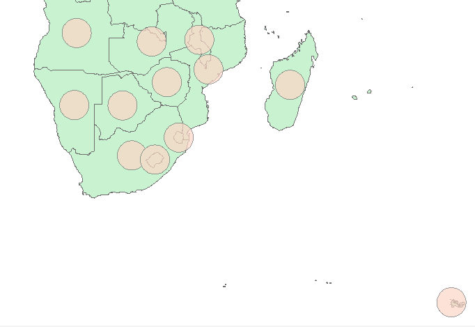
Centroid() and Buffer() are just two examples of the many availabe methods for producing a new geometry in GDAL. In this lesson's homework assignment, you will instead have to use the ogr.CreateGeometryFromWkt(...) function that we used earlier in this section to create a clip polygon from a WKT string representation but, apart from that, the order of operations for creating the output feature will be the same. The GDAL/OGR cookbook [48] contains many Python examples for working with vector data with GDAL, including how to create different kinds of geometries [49] from different input formats, calculating envelopes, lengths and areas of a geometry [50], and intersecting and combining geometries [51]. We recommend that you take a bit of time to browse through these online examples to get a better idea of what is possible. Then we move on to have a look at raster manipulation with GDAL.
3.9.2 Working with raster data
To open an existing raster file in GDAL, you would use the Open(...) function defined in the gdal module. The raster file we will use in the following examples contains world-wide bioclimatic data and will be used again in the lesson’s walkthrough. Download the raster file here [52].
raster = gdal.Open(r'c:\489\L3\wc2.0_bio_10m_01.tif')
We now have a GDAL raster dataset in variable raster. Raster datasets are organized into bands. The following command shows that our raster only has a single band:
raster.RasterCount
Output:
1
To access one of the bands, we can use the GetRasterBand(...) method of a raster dataset and provide the number of the band as a parameter (counting from 1, not from 0!):
band = raster.GetRasterBand(1) # get first band of the raster
If your raster has multiple bands and you want to perform the same operations for each band, you would typically use a for-loop to go through the bands:
for i in range(1, raster.RasterCount + 1):
    b = raster.GetRasterBand(i)
    print(b.GetMetadata())      # or do something else with b
There are a number of methods to read different properties of a band in addition to GetMetadata() used in the previous example, such as GetNoDataValue(), GetMinimum(), GetMaximum(), andGetScale().
print(band.GetNoDataValue())
print(band.GetMinimum())
print(band.GetMaximum())
print(band.GetScale())
Output:
-1.7e+308
-53.702073097229
33.260635217031
1.0
GDAL provides a number of operations that can be employed to create new files from bands. For instance, the gdal.Polygonize(...) function can be used to create a vector dataset from a raster band by forming polygons from adjacent cells that have the same value. To apply the function, we first create a new vector dataset and layer in it. Then we add a new field ‘DN’ to the layer for storing the raster values for each of the polygons created:
drv = ogr.GetDriverByName('ESRI Shapefile')
outfile = drv.CreateDataSource(r'c:\489\L3\polygonizedRaster.shp')
outlayer = outfile.CreateLayer('polygonized raster', srs = None )
newField = ogr.FieldDefn('DN', ogr.OFTReal)
outlayer.CreateField(newField)
Once the shapefile is prepared, we call Polygonize(...) and provide the band and the output layer as parameters plus a few additional parameters needed:
gdal.Polygonize(band, None, outlayer, 0, [])
outfile = None
With the None for the second parameter we say that we don’t want to provide a mask for the operation. The 0 for the fourth parameter is the index of the field to which the raster values shall be written, so the index of the newly added ‘DN’ field in this case. The last parameter allows for passing additional options to the function but we do not make use of this, so we provide an empty list. The second line "outfile = None" is for closing the new shapefile and making sure that all data has been written to it. The result produced in the new shapefile rasterPolygonized.shp should look similar to the image below when looked at in a GIS and using a classified symbology based on the values in the ‘DN’ field.

Polygonize(...) is an example of a GDAL function that operates on an individual band. GDAL also provides functions for manipulating raster files directly, such as gdal.Translate(...) for converting a raster file into a new raster file. Translate(...) is very powerful with many parameters and can be used to clip, resample, and rescale the raster as well as convert the raster into a different file format. You will see an example of Translate(...) being applied in the lesson’s walkthrough. gdal.Warp(...) is another powerful function that can be used for reprojecting and mosaicking raster files.
While the functions mentioned above and similar functions available in GDAL cover many of the standard manipulation and conversion operations commonly used with raster data, there are cases where one directly wants to work with the values in the raster, e.g. by applying raster algebra operations. The approach to do this with GDAL is to first read the data of a band into a GDAL multi-dimensional array object with the ReadAsArray() method, then manipulate the values in the array, and finally write the new values back to the band with the WriteArray() method.
data = band.ReadAsArray()
data
If you look at the output of this code, you will see that the array in variable data essentially contains the values of the raster cells organized into rows. We can now apply a simple mathematical expression to each of the cells, like this:
data = data * 0.1
data
The meaning of this expression is to create a new array by multiplying each cell value with 0.1. You should notice the change in the output from +308 to +307. The following expression can be used to change all values that are smaller than 0 to 0:
print(data.min())
data [ data < 0 ] = 0
print(data.min())
data.min() in the previous example is used to get the minimum value over all cells and show how this changes to 0 after executing the second line. Similarly to what you saw with pandas data frames in Section 3.8.6, an expression like data < 0 results in a Boolean array with True for only those cells for which the condition <0 is true. Then this Boolean array is used to select only specific cells from the array with data[...] and only these will be changed to 0. Now, to finally write the modified values back to a raster band, we can use the WriteArray(...) method. The following code shows how one can first create a copy of a raster with the same properties as the original raster file and then use the modified data to overwrite the band in this new copy:
drv = gdal.GetDriverByName('GTiff')     # create driver for writing geotiff file
outRaster = drv.CreateCopy(r'c:\489\newRaster.tif', raster , 0 )   # create new copy of inut raster on disk
newBand = outRaster.GetRasterBand(1)                               # get the first (and only) band of the new copy
newBand.WriteArray(data)                                           # write array data to this band
outRaster = None                                                   # write all changes to disk and close file
This approach will not change the original raster file on disk. Instead of writing the updated array to a band of a new file on disk, we can also work with an in-memory copy instead, e.g. to then use this modified band in other GDAL operations such as Polygonize(...) . An example of this approach will be shown in the walkthrough of this lesson. Here is how you would create the in-memory copy combining the driver creation and raster copying into a single line:
tmpRaster = gdal.GetDriverByName('MEM').CreateCopy('', raster, 0) # create in-memory copy
The approach of using raster algebra operations shown above can be used to perform many operations such as reclassification and normalization of a raster. More complex operations like neighborhood/zonal based operators can be implemented by looping through the array and adapting cell values based on the values of adjacent cells. In the lesson’s walkthrough you will get to see an example of how a simple reclassification can be realized using expressions similar to what you saw in this section.
While the GDAL Python package allows for realizing the most common vector and raster operations, it is probably fair to say that it is not the most easy-to-use software API. While the GDAL Python cookbook [53] contains many application examples, it can sometimes take a lot of search on the web to figure out some of the details of how to apply a method or function correctly. Of course, GDAL has the main advantage of being completely free, available for pretty much all main operating systems and programming languages, and not tied to any other GIS or web platform. In contrast, the Esri ArcGIS API for Python discussed in the next section may be more modern, directly developed specifically for Python, and have more to offer in terms of visualization and high-level geoprocessing and analysis functions, but it is tied to Esri’s web platforms and some of the features require an organizational account to be used. These are aspects that need to be considered when making a choice on which API to use for a particular project. In addition, the functionality provided by both APIs only overlaps partially and, as a result, there are also merits in combining the APIs as we will do later on in the lesson’s walkthrough.
3.10 Esri ArcGIS API for Python
Esri’s ArcGIS API for Python was announced in summer 2016 and was officially released at the end of the same year. The goal of the API as stated in this ArcGIS blog [54] accompanying the initial release is to provide a pythonic GIS API that is powerful, modern, and easy to use. Pythonic here means that it complies with Python best practices regarding design and implementation and is embedded into the Python ecosystem leveraging standard classes and packages (pandas and numpy, for instance). Furthermore, the API is supposed to be “not tied to specific ArcGIS jargon and implementation patterns” (Singh, 2016) and has been developed specifically to work well with Jupyter Notebook. Most of the examples from the API’s website [14] actually come in the form of Jupyter notebooks.
The current version (at the time of this writing) is version 2.1.0.3 published in March 2023. The API consists of several modules for:
- managing a GIS hosted on ArcGIS Online or ArcGIS Enterprise/Portal (module arcgis.gis)
- administering environment settings (module arcgis.env)
- working with features and feature layers (module arcgis.features)
- working with raster data (module arcgis.raster)
- performing network analyses (module arcgis.network)
- distributed analysis of large datasets (module arcgis.Geoanalytics)
- performing geocoding tasks (module arcgis.geocoding)
- answering questions about locations (module arcgis.geoenrichment)
- manipulating geometries (module arcgis.geometry)
- creating and sharing geoprocessing tools (module arcgis.geoprocessing)
- creating map presentations and visualizing data (module arcgis.mapping)
- processing real-time data feeds and streams (module arcgis.realtime)
- working with simplified representations of networks called schematics (module arcgis.schematics)
- embedding maps and visualizations as widgets, for instance within a Jupyter Notebook (module arcgis.widgets)
You will see some of these modules in action in the examples provided in the rest of this section.
Singh, R. (2016). ArcGIS Python API 1.0 Released. ArcGIS Blog. retrieved March 23, 2018 from https://blogs.esri.com/esri/arcgis/2016/12/19/arcgis-python-api-1-0-released/
3.10.1 GIS, map and content
The central class of the API is the GIS class defined in the arcgis.gis module. It represents the GIS you are working with to access and publish content or to perform different kinds of management or analysis tasks. A GIS object can be connected to AGOL or Enterprise/Portal for ArcGIS. Typically, the first step of working with the API in a Python script consists of constructing a GIS object by invoking the GIS(...) function defined in the argis.gis module. There are many different ways of how this function can be called, depending on the target GIS and the authentication mechanism that should be employed. Below we are showing a couple of common ways to create a GIS object before settling on the approach that we will use in this class, which is tailored to work with your pennstate organizational account.
Most commonly, the GIS(...) function is called with three parameters, the URL of the ESRI web GIS to use (e.g. ‘https://www.arcgis.com’ for a GIS object that is connected to AGOL), a username, and the login password of that user. If no URL is provided, the default is ArcGIS Online and it is possible to create a GIS object anonymously without providing username and password. So the simplest case would be to use the following code to create an anonymous GIS object connected to AGOL (we do not recommend running this code - it is shown only as an example):
from arcgis.gis import GIS
gis = GIS()
Due to not being connected to a particular user account, the available functionality will be limited. For instance, you won’t be able to upload and publish new content. If, instead, you'd want to create the GIS object but with a username and password for a normal AGOL account (so not an enterprise account), you would use the following way with <your username> and <your password> replaced by the actual user name and password (we do not recommend running this code either- it is shown only as an example):
from arcgis.gis import GIS
gis = GIS('https://www.arcgis.com', '<your username>', '<your password>')
gis?
This approach unfortunately does not work with the pennstate organizational account you had to create at the beginning of the class. But we will need to use this account in this lesson to make sure you have the required permissions. You already saw how to connect with your pennstate organizational account if you tried out the test code in Section 3.2. The URL needs to be changed to ‘https://pennstate.maps.arcgis.com’ and we have to use a parameter called client_id to provide the ID of an app that we created for this class on AGOL. When using this approach, calling the GIS(...) function will open a browser window where you can authenticate with your PSU credentials and/or you will be asked to grant the permission to use Python with your pennstate AGOL account. After that, you will be given a code that you have to paste into a box that will be showing up in your notebook. The details of what is going on behind the scenes are a bit complicated but whenever you need to create a GIS object in this class to work with the API, you can simply use these exact few lines and then follow the steps we just described. The last line of the code below is for testing that the GIS object has been created correctly. It will print out some help text about the GIS object in a window at the bottom of the notebook. The screenshot below illustrates the steps needed to create the GIS object and the output of the gis? command. (for safety it would be best to restart your Notebook kernel prior to running the code below if you did run the code above as it can cause issues with the below instructions working properly)
import arcgis
from arcgis.gis import GIS
gis = GIS('https://pennstate.maps.arcgis.com', client_id='lDSJ3yfux2gkFBYc')
gis?
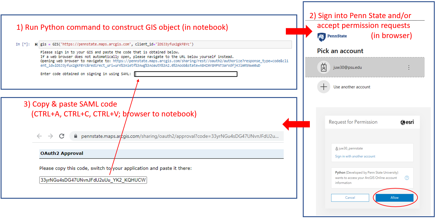
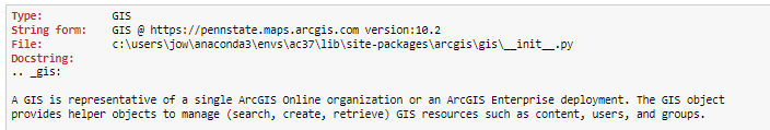
The GIS object in variable gis gives you access to a user manager (gis.users), a group manager (gis.groups) and a content manager (gis.content) object. The first two are useful for performing administrative tasks related to groups and user management. If you are interested in these topics, please check out the examples on the Accessing and Managing Users [55] and Batch Creation of Groups [56] pages. Here we simply use the get(...) method of the user manager to access information about a user, namely ourselves. Again, you will have to replace the <your username> tag with your PSU AGOL name to get some information display related to your account:
user = gis.users.get('<your username>')
user
The user object now stored in variable user contains much more information about the given user in addition to what is displayed as the output of the previous command. To see a list of available attributes, type in
user.
and then press the TAB key for the Jupyter autocompletion functionality. The following command prints out the email address associated with your account:
user.email
We will talk about the content manager object in a moment. But before that, let’s talk about maps and how easy it is to create a web map like visualization in a Jupyter Notebook with the ArcGIS API. A map can be created by calling the map(...) method of the GIS object. We can pass a string parameter to the method with the name of a place that should be shown on the map. The API will automatically try to geocode that name and then set up the parameters of the map to show the area around that place. Let’s use State College as an example:
map = gis.map('State College, PA')
map
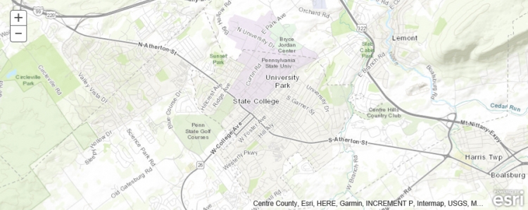
The API contains a widget for maps so that these will appear as an interactive map in a Jupyter Notebook. As a result, you will be able to pan around and use the buttons at the top left to zoom the map. The map object has many properties and methods that can be used to access its parameters, affect the map display, provide additional interactivity, etc. For instance, the following command changes the zoom property to include a bit more area around State College. The map widget will automatically update accordingly.
map.zoom = 11
With the following command, we change the basemap tiles of our map to satellite imagery. Again the map widget automatically updates to reflect this change.
map.basemap = 'satellite'
As another example, let’s add two simple circle marker objects to the map, one for Walker Building on the PSU campus, the home of the Geography Department, and one for the Old Main building. The ArcGIS API provides a very handy geocode(...) function in the arcgis.geocoding module so that we won’t have to type in the coordinates of these buildings ourselves. The properties of the marker are defined in the pt_sym dictionary.
from arcgis.geocoding import geocode

pt_sym = {
    "type": "esriSMS",
    "style": "esriSMSCircle",
    "color": [255,0,0,255],
}

walker = geocode('Walker Bldg, State College, PA')[0]
oldMain = geocode('Old Main Bldg, State College, PA')[0]
map.draw(walker, {'title':'Walker Bldg', 'content': walker['attributes']['LongLabel']}, symbol=pt_sym)
map.draw(oldMain, {'title':'Old Main Bldg', 'content': oldMain['attributes']['LongLabel']}, symbol=pt_sym)
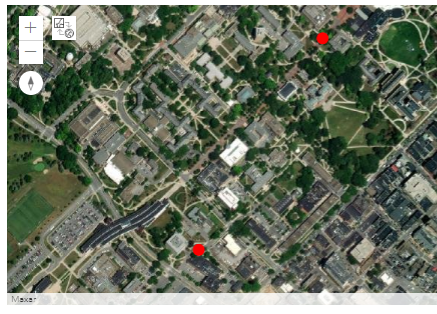
The map widget should now include the markers for the two buildings as shown in the image above (the markers may look different). A little explanation on what happens in the code: the geocode(...) function returns a list of candidate entities matching the given place name or address, with the candidate considered most likely appearing as the first one in the list. We here simply trust that the ArcGIS API has been able to determine the correct candidate and hence just take the first object from the respective lists via the “[0]” in the code. What we have now stored in variables walker and oldMain are dictionaries with many attributes to describe the entities. When adding the markers to the map, we provide the respective variables as the first parameter and the API will automatically access the location information in the dictionaries to figure out where the marker should be placed. The second parameter is a dictionary that specifies what should be shown in the popup that appears when you click on the marker. We use short names for the title of the popups and then use the ‘LongLabel’ property from the dictionaries, which contains the full address, for the content of the popups.
Let's have a look at a last map example demonstrating how one can use the API to manually draw a route from Walker building to Old Main and have the API calculate the length of that route. The first thing we do is import the lengths(...) function from the arcgis.geometry module and define a function that will be called once the route has been drawn to calculate the length of the resulting polyline object that is passed to the function in parameter g:
from arcgis.geometry import lengths

def calcLength(map,g):
    length = lengths(g['spatialReference'], [g], "", "geodesic")
    print('Length: '+ str(length[0]) + 'm.')
Once the length has been computed, the function will print out the result in meters. We now register this function as the function to be called when a drawing action on the map has terminated. In addition, we define the symbology for the drawing to be a dotted red line:
map.on_draw_end(calcLength)

line_sym = {
"type": "esriSLS",
"style": "esriSLSDot",
"color": [255,0,0,255],
"width": 3
}
With the next command we start the drawing with the ‘polyline’ tool. Before you execute the command, it's a good idea to make sure the map widget is zoomed in to show the area between the two markers but you will still be able to pan the map by dragging with the left mouse button pressed and to zoom with the mouse wheel during the drawing. You need to do short clicks with the left mouse button to set the points for the start point and end points of the line segments. To end the polyline, make a double click for the last point while making sure you don't move the mouse at the same time. After this, the calculated distance will appear under the map widget.
map.draw('polyline', symbol=line_sym)
You can always restart the drawing by executing the previous code line again. Using the command map.clear_graphics() allows for clearing all drawings from the map but you will have to recreate the markers after doing so.
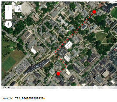
Now let’s get back to the content manager object of our GIS. The content manager object allows us to search and use all the content we have access to. That includes content we have uploaded and published ourselves but also content published within our organization and content that is completely public on AGOL. Content can be searched with the search(...) method of the content manager object. The method takes a query string as parameter and has additional parameters for setting the item type we are looking for and the maximum number of entries returned as a result for the query. For instance, try out the following command to get a list of available feature services that have PA in the title:
featureServicesPA = gis.content.search(query='title:PA', item_type='Feature Layer Collection', max_items = 50)
featureServicesPA
This will display a list of different AGOL feature service items available to you. The list is probably rather short at the moment because not much has been published in the new pennstate organization yet, but there should at least be one entry with municipality polygons for PA. Each feature service from the returned list can, for instance, be added to your map or used for some spatial analysis. To add a feature service to your map as a new layer, you have to use the add_layer(...) method of the map object. For example, the following command takes the first feature service from our result list in variable featureServicesPA and adds it to our map widget:
map.add_layer(featureServicesPA[0], {'opacity': 0.8})
The first parameter specifies what should be added as a layer (the feature service with index 0 from our list in this case), while the second parameter is an optional dictionary with additional attributes (e.g., opacity, title, visibility, symbol, renderer) specifying how the layer should be symbolized and rendered. Feel free to try out a few other queries (e.g. using "*" for the query parameter to get a list of all available feature services) and adding a few other layers to the map by changing the index used in the previous command. If the map should get too cluttered, you can simply recreate the map widget with the map = gis.map(...) command from above.
The query string given to search(...) can contain other search criteria in addition to ‘title’. For instance, the following command lists all feature services that you are the owner of (replace <your agol username> with your actual Penn State AGOL/Pro user name):
gis.content.search(query='owner:<your agol username>', item_type='Feature Service')
Unless you have published feature services in your AGOL account, the list returned by this search will most likely be empty ([]). So how can we add new content to our GIS and publish it as a feature service? That’s what the add(...) method of the content manager object and the publish(...) method of content items are for. The following code uploads and publishes a shapefile of larger cities in the northeast of the United States.
To run it, you will need to first download the zipped shapefile [57] and then slightly change the filename on your computer. Since AGOL organizations must have unique services names, edit the file name to something like ne_cities_[initials].zip or ne_cities_[your psu id].zip so the service name will be unique to the organization. Adapt the path used in the code below to refer to this .zip file on your disk.
neCities = gis.content.add({'type': 'Shapefile'}, r'C:\489\L3\ne_cities.zip')
neCitiesFS = neCities.publish()
The first parameter given to gis.content.add(...) is a dictionary that can be used to define properties of the data set that is being added, for instance tags, what type the data set is, etc. Variable neCitiesFS now refers to a published content item of type arcgis.gis.Item that we can add to a map with add_layer(...). There is a very slight chance that this layer will not load in the map. If this happens for you - continue and you should be able to do the buffer & intersection operations later in the walkthrough without issue. Let’s do this for a new map widget:
cityMap = gis.map('Pennsylvania')
cityMap.add_layer(neCitiesFS, {})
cityMap
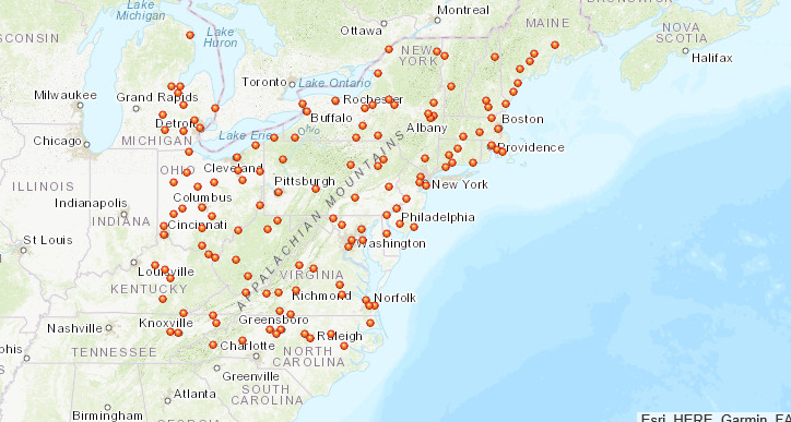
The image shows the new map widget that will now be visible in the notebook. If we rerun the query from above again...
gis.content.search(query='owner:<your agol username>', item_type='Feature Service')
...our newly published feature service should now show up in the result list as:
<Item title:"ne_cities" type:Feature Layer Collection owner:<your AGOL username>>
3.10.2 Accessing features and geoprocessing tools
The ArcGIS Python API also provides the functionality to access individual features in a feature layer, to manipulate layers, and to run analyses from a large collection of GIS tools including typical GIS geoprocessing tools. Most of this functionality is available in the different submodules of arcgis.features. To give you a few examples, let’s continue with the city feature service we still have in variable neCitiesFS from the previous section. A feature service can actually have several layers but, in this case, it only contains one layer with the point features for the cities. The following code example accesses this layer (neCitiesFE.layers[0]) and prints out the names of the attribute fields of the layer by looping through the ...properties.fields list of the layer:
for f in neCitiesFS.layers[0].properties.fields:
	print(f)
When you try this out, you should get a list of dictionaries, each describing a field of the layer in detail including name, type, and other information. For instance, this is the description of the STATEABB field:
{
 "name": "STATEABB",
 "type": "esriFieldTypeString",
 "actualType": "nvarchar",
 "alias": "STATEABB",
 "sqlType": "sqlTypeNVarchar",
 "length": 10,
 "nullable": true,
 "editable": true,
 "domain": null,
 "defaultValue": null
 }
The query(...) method allows us to create a subset of the features in a layer using an SQL query string similar to what we use for selection by attribute in ArcGIS itself or with arcpy. The result is a feature set in ESRI terms. If you look at the output of the following command, you will see that this class stores a JSON representation of the features in the result set. Let’s use query(...) to create a feature set of all the cities that are located in Pennsylvania using the query string "STATEABB"='US-PA' for the where parameter of query(...):
paCities = neCitiesFS.layers[0].query(where='"STATEABB"=\'US-PA\'')
print(paCities.features)
paCities
Output:
[{"geometry": {"x": -8425181.625237303, "y": 5075313.651659228},
"attributes": {"FID": 50, "OBJECTID": "149", "UIDENT": 87507, "POPCLASS": 2, "NAME":
"Scranton", "CAPITAL": -1, "STATEABB": "US-PA", "COUNTRY": "USA"}}, {"geometry":
{"x": -8912583.489066456, "y": 5176670.443556941}, "attributes": {"FID": 53,
"OBJECTID": "156", "UIDENT": 88707, "POPCLASS": 3, "NAME": "Erie", "CAPITAL": -1,
"STATEABB": "US-PA", "COUNTRY": "USA"}}, ...  ]
<FeatureSet> 10 features
Of course, the queries we can use with the query(...) function can be much more complex and logically connect different conditions. The attributes of the features in our result set are stored in a dictionary called attributes for each of the features. The following loop goes through the features in our result set and prints out their name (f.attributes['NAME']) and state (f.attributes['STATEABB']) to verify that we only have cities for Pennsylvania now:
for f in paCities:
	print(f.attributes['NAME'] + " - "+ f.attributes['STATEABB'])
Output:
Scranton - US-PA
Erie - US-PA
Wilkes-Barre - US-PA
...
Pittsburgh - US-PA
Now, to briefly illustrate some of the geoprocessing functions in the ArcGIS Python API, let’s look at the example of how one would determine the parts of the Appalachian Trail that are within 30 miles of a larger Pennsylvanian city. For this we first need to upload and publish another data set, namely one that’s representing the Appalachian Trail. We use a data set that we acquired from PASDA [58] for this, and you can download the DCNR_apptrail file here [59]. As with the cities layer earlier, there is a very small chance that this will not display for you - but you should be able to continue to perform the buffer and intersection operations. The following code uploads the file to AGOL (don’t forget to adapt the path and add your initials or ID to the name!), publishes it, and adds the resulting trail feature service to your cityMap from above:
appTrail = gis.content.add({'type': 'Shapefile'}, r'C:\489\L3\dcnr_apptrail_2003.zip')
appTrailFS = appTrail.publish()
cityMap.add_layer(appTrailFS, {})
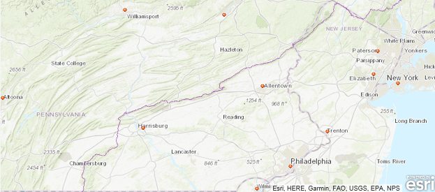
Next, we create a 30 miles buffer around the cities in variable paCities that we can then intersect with the Appalachian Trail layer. The create_buffers(...) function that we will use for this is defined in the arcgis.features.use_proximity module together with other proximity based analysis functions. We provide the feature set we want to buffer as the first parameter, but, since the function cannot be applied to a feature set directly, we have to invoke the to_dict() method of the feature set first. The second parameter is a list of buffer distances allowing for creating multiple buffers at different distances. We only use one distance value, namely 30, here and also specify that the unit is supposed to be ‘Miles’. Finally, we add the resulting buffer feature set to the cityMap above.
from arcgis.features.use_proximity import create_buffers
bufferedCities = create_buffers(paCities.to_dict(), [30], units='Miles')
cityMap.add_layer(bufferedCities, {})
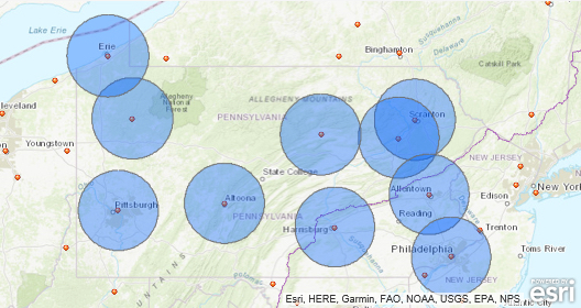
As the last step, we use the overlay_layers(...) function defined in the arcgis.features.manage_data module to create a new feature set by intersecting the buffers with the Appalachian Trail polylines. For this we have to provide the two input sets as parameters and specify that the overlay operation should be ‘Intersect’.
from arcgis.features.manage_data import overlay_layers
trailPartsCloseToCity = overlay_layers(appTrailFS, bufferedCities, overlay_type='Intersect')
We show the result by creating a new map ...
resultMap = gis.map('Pennsylvania')
resultMap
... and just add the features from the resulting trailPartsCloseToCity feature set to this map:
resultMap.add_layer(trailPartsCloseToCity)
The result is shown in the figure below.
3.10.3 More examples and additional materials
This section gave you a brief introduction to ESRI's ArcGIS API for Python and showed you some of the most important methods and patterns that you will typically encounter when using the API. The API is much too rich to cover everything here, so, to get a better idea of the geoprocessing and other capabilities of the API, we recommend that you check and try out some of the sample notebooks [60] that ESRI has published, such as:
- Chennai Floods 2015 - a geographic analysis [61]
- Fighting California forest fires using spatial analysis [62]
A lot of valuable information can also be gained from the ESRI's API guide [63], and, of course, the API documentation [64].
3.11 Walkthrough: Species distribution modeling with Jupyter
You now have a basic understanding of the species distribution modeling task we want to solve in this lesson's walkthrough as well as the different Python packages that will play a role in preparing the data, running the model, and visualizing the result. Since all of this will take place within a Jupyter notebook, the remainder of this section will consist of the notebook itself exported to html and embedded into the Drupal pages for this lesson. Here is the link to the data you need for this walkthrough:
Link to L3 Walkthrough data, which you will need to download and extract to a new folder [65]
Instead of just reading through the HTML version of the notebook content linked below, you should download the notebook [66], extract the contained .ipynb notebook file, place it in your user home or documents folder, open it with Jupyter and work through it step-by-step following the instructions given in the notebook itself, executing the code cells, and trying to understand the code sections and the output they produce.
Important note: Sections 3.1 and 5.2 of the notebook will use the Python-to-R interface (Section 3.7 of the lesson materials). On the R side, there are three packages involved: dismo, maptools, and rgdal.
While the environment we installed in Section 3.2 contains conda packages for dismo and maptools, there is at the moment no conda package available for rgdal because of technical issues the package maintainers have to resolve (see https://github.com/conda-forge/r-rgdal-feedstock/issues/18 [67]). We are therefore currently installing the rgdal package in the notebook code itself with the line "%R install.packages('rgdal')" close to the beginning. However, we in the past had a very few cases where this caused problems on some computers. Just in case you find yourself unable to run some of the R commands (starting with %R) in sections 3.1 and 5.2 of the notebook, we are here providing two files [68] that can be used as a workaround. You will then have to place these files in your workspace folder for this walkthrough (just read the corresponding sections in the HTML export of the notebook linked below to see the output produced by the steps you cannot run yourself) and then follow the workaround instructions in the notebook that explain how to continue with the other sections with the help of these two files.
Here is the link to html export of the notebook if you want to have a look at it outside of Jupyter Notebook: HTML export of the walkthrough notebook [69]
Reminder:
Complete all of the lesson tasks!
You have finished the Lesson 3 course materials. On the next pages, you will find a few practice exercises and the instructions for the Lesson 3 homework assignment. Double-check the list of requirements on the Lesson 3 Checklist page to make sure you have completed all of the activities listed there before beginning the next lesson.
3.12 Lesson 3 Practice Exercises
Again, we are going to close out the lesson with a few practice exercises that focus on the new Python concepts introduced in this lesson (regular expressions and higher order functions) as well as on working with tabular data with pandas as a preparation for this lesson's homework assignment. In the homework assignment, you are also going to use geopandas, the Esri ArcGIS for Python API, and GDAL/OGR again to get some more practice with these libraries, too. What was said in the introduction to the practice exercises of Lesson 2 holds here as well: don't worry if you have troubles finding the perfect solution on your own. Studying the solutions carefully is another way of learning and improving your skills. The solutions of the three practice exercises pages can again be found in the following subsections.
Practice Exercise 1: Regular Expressions (see Section 3.3)
Write a function that tests whether an entered string is a valid date using the format "YYYY-MM-DD". The function takes the string to test as a parameter and then returns True or False. The YYYY can be any 4-digit number, but the MM needs to be a valid 2-digit number for a month (with a leading 0 for January to September). The DD needs to be a number between 01 and 31 but you don’t have to check whether this is a valid number for the given month. Your function should use a single regular expression to solve this task.
Here are a few examples you can test your implementation with:
"1977-01-01"  -> True

"1977-00-01"  -> False (00 not a valid month)

"1977-23-01"  -> False (23 not a valid month)

"1977-12-31"  -> True

"1977-11-01asdf"  -> False (you need to make sure there are no additional characters after the date)

"asdf1977-11-01"  -> False (you need to make sure there are no additional characters before the date)

"9872-12-31"  -> True

"0000-12-33"  -> False (33 is not a valid day)

"0000-12-00"  -> False (00 not a valid day)

"9872-15-31"  -> False (15 is not a valid month)
Practice Exercise 2: Higher Order Functions (see Section 3.4)
We mentioned that the higher-order function reduce(...) can be used to do things like testing whether all elements in a list of Booleans are True. This exercise has three parts:
- Given list l containing only Boolean values as elements (e.g. l = [ True, False, True ]), use reduce(…) to test whether all elements in l are True? What would you need to change to test if at least one element is True? (Hint: you will have to figure out what the right logical operator to use is and then look at how it’s called in the Python module operator; then figure out what the right initial value for the third parameter of reduce(...) is.)
- Now instead of a list of Booleans, you have a list of integer numbers (e.g. l =[-4, 2, 1, -6 ]). Use a combination of map(…) and reduce(…) to check whether or not all numbers in the list are positive numbers (> 0).
- Implement reduce(...) yourself and test it with the example from part 1. Your function myReduce(…) should have the three parameters f (function), l (list), and i (initial value). It should consist of a for-loop that goes through the elements of the list and it is not allowed to use any other higher order function (in particular not the actual reduce(...) function).
Practice Exercise 3: Pandas (see Section 3.8)
Below is an imaginary list of students and scores for three different assignments.
| Name | Assignment 1 | Assignment 2 | Assignment 3 | |
|---|---|---|---|---|
| 1 | Mike | 7 | 10 | 5.5 |
| 2 | Lisa | 6.5 | 9 | 8 |
| 3 | George | 4 | 3 | 7 |
| 4 | Maria | 7 | 9.5 | 4 |
| 5 | Frank | 5 | 5 | 5 |
Create a pandas data frame for this data (e.g. in a fresh Jupyter notebook). The column and row labels should be as in the table above.
Now, use pandas operations to add a new column to that data frame and assign it the average score over all assignments for each row.
Next, perform the following subsetting operations using pandas filtering with Boolean indexing:
- Get all students with an Assignment 1 score < 7 (show all columns)
- Get all students with Assignment 1 and Assignment 2 scores both > 6 (show all columns)
- Get all students with at least one score < 5 over all assignments (show all columns)
(Hint: an alternative to using the logical or (|) over all columns with scores is to call the .min(…) method of a data frame with the parameter "axis = 1" to get the minimum value over all columns for each row. This can be used here to first create a vector with the minimum score over all three assignments and then create a Boolean vector from it based on whether or not the value is <5. You can then use this vector for the Boolean indexing operation.)
- Get all students whose names start with 'M' and only show the name and average score columns
(Hint: there is also a method called .map(…) that you can use to apply a function or lambda expression to a pandas data frame (or individual column). The result is a new data frame with the results of applying the function/expression to each cell in the data frame. This can be used here to create a Boolean vector based on whether or not the name starts with ‘M’ (string method startswith(…)). This vector can then be used for the Boolean indexing operation. Then you just have to select the columns of interest with the last part of the statement).
- Finally, sort the table by name.
Lesson 3 Exercise 1 Solution
import re

datePattern = re.compile('\d\d\d\d-(0[1-9]|1[0-2])-(0[1-9]|[12]\d|3[01])$')

def isValidDate(s):
    return datePattern.match(s) != None
Explanation: Since we are using match(…) to compare the compiled pattern in variable datePattern to the string in parameter s given to our function isValidDate(…), we don’t have to worry about additional characters before the start of the date because match(…) will always try to match the pattern to the start of the string. However, we use $ as the last character in our pattern to make sure there are no additional characters following the date. That means the pattern has the form
“…-…-…$”
where the dots have to be replaced with some regular expression notation for the year, month, and day parts. The year part is easy, since we allow for any 4-digit number here. So we can use \d\d\d\d here, or alternatively \d{4,4} (remember that \d stands for the predefined class of all digits).
For the month, we need to distinguish two cases: either it is a 0 followed by one of the digits 1-9 (but not another 0) or a 1 followed by one of the digits 0-2. We therefore write this part as a case distinction (…|…) with the left part 0[1-9] representing the first option and the second part 1[0-2] representing the second option.
For the day, we need to distinguish three cases: (1) a 0 followed by one of the digits 1-9, (2) a 1 or 2 followed by any digit, or (3) a 3 followed by a 0 or a 1. Therefore we use a case-distinction with three options (…|…|…) for this part. The first part 0[1-9] is for option (1), the second part [12]\d for option (2), and the third part 3[01] for the third option.
Lesson 3 Exercise 2 Solution
Part 1:
import operator

from functools import reduce

l = [True, False, True]

r = reduce(operator.and_, l, True)

print(r)  #  output will be False in this case
To check whether or not at least one element is True, the call has to be changed to:
r = reduce(operator.or_, l, False)
Part 2:
import operator

from functools import reduce

l = [-4, 2, 1, -6 ]

r = reduce(operator.and_, map(lambda n: n > 0, l), True)

print(r)   # will print False in this case
We use map(…) with a lambda expression for checking whether or not an individual element from the list is >0. Then we apply the reduce(…) version from part 1 to the resulting list of Boolean values we get from map(…) to check whether or not all elements are True.
Part 3:
import operator

l = [True, False, True]

def myReduce(f, l, i):
	intermediateResult = i
	for element in l:
		intermediateResult = f(intermediateResult, element)
	return intermediateResult

r = myReduce(operator.and_, l, True)
print(r)  #  output will be False in this case
Maybe you were expecting that an implementation of reduce would be more complicated, but it’s actually quite simple. We set up a variable to always contain the intermediate result while working through the elements in the list and initialize it with the initial value provided in the third parameter i. When looping through the elements, we always apply the function given in parameter f to the intermediate result and the element itself and update the intermediate result variable with the result of this operation. At the end, we return the value of this variable as the result of the entire reduce operation.
Lesson 3 Exercise 3 Solution
import pandas as pd

# create the data frame from a list of tuples
data = pd.DataFrame( [('Mike',7,10,5.5),
     ('Lisa', 6.5, 9, 8),
     ('George', 4, 3, 7),
     ('Maria', 7, 9.5, 4),
     ('Frank', 5, 5, 5) ] )

# set column names
data.columns = ['Name', 'Assignment 1', 'Assignment 2', 'Assignment 3']

# set row names
data.index = range(1,len(data)+1)

# show table
print(data)

# add column with averages
data['Average'] = (data['Assignment 1'] + data['Assignment 2'] + data['Assignment 3']) / 3

# part a (all students with a1 score < 7)
print(data[ data['Assignment 1'] < 7])

# part b (all students with a1 and a2 score > 6)
print(data[ (data['Assignment 1'] > 6) & (data['Assignment 2'] > 6)])

# part c (at least one assignment < 5)
print( data[ data[ ['Assignment 1', 'Assignment 2', 'Assignment 3'] ].min(axis = 1) < 5 ] )

# part d (name starts with M, only Name and Average columns)
print(data [ data [ 'Name' ].map(lambda x: x.startswith('M')) ] [ ['Name','Average'] ])

# sort by Name
print(data.sort_values(by = ['Name']))
If any of these steps is unclear to you, please ask for further explanation on the forums.
3.13 Lesson 3 Assignment
In this homework assignment, we want you to practice working with pandas and the other Python packages introduced in this lesson some more, and you are supposed to submit your solution as a nice-looking Jupyter Notebook including well-formatted explanations of each step. While the assignment could be solved using pandas, geopandas, and the Esri Python API alone, we are asking you to use GDAL/OGR for one of the steps involved so that you get some further practice with that library as well. To solve the task, you will occasionally have to use the packages in ways that we did not show in the lesson materials. In addition, you will have to work with the Python datetime module for representing dates & times in Python code. That means you will also have to practice working with the respective documentations and complementing web resources a bit. However, we did include some pointers in the instructions below, so that you have an idea of where to look, and also provided some examples.
The situation is the following: You have been hired by a company active in the northeast of the United States to analyze and produce different forms of summaries for the traveling activities of their traveling salespersons. Unfortunately, the way the company has been keeping track of the related information leaves a lot to be desired. The information is spread out over numerous .csv files. Please download the .zip file containing all (imaginary) data [70] you need for this assignment and extract it to a new folder. Then open the files in a text editor and read the explanations below.
Explanation of the files:
File employees.csv: Most data files of the company do not use the names of their salespersons directly but instead refer to them through an employee ID. This file maps employee name to employee ID number. It has two columns, the first contains the full names in the format first name, last name and the second contains the ID number. The double quotes around the names are needed in the csv file to signal that this is the content of a single cell containing a comma rather than two cells separated by a comma.
"Smith, Richard",1234421
"Moore, Lisa",1231233
"Jones, Frank",2132222
"Brown, Justine",2132225
"Samulson, Roger",3981232
"Madison, Margaret",1876541
Files travel_???.csv: each of these files describes a single trip by a salesperson. The number in the file name is not the employee ID but a trip number. There are 75 such files with numbers from 1001 to 1075. Each file contains just a single row; here is the content of one of the files, the one named travel_1001.csv:
2132222,2016-01-07 16:00:00,2016-01-26 12:00:00,Cleveland;Bangor;Erie;Philadelphia;New York;Albany;Cleveland;Syracuse
The four columns (separated by comma) have the following content:
- the ID of the employee who did this trip (here: 2132222),
- the start date and time of the trip (here: 2016-01-07 16:00:00),
- the end date and time of the trip (here: 2016-01-26 12:00:00),
- and the route consisting of the names of the cities visited on the trip as a string separated by semi-colons (here: Cleveland;Bangor;Erie;Philadelphia;New York;Albany;Cleveland;Syracuse). Please note that the entire list of cities visited is just a single column in the csv file!
File ne_cities.shp: You already know this shapefile from the lesson content. It contains larger cities in the northeast U.S.A. as WGS84 points. The only attribute relevant for this exercise in addition to the point geometry is the NAME field containing the city names.
There are a few more files in the folder. They are actually empty but you are not allowed to delete these from the folder. This is to make sure that you have to be as specific as possible when using regular expressions for file names in your solution.
Your Task
The Python code you are supposed to write should take three things as input:
- a list of employee names (e.g., ['Jones, Frank', 'Brown, Justine', 'Samulson, Roger'] ),
- a start date (e.g., '2016-06-26'),
- and an end date as input (e.g., '2017-05-11').
It should then produce two output files:
- A new .csv file that lists the trips made by employees from the given employee name list that took place between the given start and end dates with all information from the respective travel_???.csv files as well as the name of the employee and the duration of each trip in days. The rows should be ordered by employee name -> trip duration -> start date -> end date. The figure below shows the exemplary content of this output file.
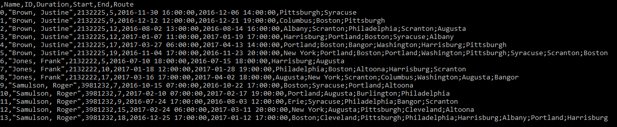 Example CSV Output File
 - A WGS1984 shapefile that shows the individual trips from the csv file created in (1) as polyline features. The attributes of the shapefile should be the name of the employee, the city list as a single string attribute, and the duration only. You will also have to zip this shapefile and upload & publish it as a feature service on ArcGIS Online.
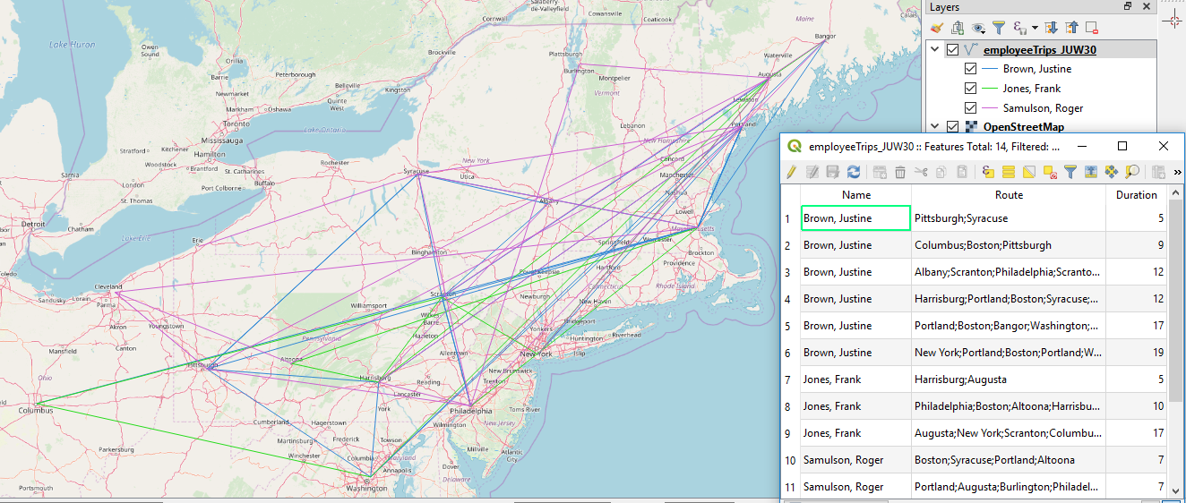 Example Output Shapefile Shown in QGIS
You should develop your solution as a Jupyter notebook with nicely formatted explanations of each step in your solution, similar to the L3 walkthrough notebook. Your notebook should at the end contain a map widget from the Esri Python API that displays the polyline feature service as a layer (similar to the lesson walkthrough notebook). You will submit this notebook file together with your write-up to the L3 assignment drop box on Canvas. The two images above have been produced using the example input values we gave above, so the name list 'Jones, Frank', 'Brown, Justine', and 'Samulson, Roger', the start date 2016-06-26, and the end date 2017-05-11. You can use this example for testing your solution.
Preparation
The assignment will require you to work with objects of the classes datetime and timedelta defined in the module datetime of the Python standard library to represent time stamps (combinations of date & time) and differences between them. The official documentation for the module is available at this Python documentation page [71]. In addition, you can find two links to introductions to datetime below that may be a bit easier to digest. Please check these out and make sure you understand how to work with the datetime class, how to compare datetime objects to see whether one is earlier than the other and how to calculate a timedelta object for the difference between two datetime objects. Time zones won’t matter in this assignment.
- Python DateTime, TimeDelta, Strftime (Format) with Examples [72]
- Working with datetime objects and timezones in Python [73]
Below are a few examples illustrating how to create datetime objects representing concrete dates, how to calculate the time difference (datetime object timedelta) between two datetime objects, and how to compare two datetime objects using the < or > operators. These examples should be easy to understand, in particular when you have read through the documentation linked above. If you have any remaining questions on using datetime, please ask them on the course forums.
import datetime

# create datetime objects for specific dates
date1 = datetime.datetime(2019, 1, 31, 17, 55)  # create datetime object for January 31, 2019, 17:55pm
date2 = datetime.datetime(2019, 3, 12, 0, 0)    # create datetime object for March 12, 2019, 0am
print(date1)
print(type(date1))
print(date2)
Output:
2019-01-31 17:55:00
<class 'datetime.datetime'>
2019-03-12 00:00:00
# calculate the time difference between two datetime objects
delta = date2 - date1
print(delta)
print(type(delta))
print(delta.days)     # difference in days
print(delta.seconds)  # difference in seconds
Output:
39 days, 6:05:00
<class 'datetime.timedelta'>
39
21900
# comparing datetime objects
if (date2 < date1):
    print('before')
else:
    print('after')
Output:
after
Steps in Detail:
Your notebook should roughly follow the steps below; in particular you should use the APIs mentioned for performing each of the steps:
- The input variables defined at the beginning of your notebook should include
- the list of employee names to include in the output
- the start date and end dates as datetime.datetime objects
- the folder that contains the input files
- the name of the output shapefile (include your initials or ID in the name to make the name unique for uploading it to AGOL)
- the name of the output csv file
- Use pandas (Section 3.8) to read the data from employees.csv into a data frame (see Hint 1).
- Use pandas to create a single data frame with the content from all 75 travel_???.csv files. The content from each file should form a row in the new data frame. The dates should be represented as datetime objects in the data frame (see Hints 1 and 2). Use regular expression and the functions from the re package for this step (Section 3.3) to only include files that start with "travel_", followed by a number, and ending in ".csv".
- Use pandas operations to join (see Section 3.8.5) the two data frames from steps (2) and (3) using the employee ID as key. Derive from this combined data frame a new data frame with
- only those rows that contain trips of employees from the input name list and with a start date after the given start date and an end date before the given end date (see Hint 3)
- an additional column that contains the duration of the trips in days (computed by subtracting start from end date)
- columns appearing in the order “Name”, “ID”, “Duration”, “Start”, “End”, and “Route” with these labels, and row labels being integer numbers 0,1,2,… (see image of example csv output file above)
- rows sorted by employees' names as the first criterion, followed by duration (meaning all trips for the same person are ordered from shortest to longest), start date, and end date as criteria.
- Write the data frame produced in the previous step to a new csv file using the specified output file name from (1) (see Hint 1 and image of example csv output file above).
- Use geopandas (Section 6.1 of the Juypter notebook from the lesson walkthrough) and its read_file(...) function to read the ne_cities.shp shapefile into a data frame. Reading a shapefile with the read_file(...) geopandas function is straightforward and you shouldn’t have any trouble finding some examples on the web. The result is a special geopandas data frame object that has a column called geometry which contains Shapely Point objects with WGS84 coordinates for the cities.
- Use GDAL/OGR (Section 3.9) to create a new shapefile with polyline features for each trip in the combined data frame from step (5) and attributes “Name” with the employee's name, “Route” with the city list for that trip, and “Duration” in days (see image of example output shapefile above). The polyline features need to be created from the city lists in the Route column and the point coordinates available in the geometry column of the ne_cities geopandas data frame produced in the previous step.
To create the new shapefile and populate it with features you can follow the general steps from creating the centroid buffer file in the last part of Section 3.9.1. The most tricky part will be to translate each trip into a WKT LineString that you then can create an OGR polyline feature from using the ogr.CreateGeometryFromWkt(...) function replacing the centroid and buffering part in the example from 3.9.1. Hint 4 shows how all the WKT LineStrings can be created to then be added as a new column to the combined data frame from step (5). This is done all in a single line with nested list comprehensions. If you feel very confident in your Python skills, you can try to write this code yourself (it doesn't necessarily have to be just a single line of code), else we recommend that you just use the code provided in the hint to do the translation. - Zip the shapefile produced in the previous step, then upload and publish it as a feature service on ArcGIS Online with the Esri API and include a map widget in your notebook showing the feature service as a layer (see Section 3.10 and the lesson walkthrough). You are allowed to reuse the code from the lesson walkthrough for this including the zipfile(...) function. Make sure that the name of the uploaded file is unique by incorporating your initials or ID).
Hint 1:
Pandas provides functions for reading and writing csv files (and quite a few other file formats). They are called read_csv(...) and to_csv(...). See this Pandas documentation site for more information [74] and also the Python datetime documentation [71]for datetime parsing specifics. When your input file contains dates that you want to become datetime objects, you should use the parse_dates and date_parser keyword arguments of read_csv(…) to let the method know which columns contain dates and how to interpret them (see the subsection on "Date Handling" on the page linked above). Here is an example of how this kind of command needs to look. The None for the header argument signals that the table in the csv file does not contain column names as the first row. The [...] for the parse_dates argument needs to be replaced by a list of column indices for the columns that contain dates in the csv file. The lambda function for the date_parser argument maps a date string we find in the input .csv file to a datetime object.
import pandas as pd
import datetime
df = pd.read_csv(r'C:\489\test.csv', sep=",", header=None, parse_dates=[...], date_parser= lambda x: datetime.datetime.strptime(x, '%Y-%m-%d %H:%M:%S'))
Hint 2:
The pandas concat(…) [75] function can be used to combine several data frames with the same columns stored in a list to form a single data frame. This can be a good approach for this step. Let's say you have the individual data frames stored in a list variable called dataframes. You'd then simply call concat like this:
combinedDataFrame = pd.concat(dataframes)
This means your main task will be to create the list of pandas data frames, one for each travel_???.csv file before calling concat(...). For this, you will first need to use a regular expression to filter the list of all files in the input folder you get from calling os.listdir(inputFolder) to only the travel_???.csv files and then use read_csv(...) as described under Hint 1 to create a pandas DataFrame object from the csv file and add this to the data frame list.
Hint 3:
You can compare a datetime object (e.g. the start or end date) to a datetime column in a pandas data frame resulting in a Boolean vector that tells you whether the comparison is true or not for each row. Furthermore, you can use the pandas method isin(…) [76] to check whether the string in the cells of a data frame or single column are contained in a given list of strings. The result is again a Boolean data frame/column. Together this allows you to select the desired rows via Boolean indexing as shown in Section 3.8.6. Here is a simple example showing how isin(...) is used to create a Boolean vector based on whether or not the name of each row is from a given list of names:
import pandas as pd
names = ['Frank', 'James', 'Jane', 'Stevie']    # names we are interested in
df = pd.DataFrame([['Martin', 5],               # simple data frame with two columns
                   ['James', 3],
                   ['Sue', 1],
                   ['Mark', 11],
                   ['Stevie',3 ]] , columns=['Name', 'Grade'])
booleanVector = df.Name.isin(names)
print(booleanVector)
Output:
0    False
1     True
2    False
3    False
4     True
Name: Name, dtype: bool
Hint 4:
The GDAL cookbook contains several examples of creating a polyline geometry from a WKT LineString that should be helpful to implement this step. In principle, the entire translation of the semi-colon-separated city list into a WKT LineString can be done with the following expression using two nested list comprehensions, but it is also ok if you break this down into several steps.
wkt = [ 'LineString (' + ','.join([ '{0} {1}'.format(cities[cities.NAME == city].geometry.x.iloc[0], cities[cities.NAME == city].geometry.y.iloc[0]) for city in r.split(';') ])+')' for r in fullInfoSorted.Route]
This code assumes that the geopandas data frame with the city data is stored in variable cities and that the combined trip data from step (5) is stored in variable fullInfoSorted such that fullInfoSorted.Route refers to the column with the route information consisting of city names separated by semicolons. In the outer list comprehension, we have variable r go through the cells (= rows) in the Route column. In the inner list comprehension
[ '{0} {1}'.format(cities[cities.NAME == city].geometry.x.iloc[0], cities[cities.NAME == city].geometry.y.iloc[0]) for city in r.split(';') ]
we then split the cell content at all semicolons with r.split(';') and have variable city go through all the cities in the given route. With the expression cities[cities.Name == city] we get the row for the given city from the cities data frame and, by appending .geometry.x.iloc[0] or .geometry.y.iloc[0], we get the corresponding x and y coordinates from the content of the geometry column of that row. The result of this inner list comprehension is a list of strings in which the x and y coordinates for each city are separated by a space, e.g. ['cx1 cy1', 'cx2 cy2', ... 'cxn cyx'] where cxi / cyi stands for the x/y coordinate of the i-th city in the trip. By using 'LineString (' + ','.join(...) + ')' in the outer list comprehension, we turn this list into a single string separated by comma, so 'cx1 cy1,cx2 cy2,...,cxn cyx' and add the prefix "LineString (" at the beginning and the closing ")" at the end producing the WKT string expression "LineString (cx1 cy1,cx2 cy2,...,cxn cyx)" for each trip. The resulting list of WKT LineStrings in variable wkt can now be added as a new column to the fullInfoSorted data frame as a basis for creating the GDAL features for the new shapefile by using ogr.CreateGeometryFromWkt(...) for each individual WKT LineString.
Grading Criteria
The criteria your notebook submission will be graded on will include how elegant and efficient your code is (e.g. try to make use of regular expressions and use list comprehension instead of for-loops where a simple list comprehension is sufficient) and how well your notebook documents and describes your solution in a visually appealing way.
Successful completion of the above requirements and the write-up discussed below is sufficient to earn 90% of the credit on this project. The remaining 10% is reserved for "over and above" efforts which could include, but are not limited to, the following:
- increase the flexibility of the notebook (e.g. allow for specifying a minimum and maximum duration for the trips that should be included),
- extend your solution to perform other analyses of the data (e.g. compute some statistics) using pandas as much as possible and writing the results to suitable output files,
- use GDAL or the ESRI Python API to incorporate some GIS analysis of the data or produce shapefiles that show the data in a different way (e.g. all cities visited by each of the employees from the list as individual point shapefiles).
Write-up
Produce a 400-word write-up on how the assignment went for you; reflect on and briefly discuss the issues and challenges you encountered and what you learned from the assignment. Please also briefly mention what you did for "over and above" points in the write-up.
Deliverable
Submit a single .zip file to the corresponding drop box on Canvas; the zip file should contain:
- Your Jupyter notebook file
- Your 400-word write-up