4.4 QGIS: A Brief Overview
QGIS follows a very rigorous release schedule in which new versions are released every three months and each 4th release is a so-called long-term release (LTR) that will be maintained for a full year (see the release schedule [1]). Not too long ago, QGIS made a big step forward with the release of version 3.0 in February 2018. This was the first version based on Python 3 (not Python 2 anymore) and whose GUI was based on QT5 (not QT4 anymore). In this section, you will be downloading and installing QGIS on your computer and then familiarizing yourself with its graphical interface which has quite a lot in common with ArcGIS but also has some components that work a bit differently, such as the map composer part of the software.
In case you have already worked with QGIS in the past, it is still important that you make sure you have version 3 (or higher) of QGIS installed on your computer using the approach described in the following because of the switch to Python 3 and QT5 mentioned above and because the development we are going to do will require some further components to be installed. While there are some changes in the interface from version 2.18 to version 3, you can probably go through the familiarization part rather quickly if you have worked with QGIS 2 (or a previous version of QGIS 3) before.
4.4.1 Downloading and installing QGIS
In this section, we will provide instructions for installing QGIS via the OSGeo4W distribution manager and for setting up your system to be prepared for the QGIS programming work, we are going to do in this lesson. The OSGeo4W/QGIS installation includes its own Python 3 environment and you will have make sure that you use this Python installation for running the qgis based examples from the later sections. One way to achieve this is by executing the scripts via commands in the OSGeo4W shell, after executing some commands that make sure that all environment variables are set up correctly. This will also be explained below.
OSGeo4W and QGIS installation
To install the OSGeo4W environment with QGIS 3.x, please follow the steps below:
- Go to the qgis website [2]
- Click "Download now"
- Pick the Windows "OSGeo4W Network Installer" close to the top (not the green button for the standalone installer!)
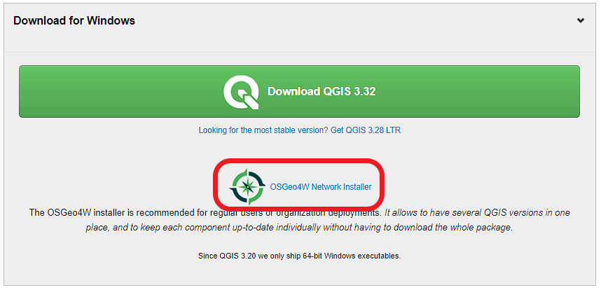 Figure 4.1 Downloading the OSGeo4W installer
 - Click on the link that says "Download OSGeo4W Installer and start it" to downloaded a file called osgeo4w-setup.exe . Then run that file to start the installation.
- Select the "Express Desktop Install" option (Unless you already have OSGeo4W/QGIS installed, then use the Advanced option to ensure you get the latest versions of all packages/tools or pick a different installation folder. If you get errors attempting to run QGIS, you may have to delete your c:\OSGEO4W folder and re-run the installation.)
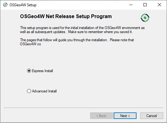 Figure 4.2 Selecting the Express Desktop Install option
 - If asked, select a site from which to install (does not matter which)
- When asked which packages to install, select the options shown in the screenshot below. Apart from that you can accept the default settings on the next pages.
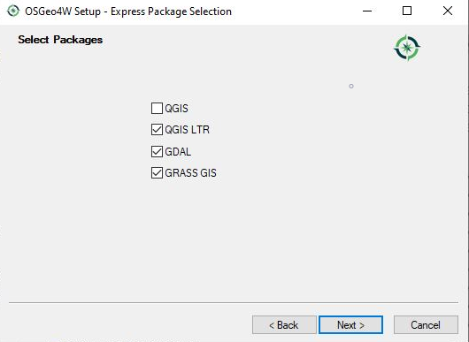 Figure 4.2b Selecting the packages to install
 - Accept the different licenses and run the installation (ignore warnings about corrupted packages if you get them and just click 'Next' if you get warnings about missing dependencies)
Where to find what?
After the installation has finished, you should have a folder called OSGeo4W in the root folder of your C: drive (unless you picked a different folder for the installation). Here we list the main programs from this installation folder that you will need in this lesson:
- C:\OSGeo4W\OSGeo4W.bat - This opens the OSGeo4W shell that can be used for executing python scripts from the command line.
- C:\OSGeo4W\bin\qgis-ltr-bin.exe - This is the main QGIS executable that you need to run for starting QGIS 3.
- C:\OSGeo4W\apps\Qt5\bin\designer.exe - This is the QT Designer executable that you can use for creating Qt5 GUIs in this lesson. If you simply double-click the .exe file in the Windows File Explorer, you will most likely get an DLL related error message because some environment variables won't be set correctly. But you should be able to run the program by opening the OSGeo4W shell and typing the command designer there.
- python-qgis-ltr - As explained further below, you can use this command in the OSGeo4W shell for setting the path and environment variables for running qgis and PyQT5 based Python 3 code as well as executing scripts directly.
Running OSGeo4W shell and commands for qgis and PyQt5 development
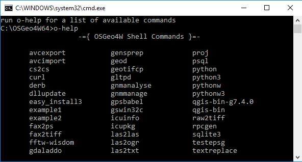
When you run OSGeo4W.bat, the OSGeo4W shell will show up looking similar to the normal Windows command line but providing some additional commands that can be listed by typing in "o-help".
When using the OSGeo4W shell in this lesson, it is best to always execute the command
python-qgis-ltr
first to make sure all environment variables are set up correctly for running qgis and PyQt5 based Python code. The command will start a Python interpreter (recongnizable by the >>> prompt) that you can immediately leave again by typing the command quit() . You can also directly run Python scripts with python-qgis-ltr by writing
python-qgis-ltr xyz.py
rather than just
python xyz.py
You can also use the command pyrcc5 in the OSGeo4W shell for compiling QT5 resource files that we will need later on in this lesson.
Installing geopy package and pandas
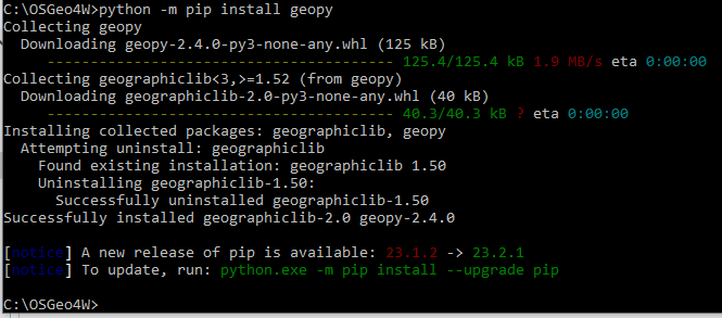
Most of the Python packages we will need in this lesson (like PyQt5) are already installed in the Python environment that comes with OSGeo4W/QGIS, but a few additional pieces are necessary. There is one package that we will use for performing distance calculations between WGS84 points in the two walkthroughs of the lesson. The package is called geopy and it needs to be installed first. To do this, please open the OSGeo4W shell and change to Python 3 by running the python-qgis-ltr command followed by quit() as described above, and then run the following pip installation command:
python -m pip install geopy
The package is small, so the installation should only take a couple of seconds. The output you are getting may look slightly different than what is shown in the image below but should indicate that geopy has been installed successfully.
In the practice exercise for this lesson, we will also use pandas. In earlier versions of QGIS/OSGeo4W, pandas wasn't installed by default. To make sure, simply run the following command for installing pandas; most likely it's going to tell you that pandas is already installed:
python -m pip install pandas
Installing the required QGIS plugins
We will need a few QGIS plugins in this lesson, so let's install those as well. Some of these are for the optional part at the end but they are small and installation should be quick, so let's install all of them now. Please follow the instructions below for this:
- Start QGIS
- Go to Plugins -> Manage and Install Plugins in the main menu bar
- Under "Settings", make sure the box next to "Show also experimental plugins" is checked.
- Under "Not installed" look for the following three plugins and install them:
- QuickMapServices (allows for quickly adding basemaps like OSM to a project)
- Plugin Builder 3 (for creating templates for new plugins)
- Plugin Reloader (for reloading a plugin after modifying the code)
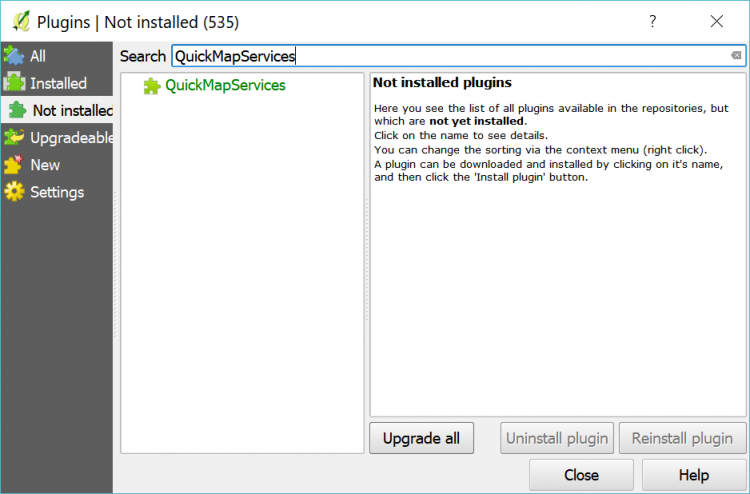
If you now click on "Installed", all three plugins should appear in the list of installed plugins with a checkmark on the left, which indicates that the plugin is activated.
4.4.2 Familiarizing yourself with QGIS
Important note: This lesson has a lot of content and this is one of its less important sections. We included it so that, if you have not worked with QGIS before, you get an idea of where to find what and how things work in QGIS in general. However, since we will mainly be using the QGIS programming API rather than doing things in QGIS itself, we recommend that you go through this section quickly and then maybe come back at the end of the lesson if you have an interest in learning more about QGIS and its interface.
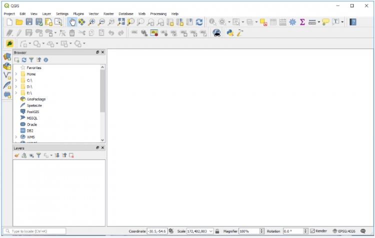
When you open QGIS 3 for the first time, it will look similar to the image below. The main elements are the main menu bar at the top, a number of horizontal toolbars with buttons for different operations below the menu bar, a smaller vertical toolbar on the left side with buttons for adding or creating layers, and then three main windows: a panel with a file browser, a panel that lists the layers in your project (currently empty), and then the main window for displaying the current project. At the very bottom, you can find a status bar displaying information related to the project window such as the scale and coordinate reference system used. Overall, this all looks somewhat similar to ArcGIS Desktop or Pro. All toolbars and panels can be freely moved around, undocked and docked back again, and there are many additional panels and toolbars that can be enabled/disabled either from the main menu under View -> Panels/Toolbars or by doing a right-click on one of the panel title bars or toolbar areas at the top and left.
There are several ways to add a data set to a project:
- By navigating to a file in the file browser panel and then double-clicking it.
- By dragging a file from the Windows File Explorer onto the project window or layers panel.
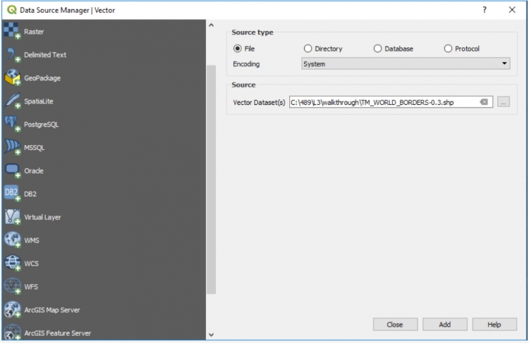
- By clicking the “Open Data Source Manager”
 button, which will open up a dialog with a list of different types of sources on the left including local files, datasets from different databases, and also data sets provided as web services (WMS, WFS, ArcGIS Map Server or Feature Server, etc.).
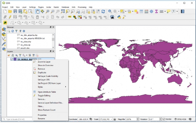
Feel free to try out adding different data sets to the project. Similar to ArcGIS, the coordinate reference system used for the project and project window will be that of the first source added, but of course this can be changed, e.g. by going Project -> Project Properties…. in the menu bar or by left-clicking the CRS field in the status bar. Dragging the layers and the buttons at the top of the Layers panel can be used to arrange the layers in a certain order and group or filter them. We here add the world borders layer from Lesson 3 to the project. The layer now shows up in the project window and the Layers panel. Right-clicking the layer in the Layers panel will provide a number of options for that layer. Double-clicking the layer will directly open the “Layer Properties” dialog with a lot of options to change rendering or other properties of the layer.
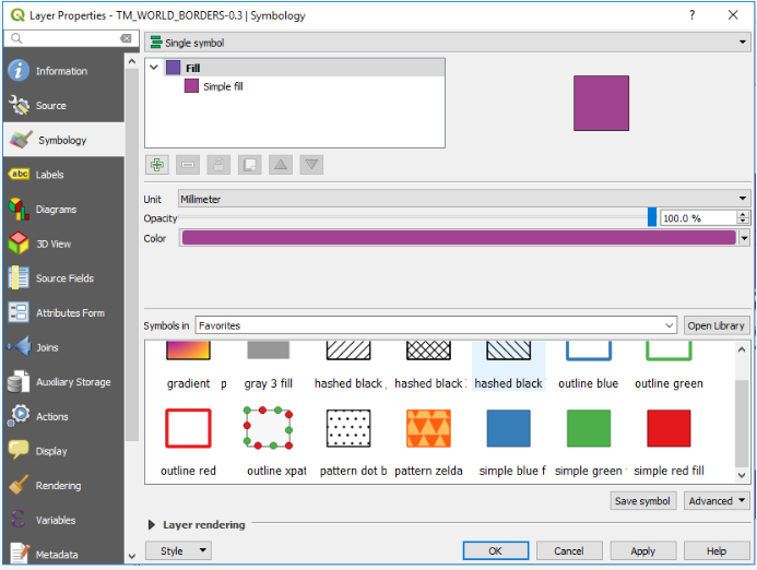
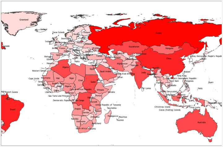
The properties you will most commonly work with are the Symbology and Labels properties. When coming from ArcGIS, working with these dialogs requires a bit of getting used to. Give it a try by attempting to show the world borders layer with a Graduated scheme based on the “AREA” attribute of the layer using a Natural Breaks classification with 8 classes and with labels based on the “NAME” attribute. The result should look somewhat similar to the image below. If you have any problems achieving this, please post on the Lesson 4 discussion forum.
If you want to select features from a layer based on attribute, the Query Builder dialog can be opened by doing a right-click -> Filter … on the layer in the Layers panel. The dialog itself works roughly similar to the corresponding component of ArcGIS. You can check out the attribute table of the layer by doing a right-click -> Open Attribute Table. Working with the attribute table again is roughly similar to ArcGIS. If you want to export a layer as a new data set, you do a right-click -> Export -> Save Features as… . This, for instance, allows for saving only the currently selected features and/or saving the layer in a different format or using a different CRS.
Looking at the main menu bar, we find the main tools for working with Vector and Raster data under the respective submenus. They include typical geoprocessing, data manipulation, and analysis tools. Additional tools can be accessed by opening the Processing Toolbox panel under Processing -> Toolbox. Moreover, QGIS has a plugin interface that allows for writing extensions to QGIS. Plugins can be managed and new plugins can be installed under Plugins -> Manage and Install Plugins, and they can add new entries to menu bar and tool bars. QGIS plugins are written in Python, and you will learn how to do so later on in this lesson. QGIS also has a Python Console (Plugins -> Python Console) that allows for entering and executing Python code that uses the QGIS Python API.
A QGIS project is saved as a .qgz file using Project -> Save or Project -> Save As…. From this menu, you can also open a new project, export the project map in different formats, etc.
One thing that works a bit differently than in ArcGIS is the layout composer component for creating map views of your project including additional elements such as a legend, scale bar, etc. By going Project -> New Print Layout, you can create a new map layout document. This opens up a new window with its own interface that allows you to arrange maps and other elements like images and text in the same way as in a vector graphics or publishing tool. The created layout can just be a single page or span multiple pages and contain different maps. Elements are added to the page with the buttons from the toolbar on the left. A list of all elements is shown in the panel on the top right. The properties of the currently selected element can be accessed and changed with the panel on the bottom right. The simple layout in the image below was created by adding our current map with the add map  button, adding a text element with the add text button
  , and then adding a legend for the current map with the add legend
  button.
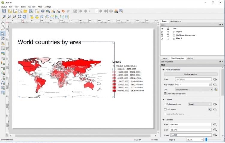
Layouts can be exported as images or PDF files and previously created layouts can be accessed via the Layout Manager under Project -> Layout Manager… or directly be accessed from Project -> Layouts -> … .
This short overview should be enough to get you started but, of course, only covers the basics. This lesson will focus on the QGIS Python API and using it to write programs or plugins for QGIS, rather than on working with the QGIS interface directly. Nevertheless, if you want to learn more about QGIS at some point, the following tutorials covering certain tasks in more detail can be used as a starting point.
- Making a map [3]
- Working with attributes [4]
- Basic vector styling [5]
- Raster styling and analysis [6]
More tutorials are available at this QGIS Tutorials and Tips page [7].