4.5 The QGIS Scripting Interface and Python API
QGIS has a Python programming interface that allows for extending its functionality and for writing scripts that automate QGIS based workflows either inside QGIS or as standalone applications. The Python package that provides this interface is simply called qgis but often referred to as pyQGIS. Its functionality overlaps with what is available in packages that you already know such as arcpy, GDAL/ORG, and the Esri Python API. In the following, we provide a brief introduction to the API so that you are able to perform standard operations like loading and writing vector data, manipulating features and their attributes, and performing selection and geoprocessing operations.
4.5.1 Interacting with Layers Open in QGIS
Let’s start this introduction by writing some code directly in the QGIS Python console and talking about how you can access the layers currently open in QGIS and add new layers to the currently open project. If you don’t have QGIS running at the moment, please start it up and open the Python console from the Plugins menu in the main menu bar.
When you open the Python console in QGIS, the Python qgis package and its submodules are automatically imported as well as other relevant modules including the main PyQt5 modules. In addition, a variable called iface is set up to provide an object of the class QgisInterface1 [1] to interact with the running QGIS environment. The code below shows how you can use that object to retrieve a list of the layers in the currently open map project and the currently active layer. Before you type in and run the code in the console, please add a few layers to an empty project including the TM_WORLD_BORDERS-0.3.shp shapefile that we already used in Section 3.9.1 on GDAL/ORG. We will recreate some of the steps from that section with QGIS here so that you also get a bit of a comparison between the two APIs. The currently active layer is the one selected in the Layers window; please select the world borders layer by clicking on it before you execute the code.
layers = iface.mapCanvas().layers()
for layer in layers:
	print(layer)
	print(layer.name())
	print(layer.id())
	print('------')
# If you copy/paste the code - run the part above
# before you run the part below
# otherwise you'll get a syntax error.
activeLayer = iface.activeLayer()
print('active layer: ' + activeLayer.name())
Output (numbers will vary): ...<qgis._core.QgsVectorLayer object at 0x000000666CF22D38> TM_WORLD_BORDERS-0.3 TM_WORLD_BORDERS_0_3_2e5a7cd5_591a_4d45_a4aa_cbba2e639e75 ------ ... active layer: TM_WORLD_BORDERS-0.3
The layers() method of the QgsMapCanvas [2] object we get from calling iface.mapCanvas() returns the currently open layers as a list of objects of the different subclasses of QgsMapLayer [3]. Invoking the name() method of these layer objects gives us the name under which the layer is listed in the Layers window. layer.id() gives us the ID that QGIS has assigned to the layer which in contrast to the name is unique. The iface.activeLayer() method gives us the currently selected layer.
The type() function of a layer can be used to test the type of the layer:
if activeLayer.type() == QgsMapLayer.VectorLayer:
	print('This is a vector layer!')
Depending on the type of the layer, there are other methods that we can call to get more information about the layer. For instance, for a vector layer [4] we can use wkbType() to get the geometry type of the layer:
if activeLayer.type() == QgsMapLayer.VectorLayer:
	if activeLayer.wkbType() == QgsWkbTypes.MultiPolygon:
		print('This layer contains multi-polygons!')
The output you get from the previous command should confirm that the active world borders layer contains multi-polygons, meaning features that can have multiple polygonal parts.
QGIS defines a function dir(…) that can be used to list the methods that can be invoked for a given object. Try out the following two applications of this function:
dir(iface)
dir(activeLayer)
To add or remove a layer, we need to work with the QgsProject [5] object for the project currently open in QGIS. We retrieve it like this:
currentProject = QgsProject.instance()
print(currentProject.fileName())
The output from the print statement in the second row will probably be the empty string unless you have saved the project. Feel free to do so and rerun the line and you should get the actual file name.
Here is how we can remove the active layer (or any other layer object) from the layer registry of the project (you may have to resize/refresh the map canvas afterwards for the layer to disappear there):
currentProject.removeMapLayer(activeLayer.id())
The following command shows how we can add the world borders shapefile again (or any other feature class we have on disk). Make sure you adapt the path based on where you have the shapefile stored. We first have to create the vector layer object providing the file name and optionally the name to be used for the layer. Then we add that layer object to the project via the addMapLayer(…) method:
layer = QgsVectorLayer(r'C:\489\TM_WORLD_BORDERS-0.3.shp', 'World borders')
currentProject.addMapLayer(layer)
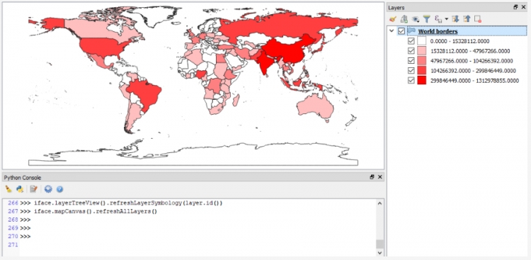
Lastly, here is an example that shows you how you can change the symbology of a layer from your code:
renderer = QgsGraduatedSymbolRenderer()
renderer.setClassAttribute('POP2005')
layer.setRenderer(renderer)
layer.renderer().updateClasses(layer, QgsGraduatedSymbolRenderer.Jenks, 5)
layer.renderer().updateColorRamp(QgsGradientColorRamp(Qt.white, Qt.red))
iface.layerTreeView().refreshLayerSymbology(layer.id())
iface.mapCanvas().refreshAllLayers()
Here we create an object of the QgsGraduatedSymbolRenderer class that we want to use to draw the country polygons from our layer using a graduated color approach based on the population attribute ‘POP2005’. The name of the field to use is set via the renderer’s setClassAttribute() method in line 2. Then we make the renderer object the renderer for our world borders layer in line 3. In the next two lines, we tell the renderer (now accessed via the layer method renderer()) to use a Jenks Natural Breaks classification with 5 classes and a gradient color ramp that interpolates between the colors white and red. Please note that the colors used as parameters here are predefined instances of the Qt5 class QColor. Changing the symbology does not automatically refresh the map canvas or layer list. Therefore, in the last two lines, we explicitly tell the running QGIS environment to refresh the symbology of the world borders layer in the Layers tree view (line 6) and to refresh the map canvas (line 7). The result should look similar to the figure below (with all other layers removed).
You will get to see another example of interacting with the layers open in QGIS and setting the symbology (for point and line layers in this case) in Section 4.12 where we take the code from this lesson's walkthrough and turn it into a QGIS plugin.
[1] The qgis Python module is a wrapper around the underlying C++ library. The documentation pages linked in this section are those of the C++ version but the names of classes and available functions and methods are the same.
4.5.2 Accessing the Features of a Layer
Let’s keep working with the world borders layer open in QGIS for a bit, looking at how we can access the individual features in a layer and select features by attribute. The following piece of code shows you how we can loop through all the features with the help of the layer’s getFeatures() method:
for feature in layer.getFeatures():
    print(feature)
    print(feature.id())
    print(feature['NAME'])
    print('-----')
Output:
<qgis._core.QgsFeature object at 0x...>
0
Antigua and Barbuda
-----
<qgis._core.QgsFeature object at 0x...>
1
Algeria
-----
<qgis._core.QgsFeature object at 0x...>
2
Azerbaijan
-----
<qgis._core.QgsFeature object at 0x...>
3
Albania
-----
...
Features are represented as objects of the class QgsFeature [6] in QGIS. So, for each iteration of the for-loop in the previous code example, variable feature will contain a QgsFeature object. Features are numbered with a unique ID that you can obtain by calling the method id() as we are doing in this example. Attributes like the NAME attribute of the world borders polygons can be accessed using the attribute name as the key as also demonstrated above.
Like in most GIS software, a layer can have an active selection. When the layer is open in QGIS, the selected features are highlighted. The layer method selectAll() allows for selecting all features in a layer and removeSelection() can be used to clear the selection. Give this a try by running the following two commands in the QGIS Python console and watch how all countries become selected and then deselected again.
layer.selectAll()
layer.removeSelection()
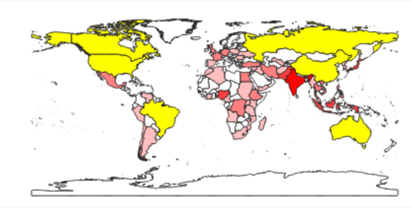
The method selectByExpression() allows for selecting features based on their properties with a SQL query string that has the same format as in ArcGIS. Use the following command to select all features from the layer that have a value larger than 300,000 in the AREA column of the attribute table. The result should look as in the figure below.
layer.selectByExpression('"AREA" > 300000')
While there can only be one active selection for a layer, you can create as many subgroups of features from a layer as you want by calling getFeatures(…) with a parameter that is an object of the class QgsFeatureRequest [7] and that has been given a filter expression via its setFilterExpression(…) method. The filter expression can be again an SQL query string. The following code creates a subgroup that will only contain the polygon for Canada. When you run it, this will not change the active selection that you see for that layer in QGIS but variable selectionName now provides access to the subgroup with just that one polygon. We get that first (and only) polygon by calling the __next__() method of selectionName and then print out some information about this particular polygon feature.
selectionName = layer.getFeatures(QgsFeatureRequest().setFilterExpression('"NAME" = \'Canada\''))
feature = selectionName.__next__()
print(feature['NAME'] + "-" + str(feature.id()))
print(feature.geometry())
print(feature.geometry().asWkt())
Output:
Canada – 23
<qgis._core.QgsGeometry object at 0x...>
MultiPolygon (((-65.61361699999997654 43.42027300000000878,...)))
The first print statement in this example works in the same way as you have seen before to get the name attribute and id of the feature. The method geometry() gives us the geometric object for this feature as an instance of the QgsGeometry class [8] and calling the method asWkt() gives us a WKT string representation of the multi-polygon geometry. You can also use a for-loop to iterate through the features in a subgroup created in this way. The method rewind() can be used to reset the iterator to the beginning so that when you call __next__() again, it will again give you the first feature from the subgroup.
When you have the geometry object and know what type of geometry it is, you can use the methods asPoint(), asPolygon(), asPolyline(), asMultiPolygon(), etc. to get the geometry as a Python data structure, e.g. in the case of multi-polygons as a list of lists of lists with each inner list containing tuples of the point coordinates for one polygonal component.
print(feature.geometry().asMultiPolygon())
[[[(-65.6136, 43.4203), (-65.6197,43.4181), … ]]]
Here is another example to demonstrate that we can work with several different subgroups of features at the same time. This time we request all features from the layer that have a POP2005 value larger than 50,000,000.
selectionPopulation = layer.getFeatures(QgsFeatureRequest().setFilterExpression('"POP2005" > 50000000'))
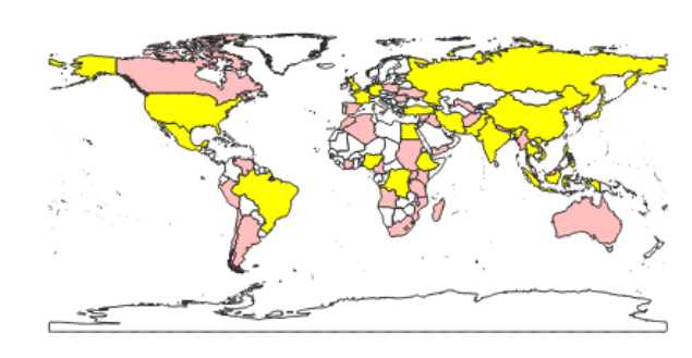
If we ever want to use a subgroup like this to create the active selection for the layer from it, we can use the layer method selectByIds(…) for this. The method requires a list of feature IDs and will then change the active selection to these features. In the following example, we use a simple list comprehension to create the ID list from the subgroup in our variable selectionPopulation:
layer.selectByIds([f.id() for f in selectionPopulation])
When running this command you should notice that the selection of the features in QGIS changes to look like in the figure below.
Let’s save the currently selected features as a new file. We use the GeoPackage format (GPKG) for this, which is more modern than the shapefile format, but you can easily change the command below to produce a shapefile instead; simply change the file extension to “.shp” and replace “GPKG” with “ESRI Shapefile”. The function we will use for writing the layer to disk is called writeAsVectorFormat(…) and it is defined in the class QgsVectorFileWriter [9]. Please note that this function has been declared "deprecated", meaning it may be removed in future versions and it is recommended that you do not use it anymore. In versions up to QGIS 3.16 (the current LTR version that most likely you are using right now), you are supposed to use writeAsVectorFormatV2(...) instead; however, there have been issues reported with that function and it is already replaced by writeAsVectorFormatV3(...) in versions >3.16 of QGIS. Therefore, we have decided to stick with writeAsVectorFormat(…) while things are still in flux. The parameters we give to writeAsVectorFormat(…) are the layer we want to save, the name of the output file, the character encoding to use, the spatial reference to use (we simply use the one that our layer is in), the format (“GPKG”), and True for signaling that only the selected features should be saved in the new data set. Adapt the path for the output file as you see fit and then run the command:
QgsVectorFileWriter.writeAsVectorFormat(layer, r'C:\489\highPopulationCountries.gpkg', 'utf-8', layer.crs(),'GPKG', True)
If you add the new file produced by this command to your QGIS project, it should only contain the polygons for the countries we selected based on their population values.
For changing the attribute values of a feature, we need to work with the “data provider” object of the layer. We can access it via the layer’s dataProvider() method:
dataProvider = layer.dataProvider()
Let’s say we want to change the POP2005 value for Canada to 1 (don’t ask what happened!). For this, we also need the index of the POP2005 column which we can get by calling the data provider’s fieldNameIndex() method:
populationColumnIndex = dataProvider.fieldNameIndex('POP2005')
To change the attribute value we call the method changeAttributeValues(…) of the data provider object providing a dictionary as parameter that maps feature IDs to dictionaries which in turn map column indices to new values. The inner dictionary that maps column indices to values is defined in a separate variable newValueDictionary.
newValueDictionary = { populationColumnIndex : 1 }
dataProvider.changeAttributeValues( { feature.id(): newValueDictionary } )
In this simple example, the outer dictionary contains only a single key-value pair with the ID of the feature for Canada as key and another dictionary as value. The inner dictionary also only contains a single key-value pair consisting of the index of the population column and its new value 1. Both dictionaries can have multiple entries to simultaneously change multiple values of multiple features. After running this command, check out the attributes of Canada, either via the QGIS Identify tool or in the attribute table of the layer. You will see that the population value in the layer now has been changed to 1 (the same holds for the underlying shapefile). Let’s set the value back to what it was with the following command:
dataProvider.changeAttributeValues( { feature.id(): { populationColumnIndex : 32270507 } } )
4.5.3 Creating Features and Geometric Operations
For the final part of this section, let’s switch from the Python console in QGIS to writing a standalone script that uses qgis. You can use your editor of choice to write the script and then execute the .py file from the OSGeo4W shell (see again Section 4.4.1) with all environment variables set correctly for a qgis and QT5 based program.
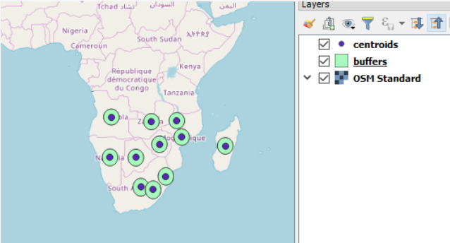
We are going to repeat the task from Section 3.9.1 of creating buffers around the centroids of the countries within a rectangular (in terms of WGS 84 coordinates) area around southern Africa. We will produce two new vector GeoPackage files: a point based one with the centroids and a polygon based one for the buffers. Both data sets will only contain the country name as their only attribute.
We start by importing the modules we will need and creating a QApplication() (handled by qgis.core.QgsApplication) for our program that qgis can run in (even though the program does not involve any GUI).
Important note: When you later write you own qgis programs (e.g. in the L4 homework assignment), make sure that you always "import qgis" first before using any other qgis related import statements such as "import qgis.core". We are not sure why this is needed, but the other imports will most likely fail tend to fail without "import qgis" coming first.
import os, sys
import qgis
import qgis.core
To use qgis in our software, we have to initialize it and we need to tell it where the actual QGIS installation is located. To do this, we use the function getenv(…) of the os module to get the value of the environmental variable “QGIS_PREFIX_PATH” which will be correctly defined when we run the program from the OSGeo4W shell. Then we create an instance of the QgsApplication class and call its initQgis() method.
qgis_prefix = os.getenv("QGIS_PREFIX_PATH")
qgis.core.QgsApplication.setPrefixPath(qgis_prefix, True)
qgs = qgis.core.QgsApplication([], False)
qgs.initQgis()
Now we can implement the main functionality of our program. First, we load the world borders shapefile into a layer (you may have to adapt the path!).
layer = qgis.core.QgsVectorLayer(r'C:\489\TM_WORLD_BORDERS-0.3.shp')
Then we create the two new layers for the centroids and buffers. These layers will be created as new in-memory layers and later written to GeoPackage files. We provide three parameters to QgsVectorLayer(…): (1) a string that specifies the geometry type, coordinate system, and fields for the new layer; (2) a name for the layer; and (3) the string “memory” which tells the function that it should create a new layer in memory from scratch (rather than reading a data set from somewhere else as we did earlier).
centroidLayer = qgis.core.QgsVectorLayer("Point?crs=" + layer.crs().authid() + "&field=NAME:string(255)", "temporary_points", "memory")
bufferLayer = qgis.core.QgsVectorLayer("Polygon?crs=" + layer.crs().authid() + "&field=NAME:string(255)", "temporary_buffers", "memory")
The strings produced for the first parameters will look like this: “Point?crs=EPSG:4326&field=NAME:string(255)” and “Polygon?crs=EPSG:4326&field=NAME:string(255)”. Note how we are getting the EPSG string from the world border layer so that the new layers use the same coordinate system, and how an attribute field is described using the syntax “field=<name of the field>:<type of the field>". When you want your layer to have more fields, these have to be separated by additional & symbols like in a URL.
Next, we set up variables for the data providers of both layers that we will need to create new features for them. The new features will be collected in two lists, centroidFeatures and bufferFeatures.
centroidProvider = centroidLayer.dataProvider()
bufferProvider = bufferLayer.dataProvider()

centroidFeatures = []
bufferFeatures = []
Then, we create the polygon geometry for our selection area from a WKT string as in Section 3.9.1:
areaPolygon = qgis.core.QgsGeometry.fromWkt('POLYGON ( (6.3 -14, 52 -14, 52 -40, 6.3 -40, 6.3 -14) )')
In the main loop of our program, we go through all the features in the world borders layer, use the geometry method intersects(…) to test whether the country polygon intersects with the area polygon, and, if yes, create the centroid and buffer features for the two layers from the input feature.
for feature in layer.getFeatures():
    if feature.geometry().intersects(areaPolygon):
        centroid = qgis.core.QgsFeature()
        centroid.setAttributes([feature['NAME']])
        centroid.setGeometry(feature.geometry().centroid())
        centroidFeatures.append(centroid)

        buffer = qgis.core.QgsFeature()
        buffer.setAttributes([feature['NAME']])
        buffer.setGeometry(feature.geometry().centroid().buffer(2.0,100))
        bufferFeatures.append(buffer)
Note how in both cases (centroids and buffers), we first create a new QgsFeature object, then use setAttributes(…) to set the NAME attribute to the name of the country, and then use setGeometry(…) to set the geometry of the new feature either to the centroid derived by calling the centroid() method or to the buffered centroid created by calling the buffer(…) method of the centroid point. As a last step, the new features are added to the respective lists. Finally, all features in the two lists are added to the layers after the for-loop has been completed. This happens with the following two commands:
centroidProvider.addFeatures(centroidFeatures)
bufferProvider.addFeatures(bufferFeatures)
Lastly, we write the content of the two in-memory layers to GeoPackage files on disk. This works in the same way as in previous examples. Again, you might want to adapt the output paths.
qgis.core.QgsVectorFileWriter.writeAsVectorFormat(centroidLayer, r'C:\489\centroids.gpkg', "utf-8", layer.crs(), "GPKG")
qgis.core.QgsVectorFileWriter.writeAsVectorFormat(bufferLayer, r'C:\489\buffers.gpkg', "utf-8", layer.crs(), "GPKG")
Since we are now done with using QGIS functionalities (and actually the entire program), we clean up by calling the exitQgis() method of the QgsApplication, freeing up resources that we don’t need anymore.
qgs.exitQgis()
If you run the program from the OSGeo4W shell and then open the two produced output files in QGIS, the result should look as shown in the image below.
4.5.4 (Geo)processing
QGIS has a toolbox system and visual workflow building component somewhat similar to ArcGIS and its Model Builder. It is called the QGIS processing framework [10]and comes in the form of a plugin called Processing that is installed by default. You can access it via the Processing menu in the main menu bar. All algorithms from the processing framework are available in Python via a QGIS module called processing. They can be combined to solve larger analysis tasks in Python and can also be used in combination with the other qgis methods discussed in the previous sections.
We can get a list of all processing algorithms currently registered with QGIS with the command QgsApplication.processingRegistry().algorithms(). Each processing object in the returned list has an identifying name that you can get via its id() method. The following command, which you can try out in the QGIS Python console, uses this approach to print the names of all algorithms that contain the word “clip”:
[x.id() for x in QgsApplication.processingRegistry().algorithms() if "clip" in x.id()]
Output:

['gdal:cliprasterbyextent', 'gdal:cliprasterbymasklayer','gdal:clipvectorbyextent', 'gdal:clipvectorbypolygon', 'native:clip', 'saga:clippointswithpolygons', 'saga:cliprasterwithpolygon', 'saga:polygonclipping']
As you can see, there are processing versions of algorithms coming from different sources, e.g. natively built into QGIS vs. algorithms based on GDAL. The function algorithmHelp(…) allows you to get some documentation on an algorithm and its parameters. Try it out with the following command:
processing.algorithmHelp("native:clip")
To run a processing algorithm, you have to use the run(…) function and provide two parameters: the id of the algorithm and a dictionary that contains the parameters for the algorithm as key-value pairs. run(…) returns a dictionary with all output parameters of the algorithm. The following example illustrates how processing algorithms can be used to solve the task of clipping a points of interest shapefile to the area of El Salvador, reusing the two data sets from homework assignment 2 (Section 2.10). This example is intended to be run as a standalone program again and most of the code is required to set up the QGIS environment needed, including initializing the Processing environment.
The start of the script looks like in the example from the previous section:
import os,sys
import qgis
import qgis.core

qgis_prefix = os.getenv("QGIS_PREFIX_PATH")
qgis.core.QgsApplication.setPrefixPath(qgis_prefix, True)
qgs = qgis.core.QgsApplication([], False)
qgs.initQgis()
After, creating the QGIS environment, we can now initialize the processing framework. To be able to import the processing module we have to make sure that the plugins folder is part of the system path; we do this directly from our code. After importing processing, we have to initialize the Processing environment and we also add the native QGIS algorithms to the processing algorithm registry.
# Be sure to change the path to point to where your plugins folder is located
# it may not be the same as this one.
sys.path.append(r"C:\OSGeo4W\apps\qgis-ltr\python\plugins")
import processing
from processing.core.Processing import Processing
Processing.initialize()
qgis.core.QgsApplication.processingRegistry().addProvider(qgis.analysis.QgsNativeAlgorithms())
Next, we create input variables for all files involved, including the output files we will produce, one with the selected country and one with only the POIs in that country. We also set up input variables for the name of the country and the field that contains the country names.
poiFile = r'C:\489\L2\assignment\OSMpoints.shp'
countryFile = r'C:\489\L2\assignment\countries.shp'
pointOutputFile = r'C:\489\L2\assignment\pointsInCountry.shp'
countryOutputFile = r'C:\489\L2\assignment\singleCountry.shp'

nameField = "NAME"
countryName = "El Salvador"
Now comes the part in which we actually run algorithms from the processing framework. First, we use the qgis:extractbyattribute algorithm to create a new shapefile with only those features from the country data set that satisfy a particular attribute query. In the dictionary with the input parameters for the algorithm, we specify the name of the input file (“INPUT”), the name of the query field (“FIELD”), the comparison operator for the query (0 here stands for “equal”), and the value to which we are comparing (“VALUE”). Since the output will be written to a new shapefile, we don’t really need the output dictionary that we get back from calling run(…) but the print statement shows how this dictionary in this case contains the name of the output file under the key “OUTPUT”.
output = processing.run("qgis:extractbyattribute", { "INPUT": countryFile, "FIELD": nameField, "OPERATOR": 0, "VALUE": countryName, "OUTPUT": countryOutputFile  })
print(output['OUTPUT'])
To perform the clip operation with the new shapefile from the previous step, we use the “native:clip” algorithm. The input paramters are the input file (“INPUT”), the clip file (“OVERLAY”), and the output file (“OUTPUT”). Again, we are just printing out the content stored under the “OUTPUT” key in the returned dictionary. Finally, we exit the QGIS environment.
output = processing.run("native:clip", { "INPUT": poiFile, "OVERLAY": countryOutputFile, "OUTPUT": pointOutputFile })
print(output['OUTPUT'])

qgs.exitQgis()
Below is how the resulting two layers should look when shown in QGIS in combination with the original country layer.
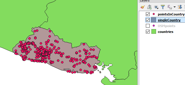
In this section, we showed you how to perform common GIS operations with the QGIS Python API. Once again we have to say that we are only scratching the surface here; the API is much more complex and powerful, and there is hardly anything you cannot do with it. What we have shown you will be sufficient to understand the code from the two walkthroughs of this lesson, but, if you want more, below are some links to further examples. Keep in mind though that since QGIS 3 is not that old yet, some of the examples on the web have been written for QGIS 2.x. While many things still work in the same way in QGIS 3, you may run into situations in which an example won’t work and needs to be adapted to be compatible with QGIS 3.